Solidification of small para-H₂ clusters at zero temperature

Abstract

We have determined the ground-state energies of para-H₂ clusters at zero temperature using the diffusion Monte Carlo method. The liquid or solid character of each cluster is investigated by restricting the phase through the use of proper importance sampling. Our results show inhomogeneous crystallization of clusters, with alternating behavior between liquid and solid phases up to $N=55$. From there on, all clusters are solid. The ground-state energies in the range $N=13$–75 are established and the stable phase of each cluster is determined. In spite of the small differences observed between the energy of liquid and solid clusters, the corresponding density profiles are significantly different, feature that can help to solve ambiguities in the determination of the specific phase of H₂ clusters.

I Introduction

Molecular para-hydrogen has been suggested from long time ago as the possible second natural superfluid after liquid ⁴He. ginzburg However, the H₂-H₂ interaction is so deeply attractive that it crystallizes before arriving to the superfluid transition temperature. The advantage of having half the mass of ⁴He is therefore not enough to compensate the hydrogen strong attraction and para-H₂ becomes solid at temperature $T=13.96$ K. Many attempts to supercool liquid hydrogen down to the expected lambda transition ($T_{\lambda}=1-2$ K) have been unfruitful, at least for the bulk phase.clark Partial success has only been achieved in confined geometries, mainly in small pure liquid drops tejeda or bigger drops in a ⁴He environment. vilesov

Para-H₂ clusters have been the object of many studies in the last years ceperley1 ; guardiola1 ; cuervo ; bonin1 due to the primary interest of determining i) its liquid or solid character and ii) the dependence of superfluidity on the size and temperature of the cluster. The first path integral Monte Carlo (PIMC) simulation of H₂ clusters, carried out by Sindzingre et al., ceperley1 showed that clusters comprising up to a number of molecules $N\simeq 18$ are superfluid at temperatures below $T=2$ K. The maximum number of molecules that shows superfluid behavior has been enlarged up to $N\simeq 26$ in a recent PIMC simulation where lower temperatures $T=0.5$ K have been analyzed. ceperley2 The results obtained in Ref. ceperley2 show evidence of superfluidity mostly localized in the surface of the cluster, pointing to an inhomogeneous structure with an inner solid core surrounded by a liquid skin that, at the lowest temperatures, is superfluid. This localized superfluidity has been questioned in a recent PIMC calculation where it has been shown that superfluidity is a global property of the cluster in spite of its significant spatial structure. bonin2 In the limit of zero temperature, the structure and energy of small H₂ clusters have been accurately studied using both diffusion Monte Carlo (DMC) guardiola1 ; guardiola2 and path integral ground state (PIGS). cuervo Both at finite and zero temperature the simulations show the presence of magic-cluster sizes in which the chemical potential shows a kink. These more stable $N$ configurations have also been observed experimentally in cryogenic free jet expansions using Raman spectroscopy. tejeda

In the present work, we address the question of the solidification of para-H₂ clusters in the limit of zero temperature and as a function of the number of molecules. Our aim is the screening of the more stable ground-state structure by performing simulations where the phase (liquid or solid) is kept fixed. To this end, we use the diffusion Monte Carlo (DMC) method that solves stochastically the $N$-body Schrödinger equation exactly for bosons, within some statistical errors. Differently from previous studies using DMC, we have focused our attention on the discrimination between liquid and solid phases as a function of the number of molecules. This goal is achieved by carrying out parallel simulations for liquid and solid configurations at each $N$, with special effort on the search for optimal lattices on which to build trial wave functions for the solid clusters. With the present study, we show which is the energetically preferred phase at $T=0$ for each $N$, in the range $13\leq N\leq 75$, and how the energy difference between the two type of clusters changes with increasing $N$.

The rest of the paper is organized as follows. In the next Section, we present our theoretical approach that relies on the DMC method. In Sec. III, we report our results on the energetic and structure properties of the para-H₂ clusters in the $N$ range analyzed. Finally, we end with the summary and main conclusions in Sec. IV.

II Quantum Monte Carlo approach

Our study of para-H₂ clusters relies on a purely microscopic approach whose inputs are only the interparticle interaction and the mass. Our goal is the study of these finite systems at zero temperature to deal with their ground state. To this end, we use the DMC method which is able to generate exact (within statistical uncertainty) information through guided random walks. The starting point in the DMC method is the $N$-body Schrödinger equation, written in imaginary time

$$-\frac{\partial\Psi({\bf R},t)}{\partial t}=(H-E)\,\Psi({\bf R},t)\ ,$$ (1)

with ${\bf R}\equiv({\bf r}_{1},\ldots,{\bf r}_{N})$, a $3N$-dimensional vector (walker), and $t$ the imaginary time measured in units of $\hbar$. The time-dependent wave function of the system $\Psi({\bf R},t)$ can be expanded in terms of a complete set of eigenfunctions $\phi_{i}({\bf R})$ of the Hamiltonian,

$$\Psi({\bf R},t)=\sum_{n}c_{n}\,\exp\left[\,-(E_{i}-E)t\,\right]\,\phi_{i}({\bf R})\ ,$$ (2)

where $E_{i}$ is the eigenvalue associated to $\phi_{i}({\bf R})$. Consequently, the asymptotic solution of 1, for any value $E$ close to the energy of the ground state and for long times ($t\rightarrow\infty$), gives $\phi_{0}({\bf R})$, provided that there is a nonzero overlap between $\Psi({\bf R},t=0)$ and the ground-state wave function $\phi_{0}({\bf R})$.

A direct Monte Carlo implementation of 1 is hardly able to work efficiently, especially when the interatomic potential contains a hard core. This is solved by using importance sampling. The importance sampling technique is a general concept in Monte Carlo and is one of the best methods to reduce the variance of any MC calculation. The importance sampling method, applied to 1, consists in rewriting the Schrödinger equation in terms of the wave function

$$f({\bf R},t)\equiv\psi({\bf R})\,\Psi({\bf R},t)\ ,$$ (3)

$\psi({\bf R})$ being a time-independent variational wave function that describes approximately the ground state of the system. Considering a Hamiltonian of the form

$$H=-\frac{\hbar^{2}}{2\,m}\,{\mbox{\boldmath$\nabla$}}^{2}_{{\bf R}}+V({\bf R})\ ,$$ (4)

1 turns out to be

$$-\frac{\partial f({\bf R},t)}{\partial t}=-D\,{\mbox{\boldmath$\nabla$}}^{2}_{{\bf R}}f({\bf R},t)+D\,{\mbox{\boldmath$\nabla$}}_{{\bf R}}\left({\bf F}({\bf R})\,f({\bf R},t)\,\right)+\left(E_{L}({\bf R})-E\right)\,f({\bf R},t)\ ,$$ (5)

where $D=\hbar^{2}/(2m)$, $E_{L}({\bf R})=\psi({\bf R})^{-1}H\psi({\bf R})$ is the local energy, and

$${\bf F}({\bf R})=2\,\psi({\bf R})^{-1}{\mbox{\boldmath$\nabla$}}_{{\bf R}}\psi({\bf R})$$ (6)

is called drift or quantum force. ${\bf F}({\bf R})$ acts as an external force which guides the diffusion process, involved by the first term in 5, to regions where $\psi({\bf R})$ is large.

The r.h.s. of 5 may be written as the action of three operators $A_{i}$ acting on the wave function $f({\bf R},t)$,

$$-\frac{\partial f({\bf R},t)}{\partial t}=(A_{1}+A_{2}+A_{3})\,f({\bf R},t)\equiv A\,f({\bf R},t)$$ (7)

The three terms $A_{i}$ may be interpreted by similarity with classical differential equations. The first one, $A_{1}$, corresponds to a free diffusion with a a diffusion coefficient $D$; $A_{2}$ acts as a driving force due to an external potential, and finally $A_{3}$ looks like a birth/death term. In Monte Carlo, the Schrödinger equation 7 is best suited when it is written in an integral form by introducing the Green function $G({\bf R}^{\prime},{\bf R},t)$, which gives the transition probability from an initial state ${\bf R}$ to a final one ${\bf R}^{\prime}$ during a time $t$,

$$f({\bf R}^{\prime},t+\Delta t)=\int G({\bf R}^{\prime},{\bf R},\Delta t)\,f({\bf R},t)\,d{\bf R}\ .$$ (8)

More explicitly, the Green function is given in terms of the operator $A=A_{1}+A_{2}+A_{3}$ by

$$G({\bf R}^{\prime},{\bf R},\Delta t)=\left\langle\,{\bf R}^{\prime}\,|\,\exp(-A\Delta t)\,|\,{\bf R}\,\right\rangle.$$ (9)

DMC algorithms rely on reasonable approximations of $G({\bf R}^{\prime},{\bf R},\Delta t)$ for small values of the time-step $\Delta t$. We work with a second-order expansion of the exponential [9] to reduce the time-step dependence. boronat Once a short-time approximation is assumed, 9 is iterated repeatedly until reaching the asymptotic regime $f({\bf R},t\rightarrow\infty)$, a limit in which one is effectively sampling the ground state.

Para-H₂ is a boson particle with total spin 0 and with rotational ground-state state $J=0$. It is well described by a merely radial interaction due to its high-degree sphericity. Among the different interatomic potentials proposed for describing the H₂-H₂ intermolecular interaction, we have chosen the Silvera-Goldman potential silvera due to its proved accuracy and its dominant use in microscopic calculations as the present one. The well depth of the molecular hydrogen interaction is $\sim-37$ K, a factor of four larger than in helium, making the ground-state phase of bulk at zero temperature be an hcp crystal in spite of H₂ mass being half the ⁴He one.

The trial wave function used for importance sampling is written as the product of one- and two-body correlation factors,

$$\psi({\bf R})=\prod_{1=i<j}^{N}e^{u(r_{ij})}\,\prod_{i=1}^{N}e^{v(r_{iI})}\ ,$$ (10)

with

$$u(r) = -\frac{1}{2}\left(\frac{b}{r}\right)^{5}-\frac{\beta r}{N}$$ (11)

$$v(r) = -\alpha r^{2}\ .$$ (12)

The two-body term $u(r)$ accounts for the correlations induced by the potential $V(r)$ and also for the finite size of the system that implies the wave function approaches zero when the distance is of the order of the cluster size. The one-body term $v(r)$ is only used for solid clusters and localizes particles around the preferred sites (capital indexes in 10). This model wave function for the solid, with the one-body Gaussian terms, is the well-know Nosanow-Jastrow (NJ) wave function that has been widely used in the study of bulk quantum solids. The NJ wave function is not symmetric under the exchange of particles but the influence in the energy of symmetrization is known to be of the order of miliKelvin bernu and therefore indistinguishable within our statistical errors. Recently, it has been proposed a symmetrized NJ wave function to study superfluidity in bulk solid ⁴He and proved that the change in energy due to Bose symmetry on top of the NJ model is imperceptible, within the numerical resolution of quantum Monte Carlo. cazorla It is worth noticing that the effect of symmetrization in the structure of para-H₂ clusters at temperature $T=1.5$ K has been recently studied by Warnecke et al.; warnecke the results obtained show a very small influence of Bose statistics on the density profiles, the energy differences being not reported.

The parameters entering in Eq. (11) and Eq. (12) have been optimized using the variational Monte Carlo (VMC) method. For liquid configurations the optimal parameters are: $b=3.58$ Å, $\beta=2.79$ Å^-1, and $\alpha=0$; for solid ones: $b=3.32$ Å, $\beta=0$, and $\alpha=0.521$ Å^-2. These are the VMC optimal parameters for $N=40$ but the dependence of these parameters with $N$ is tiny: for $N=13$, $\beta=2.30$ Å^-1, $\alpha=0.360$ Å^-2, and $b$ is the same. In DMC we have neglected this slight $N$ dependence because the results are insensitive to it. On the other hand, two technical issues related to the implementation of the DMC method, i.e., the time-step dependence and the number of walkers, have been accurately analyzed to reduce any systematic bias to the level of the statistical noise.

The simulation of solid clusters with the NJ wave function we are using requires of a set of lattice points. In the case of bulk solids, the number of possible lattices is few, well known and easy to characterize geometrically. When dealing with finite systems, the issue of the best geometrical arrangement is somehow universal for the smallest structures, where Mackay polyhedra are the preferred structures, but it becomes more complex when the number of particle increases. Moreover, the determination of the optimal solid patterns are normally obtained using classical physics and the influence on those of quantum delocalization is less known. Our strategy for this optimization has been the use of both simulated annealing (SA) and ab initio random search (method for finding structures where the total classical force felt by any particle is approximately zero). The structures of minimum energy predicted for both approaches essentially coincide for $N\leq 30$, but for larger $N$ values the SA method has proven to be better. In the SA approach, we have used both an exponential annealing schedule and another with constant thermodynamic speed. McKeown The search for any $N$ has been carried out by starting from 20–40 random configurations and selecting the best ones for a posterior quantum simulation. In some cases, we have performed additional optimizations using long classical Monte Carlo simulations. Finally, we used the best classical solutions as initial setup for the quantum simulations and reported in all cases the lowest energy achieved. It is worth mentioning that we introduced a scaling factor $f_{\rm s}$ in the quantum simulation,

$${\bf r}_{i}^{\rm s}=({\bf r}_{i}-{\bf r}_{\rm CM})f_{\rm s}\ ,$$ (13)

with ${\bf r}_{\rm CM}$ the center of mass of the cluster and ${\bf r}_{i}$ ($i=1,\ldots,N$) the SA points, to allow for possible spatial expansions or contractions of the classic lattice points but the optimal energy was always the corresponding to the classic solutions ($f_{\rm s}=1$).

III Results

We have calculated the energy and structure properties of H₂ clusters in the range $13\leq N\leq 75$ using the DMC method discussed in the preceding Section. At each $N$, we have used both the liquid and solid trial wave functions introduced in Sec. II. In 1, we show the results for the energy per particle obtained for both phases and for clusters up to $N=55$ molecules. The difference between both configurations is small in all the $N$ range studied pointing to a highly correlated liquid, even for the lightest clusters. The energy per particle in absolute value increases with $N$ for both phases but solid clusters have energies with a kind of zigzag dependence whereas the liquid ones follow a smoother law. The irregular behavior of the energy of solid clusters is consequence of the appearance of magic numbers, with geometrically more compact structures that make them more stable.

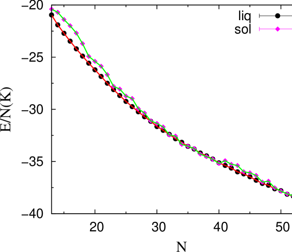
Figure 1: (Color online) Energy per particle of H₂ clusters as a function of $N$. Circles and diamonds stand for liquid and solid phases, respectively. The lines are guides to the eye. Error bars are smaller than the size of the symbols

The difference between the energies of liquid and solid clusters is shown explicitly in 2. Starting from $N=13$, the energy of liquid clusters is clearly preferred but the difference $(E_{L}-E_{S})/N$ decreases when $N$ increases. According to our results, the first cluster that is solid in its ground state is the one with $N=32$. From $N=33$ to 40, there are some solid clusters but for $N=41$ and the following ones there is again a liquid regime. Arriving to $N=55$, one enters definitively in a preferred solid phase that persists up to $N=75$ which is the largest cluster here analyzed. The more intriguing aspect of our results is the existence of a liquid stability island for $N=41$–50 between the initial solid regime and the second one, that we think is the stable one for $N>55$. It can be argued that the nonuniform crystallization of H₂ clusters that we have observed can be due to our model of solid clusters. We can not discard completely this argument but we have performed a rather exhaustive search of lattice points, as commented in the preceding Section, and the results remain unchanged.

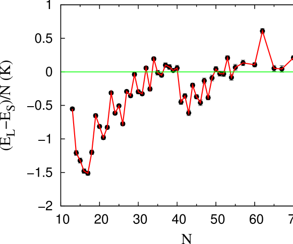
Figure 2: (Color online) Difference between the energies per particle of liquid and solid clusters ($(E_{L}-E_{S})/N$) as a function of $N$.

An important part of our simulation has been the search of optimal structures for solid clusters. The most useful tool has been the simulated annealing algorithm that, in spite of being completely classical, has proven to be able to generate the best configurations. A simple check for that has been the optimization of a scaling parameter $f_{\rm s}$ that we introduced to make possible contractions or expansions of the classical solution. Systematically, the optimal solution has been $f_{\rm s}=1$. In 3, the best lattice points for solid clusters with $N=18$, 19, and 20 are shown. We have joined with lines the planar structures to get a better visualization of the clusters. The case $N=19$ corresponds to a well-know magic number and it is in fact a structure that we identify in a lot of clusters. As one can see in 3, in the clusters $N=18$ and $N=20$ the one-defect and one-excess structures, with respect to the geometrically perfect $N=19$ lattice, are clearly observed.

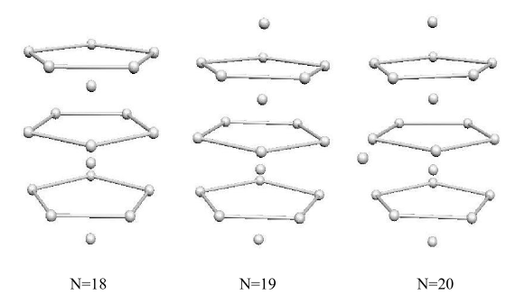
Figure 3: (Color online) Optimal distribution of lattice points for solid clusters with $N=18$, 19, and 20.

The effort of achieving optimal structures increases significantly with $N$, so a lot of SA simulations with different initial configurations have been carried out. Our best configurations coincide with reported ones for Lennard-Jones interactions up to $N\simeq 30$. web For larger $N$ values, our results differ significantly from the published ones web and we get systematically better energies with our structures. In 4, we report our optimal lattice points for clusters with $N=31$ and $N=34$, i.e., beyond the regime where our predictions are compatible with the ones from Ref. web . As commented before, it is quite remarkable that the inner structure of these two clusters is the same and coincides exactly with the magic structure of $N=19$. Around this well-defined structure it starts to appear a second pentagonal shell which is only complete in the center and concentric with the central pentagon of the $N=19$ cluster.

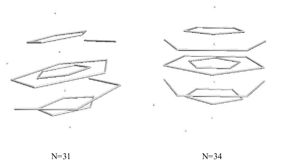
Figure 4: (Color online) Optimal distribution of lattice points for solid clusters with $N=31$ and 34.

In Table 1, we report the ground-state energies for each $N$ and the corresponding phase. Our results for the liquid clusters agree with the previous results of Ref. guardiola2 obtained also using the DMC method and the same interaction potential. The present results for the solid clusters are new and never calculated before. The energies reported in Table 1 lead to persistence of liquid character up to relatively large $N$ values, in particular to larger values than the ones reported in previous PIMC estimations at finite temperature. ceperley2 ; bonin2 Nevertheless, the difference in energy between the two phases remains small even for the largest clusters studied. We made several attempts at simulating clusters with an inner solid core and a liquid surface but we were not able to get any improvement of the energy with respect to the optimal values reported in the table.

Table 1: Energy per particle of the ground state of para-H₂ clusters as a function of $\bf{N}$. The phase of the cluster is labeled L and S for liquid and solid, respectively. Figures in parenthesis are the statistical errors.

$N$	$E/N$ (K)	Phase	$N$	$E/N$ (K)	Phase
13	$-20.952(16)$	L	38	$-34.531(16)$	S
14	$-21.904(14)$	L	39	$-34.785(17)$	S
15	$-22.709(11)$	L	40	$-35.184(17)$	S
16	$-23.466(12)$	L	41	$-35.376(27)$	L
17	$-24.199(16)$	L	42	$-35.630(27)$	L
18	$-24.901(17)$	L	43	$-35.993(35)$	L
19	$-25.576(17)$	L	44	$-36.184(25)$	L
20	$-26.215(14)$	L	45	$-36.459(27)$	L
21	$-26.847(16)$	L	46	$-36.796(38)$	L
22	$-27.500(18)$	L	47	$-37.099(31)$	L
23	$-28.111(12)$	L	48	$-37.278(28)$	L
24	$-28.671(18)$	L	49	$-37.615(38)$	L
25	$-29.237(19)$	L	50	$-37.837(24)$	S
26	$-29.737(17)$	L	51	$-38.131(32)$	L
27	$-30.235(14)$	L	52	$-38.326(33)$	L
28	$-30.710(22)$	L	53	$-38.726(11)$	S
29	$-31.141(22)$	L	54	$-38.787(39)$	L
30	$-31.646(24)$	L	55	$-38.942(23)$	S
31	$-32.013(22)$	L	57	$-39.382(24)$	S
32	$-32.454(15)$	S	60	$-39.820(19)$	S
33	$-32.818(26)$	L	62	$-40.629(19)$	S
34	$-33.357(15)$	S	65	$-40.543(19)$	S
35	$-33.547(27)$	L	67	$-40.882(19)$	S
36	$-33.804(19)$	L	70	$-41.409(17)$	S
37	$-34.287(18)$	S	75	$-41.711(24)$	S

Figure 5: (Color online) Chemical potential of H₂ clusters as a function of $N$.

The possibility of magic clusters, with higher probability of being experimentally observed due to its enhanced stability, has deserved the attention of all the theoretical and experimental works in this subject. If such structures exist, one can see its signature in energy differences, mainly in the chemical potential defined as

$$\mu(N)=E(N)-E(N-1)\ .$$ (14)

In 5, we show the results for the chemical potential [14] obtained from the DMC ground-state energies reported in Table 1. In the liquid regime (small clusters), $\mu(N)$ is quite a smooth function with small local minima for $N=23$, 25, and 30. For $N>30$, a clear zigzag structure is observed with some minima that correspond to liquid clusters and other that are solid. Therefore, the chemical potential we obtain is no more a smooth function as derived in previous DMC estimations where only liquid clusters where considered. guardiola1 ; guardiola2 Our results show a more complex structure with some alternating phases and with a lot of local minima, mainly when entering in the solid phase.

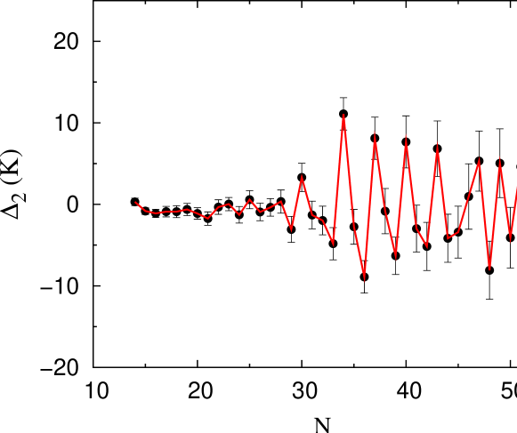
Figure 6: (Color online) Second energy difference $\Delta_{2}$ of H₂ clusters as a function of $N$.

The issue of the existence of magic clusters can be better analyzed by calculating the second energy difference,

$$\Delta_{2}(N)=E(N+1)-2E(N)+E(N-1)\ .$$ (15)

DMC results for $\Delta_{2}(N)$ are shown in Fig. 6. The observed pattern emphasizes the behavior of $\mu(N)$, with a quite smooth behavior up to $N\sim 30$ and sharp peaks beyond this value. By looking at the position of the maxima, we observe magic structures for $N=13$, 19, 23, 25, 28, 30, 34, 37, 40, 43, 47, 49, 51, and 53. Some of these values have been recently found in PIMC simulations at finite temperatures. navarro ; mezzacapo

DMC simulations serve also to calculate structure properties of the clusters, as for instance, the density profiles. In 7, we show the density profiles of clusters with $N=19$ and $N=29$ using both the liquid and solid trial wave functions. As one can see, the size of the cluster is very similar for liquid and solid clusters with the same $N$ but the inner structure is rather different. This is particularly clear for $N=19$ where the central density of the liquid is large whereas for the solid is zero. This central zero density for the solid cluster can be well understood by inspection of the lattice points of the $N=19$ cluster reported in 3. When $N$ increases, the differences between liquid and solid clusters diminish but are still clear for the case $N=29$ reported in 7. It is worth noticing that the density profiles of the liquid clusters present a two-shell effect guardiola1 ; cuervo ; ceperley1 ; bonin1 due to the strong intermolecular H₂-H₂ attraction that is never observed in liquid ⁴He clusters.

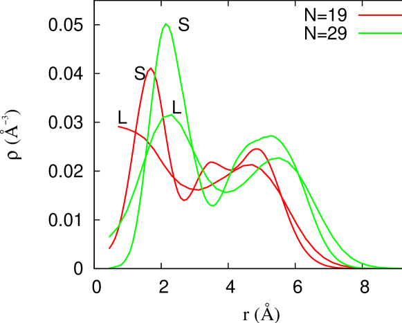
Figure 7: (Color online) Density profiles of H₂ clusters with $N=19$ and 29. Labels L and S stand for liquid and solid clusters, respectively.

Figure 8: Density profiles of liquid H₂ clusters with $N=19$, 21, 23, 25, 27, and 29. The line for each $N$ can be identified looking at the radius of the cluster that increases monotonically with $N$.

We report the evolution of the density profiles of liquid and solid clusters with $N$ in 8 and 9, respectively. Increasing $N$ in the liquid clusters produces a continuous change in the density profile: the central density decreases to zero and a two-shell structure, that moves progressively to larger $r$, clearly appears. In the case of solid clusters (9), the evolution with $N$ is not so smooth, mainly for the lowest $N$ values. Different from the liquid clusters, solid ones show always empty density in the center of the cluster and additional structure between the two shells that tend to dissappear when $N$ becomes larger. Comparing density profiles for the same $N$ and different phase, one concludes that functions $\rho(r)$ are in all cases different enough to be unambiguously discerned in spite of the fact that the difference between their binding energies is less that 1 K per particle.

Figure 9: Density profiles of solid H₂ clusters with $N=19$, 21, 23, 25, 27, and 29. The line for each $N$ is of the same type than in Fig. 7.

IV Conclusions

H₂ clusters in the range $N=13$–75 have been microscopically characterized at zero temperature using the DMC method. Controlling the phase of the cluster by using different models for trial wave functions used for importance sampling we have been able to determine the ground-state stable phase for each $N$ in the range analyzed. Our results point to a nonuniform crystallization of the H₂ clusters, with some alternating behavior between the two phases depending on the particular $N$ value. For clusters with $N\geq 55$ the stable phase is the solid one. The structure of the clusters, as shown in their density profiles, is significantly different for liquid and solid clusters with the same $N$, even when the difference in energy between both is really tiny. Therefore, the shape of the density profiles can help to identify the nature of these clusters both in experiment and in finite-temperature simulations.

References

- (1) Ginzburg, V.L.; Sobyanin, A.A. JETP Lett. 1972, 15, 242.
- (2) Clark, A.C.; Lin X.; Chan, M.H. W. Phys. Rev. Lett. 2006, 97, 245301.
- (3) Tejeda, G.; Fernández, J.M.; Montero, S.; Blume, D.; Toennies, J.P. Phys. Rev. Lett. 2004, 92, 223401.
- (4) Kuyanov-Prozumnet, K.; Vilesov, A.F. Phys. Rev. Lett. 2008, 101, 205301.
- (5) Sindzingre, P.; Ceperley, D.M.; Klein, M.L. Phys. Rev. Lett. 1991, 67, 1871.
- (6) Guardiola, R.; Navarro, J. Phys. Rev. A 2006, 74, 025201.
- (7) Cuervo, J.E.; Roy, P.N. J. Chem. Phys. 2006, 125, 124314.
- (8) Mezzacapo, F.; Boninsegni, M. Phys. Rev. Lett. 2006, 97, 045301.
- (9) Khairallah, S.A.; Sevryuk, M.B.; Ceperley, D. M.; Toennies, J.P. Phys. Rev. Lett. 2007, 98, 183401.
- (10) Mezzacapo, F.; Boninsegni, M. Phys. Rev. Lett. 2008, 100, 145301.
- (11) Guardiola, R.; Navarro, J. Cent. Eur. J. Phys. 2008, 6, 33.
- (12) Boronat, J.; Casulleras, J. Phys. Rev. B 1994, 49, 8920.
- (13) Silvera, I.F.; Goldman, V.V. J. Chem. Phys. 1978, 69, 4209.
- (14) Ceperley, D.M.; Bernu, B. Phys. Rev. Lett. 2004, 93, 155303.
- (15) Cazorla, C.; Astrakharchik, G.E.; Casulleras, J.; Boronat, J. New J. Phys. 2009, 11, 013407.
- (16) Warnecke S.; Sevryuk, M.B.; Ceperley D.M.; Toennies, J.P.; Guardiola, R.; Navarro, J. Eur. Phys. J. D 2010, 56, 353.
- (17) MacKeown, P. K. Stochastic Simulation in Physics, Springer-Verlag: Singapore, 1997.
- (18) http://www-doye.ch.cam.ac.uk/jon/structures/LJ/tables.150.html
- (19) Navarro, J.; Guardiola, R. Int. J. Quant. Chem. 2011, 111, 463.
- (20) Mezzacapo, F.; Boninsegni, M. J. Phys.: Condens. Matter 2009, 21, 164205.