Multiple Kernel Learning: A Unifying Probabilistic Viewpoint

Abstract

We present a probabilistic viewpoint to multiple kernel learning unifying well-known regularised risk approaches and recent advances in approximate Bayesian inference relaxations. The framework proposes a general objective function suitable for regression, robust regression and classification that is lower bound of the marginal likelihood and contains many regularised risk approaches as special cases. Furthermore, we derive an efficient and provably convergent optimisation algorithm.

Keywords: Multiple kernel learning, approximate Bayesian inference, double loop algorithms, Gaussian processes

1 Introduction

Nonparametric kernel methods, cornerstones of machine learning today, can be seen from different angles: as regularised risk minimisation in function spaces (Schölkopf and Smola, 2002), or as probabilistic Gaussian process methods (Rasmussen and Williams, 2006). In these techniques, the kernel (or equivalently covariance) function encodes interpolation characteristics from observed to unseen points, and two basic statistical problems have to be mastered. First, a latent function must be predicted which fits data well, yet is as smooth as possible given the fixed kernel. Second, the kernel function parameters have to be learned as well, to best support predictions which are of primary interest. While the first problem is simpler and has been addressed much more frequently so far, the central role of learning the covariance function is well acknowledged, and a substantial number of methods for “learning the kernel”, “multiple kernel learning”, or “evidence maximisation” are available now. However, much of this work has firmly been associated with one of the “camps” (referred to as regularised risk and probabilistic in the sequel) with surprisingly little crosstalk or acknowledgments of prior work across this boundary. In this paper, we clarify the relationship between major regularised risk and probabilistic kernel learning techniques precisely, pointing out advantages and pitfalls of either, as well as algorithmic similarities leading to novel powerful algorithms.

We develop a common analytical and algorithmical framework encompassing approaches from both camps and provide clear insights into the optimisation structure. Even though, most of the optimisation is non convex, we show how to operate a provably convergent “almost Newton” method nevertheless. Each step is not much more expensive than a gradient based approach. Also, we do not require any foreign optimisation code to be available. Our framework unifies kernel learning for regression, robust regression and classification.

The paper is structured as follows: In section 2, we introduce the regularised risk and the probabilistic view of kernel learning. In increasing order of generality, we explain multiple kernel learning (MKL, section 2.1), maximum a posteriori estimation (MAP, section 2.2) and marginal likelihood maximisation (MLM, section 2.3). A taxonomy of the mutual relations between the approaches and important special cases is given in section 2.4. Section 3 introduces a general optimisation scheme and section 4 draws a conclusion.

2 Kernel Methods and Kernel Learning

Kernel-based algorithms come in many shapes, however, the primary goal is – based on training data $\{(\mathbf{x}_{i},y_{i})\,|\,i=1..n\}$, $\mathbf{x}_{i}\in{\cal X}$, $y_{i}\in\mathcal{Y}$ and a parametrised kernel function $k_{\bm{\theta}}(\mathbf{x},\mathbf{x}^{\prime})$ – to predict the output $y_{*}$ for unseen inputs $\mathbf{x}_{*}$. Often, linear parametrisations $k_{\bm{\theta}}(\mathbf{x},\mathbf{x}^{\prime})=\sum_{m=1}^{M}\theta_{m}k_{m}(\mathbf{x},\mathbf{x}^{\prime})$ are used, where the $k_{m}$ are fixed positive definite functions, and $\bm{\theta}\succeq\mathbf{0}$. Learning the kernel means finding $\bm{\theta}$ to best support this goal. In general, kernel methods employ a postulated latent function $u:{\cal X}\to\mathbb{R}$ whose smoothness is controlled via the function space squared norm $\|u(\cdot)\|_{k_{\bm{\theta}}}^{2}$. Most often, smoothness is traded against data fit, either enforced by a loss function $\ell(y_{i},u(\mathbf{x}_{i}))$ or modeled by a likelihood $\mathbb{P}(y_{i}|u_{i})$. Let us define kernel matrices $\mathbf{K}_{\bm{\theta}}:=[k_{\bm{\theta}}(\mathbf{x}_{i},\mathbf{x}_{j})]_{ij}$, and $\mathbf{K}_{m}:=[k_{m}(\mathbf{x}_{i},\mathbf{x}_{j})]_{ij}$ in $\mathbb{R}^{n\times n}$ and the vectors $\mathbf{y}:=[y_{i}]_{i}\in\mathcal{Y}^{n}$, $\mathbf{u}:=[u(\mathbf{x}_{i})]_{i}\in\mathbb{R}^{n}$ collecting outputs and latent function values, respectively.

The regularised risk route to kernel prediction, which is followed by any support vector machine (SVM) or ridge regression technique, yields $\|u(\cdot)\|_{k_{\bm{\theta}}}^{2}+\frac{C}{n}\sum_{i=1}^{n}\ell(y_{i},u_{i})$ as criterion, enforcing smoothness of $u(\cdot)$ as well as good data fit through the loss function $\frac{C}{n}\ell(y_{i},u(\mathbf{x}_{i}))$. By the representer theorem, the minimiser can be written as $u(\cdot)=\sum_{i}\alpha_{i}k_{\bm{\theta}}(\cdot,\mathbf{x}_{i})$, so that $\|u(\cdot)\|_{k_{\bm{\theta}}}^{2}=\bm{\alpha}^{\top}\mathbf{K}_{\bm{\theta}}\bm{\alpha}$ (Schölkopf and Smola, 2002). As $\mathbf{u}=\mathbf{K}_{\bm{\theta}}\bm{\alpha}$, the regularised risk problem is given by

$$\min_{\mathbf{u}}\mathbf{u}^{\top}\mathbf{K}_{\bm{\theta}}^{-1}\mathbf{u}+\frac{C}{n}\sum_{i=1}^{n}\ell(y_{i},u_{i}).$$ (1)

A probabilistic viewpoint of the same setting is based on the notion of a Gaussian process (GP) (Rasmussen and Williams, 2006): a Gaussian random function $u(\cdot)$ with mean function $\mathbb{E}[u(\mathbf{x})]=m(\mathbf{x})\equiv 0$ and covariance function $\mathbb{V}[u(\mathbf{x}),u(\mathbf{x}^{\prime})]=\mathbb{E}[u(\mathbf{x})u(\mathbf{x}^{\prime})]=k_{\bm{\theta}}(\mathbf{x},\mathbf{x}^{\prime})$. In practice, we only use finite-dimensional snapshots of the process $u(\cdot)$: for example, $\mathbb{P}(\mathbf{u};\bm{\theta})=\mathcal{N}(\mathbf{u}|\mathbf{0},\mathbf{K}_{\bm{\theta}})$, a zero-mean joint Gaussian with covariance matrix $\mathbf{K}_{\bm{\theta}}$. We adopt this GP as prior distribution over $u(\cdot)$, estimating the latent function as maximum of the posterior process $\mathbb{P}(u(\cdot)|\mathbf{y};\bm{\theta})\propto\mathbb{P}(\mathbf{y}|\mathbf{u})\mathbb{P}(u(\cdot);\bm{\theta})$. Since the likelihood depends on $u(\cdot)$ only through the finite subset $\{u(\mathbf{x}_{i})\}$, the posterior process has a finite-dimensional representation: $\mathbb{P}(u(\cdot)|\mathbf{y},\mathbf{u})=\mathbb{P}(u(\cdot)|\mathbf{u})$, so that $\mathbb{P}(u(\cdot)|\mathbf{y};\bm{\theta})=\int\mathbb{P}(u(\cdot)|\mathbf{u})\mathbb{P}(\mathbf{u}|\mathbf{y};\bm{\theta})\text{d}\mathbf{u}$ is specified by the joint distribution $\mathbb{P}(\mathbf{u}|\mathbf{y};\bm{\theta})$, a probabilistic equivalent of the representer theorem. Kernel prediction amounts to maximum a posteriori (MAP) estimation

$$\max\nolimits_{\mathbf{u}}\mathbb{P}(\mathbf{u}|\mathbf{y};\bm{\theta})\equiv\max\nolimits_{\mathbf{u}}\mathbb{P}(\mathbf{u};\bm{\theta})\mathbb{P}(\mathbf{y}|\mathbf{u})\equiv\min\nolimits_{\mathbf{u}}\mathbf{u}^{\top}\mathbf{K}_{\bm{\theta}}^{-1}\mathbf{u}-2\ln\mathbb{P}(\mathbf{y}|\mathbf{u})+\ln|\mathbf{K}_{\bm{\theta}}|,$$ (2)

ignoring an additive constant. Minimising equations (1) and (2) for any fixed kernel matrix $\mathbf{K}$ gives the same minimiser $\hat{\mathbf{u}}$ and prediction $u(\mathbf{x}_{*})=\hat{\mathbf{u}}^{\top}\mathbf{K}_{\bm{\theta}}^{-1}[k_{\bm{\theta}}(\mathbf{x}_{i},\mathbf{x}_{*})]_{i}$.

The correspondence between likelihood and loss function bridges probabilistic and regularised risk techniques. More specifically, any likelihood $\mathbb{P}(\mathbf{y}|\mathbf{u})$ induces a loss function $\ell(\mathbf{y},\mathbf{u})$ via

$$-2\ln\mathbb{P}(\mathbf{y}|\mathbf{u})=-2\sum_{i}\ln\mathbb{P}(y_{i}|u_{i})\rightsquigarrow\frac{C}{n}\sum_{i=1}^{n}\ell(y_{i},u_{i})=\ell(\mathbf{y},\mathbf{u}),$$

however some loss functions cannot be interpreted as a negative log likelihood as shown in table (2) and as discussed for the SVM by Sollich (2000). If, the likelihood is a log-concave function of $\mathbf{u}$, it corresponds to a convex loss function (Boyd and Vandenberghe, 2002, Sect. 3.5.1). Common loss functions and likelihoods for classification $\mathcal{Y}=\{\pm 1\}$ and regression $\mathcal{Y}=\mathbb{R}$ are listed in table (2).

$\mathcal{Y}$	Loss function	$\ell(y_{i},u_{i})$	$\mathbb{P}(y_{i}|u_{i})$	Likelihood
$\{\pm 1\}$	SVM Hinge loss	$\max(0,1-y_{i}u_{i})$	$\nexists$
$\{\pm 1\}$	Log loss	$\ln(\exp(-y_{i}u_{i})+1)$	$1/(\exp(-\tau y_{i}u_{i})+1)$	Logistic
$\mathbb{R}$	SVM $\epsilon$-insensitive loss	$\max(0,|y_{i}-u_{i}|/\epsilon-1)$	$\nexists$
$\mathbb{R}$	Quadratic loss	$(y_{i}-u_{i})^{2}$	$\mathcal{N}(y_{i}|u_{i},\sigma^{2})$	Gaussian
$\mathbb{R}$	Linear loss	$|y_{i}-u_{i}|$	$\mathcal{L}(y_{i}|u_{i},\tau)$	Laplace

Table 1: Relations between loss functions and likelihoods

In the following, we discuss several approaches to learn the kernel parameters $\bm{\theta}$ and show how all of them can be understood as instances of or approximations to Bayesian evidence maximisation. Although the exposition MKL section 2.1 and MAP section 2.2 use a linear parametrisation $\bm{\theta}\mapsto\mathbf{K}_{\bm{\theta}}=\sum_{m=1}^{M}\theta_{m}\mathbf{K}_{m}$, much of the results in MLM 2.3 and all the aforementioned discussion are still applicable to non-linear parametrisations.

2.1 Multiple Kernel Learning

A widely adopted regularised risk principle, known as multiple kernel learning (MKL) (Christianini et al., 2001; Lanckriet et al., 2004; Bach et al., 2004), is to minimise equation (1) w.r.t. the kernel parameters $\bm{\theta}$ as well. One obvious caveat is that for any fixed $\mathbf{u}$, equation (1) becomes ever smaller as $\theta_{m}\to\infty$: it cannot per se play a meaningful statistical role. In order to prevent this, researchers constrain the domain of $\bm{\theta}\in\bm{\Theta}$ and obtain

$$\min_{\bm{\theta}\in\bm{\Theta}}\min_{\mathbf{u}}\mathbf{u}^{\top}\mathbf{K}_{\bm{\theta}}^{-1}\mathbf{u}+\ell(\mathbf{y},\mathbf{u}),$$

where $\bm{\Theta}=\{\bm{\theta}\succeq\mathbf{0},\>\|\bm{\theta}\|_{2}\leq 1\}$ or $\bm{\Theta}=\{\bm{\theta}\succeq\mathbf{0},\>\mathbf{1}^{\top}\bm{\theta}\leq 1\}$ (Varma and Ray, 2007). Notably, these constraints are imposed independently of the statistical problem, the model and of the parametrization $\bm{\theta}\mapsto\mathbf{K}_{\bm{\theta}}$. The Lagrangian form of the MKL problem with parameter $\lambda$ and a general $p$-norm unit ball constraint where $p\geq 1$ (Kloft et al., 2009) is given by

$$\min_{\bm{\theta}\succeq\mathbf{0}}\phi_{\text{MKL}}(\bm{\theta}),\;\text{ where }\phi_{\text{MKL}}(\bm{\theta}):=\min_{\mathbf{u}}\mathbf{u}^{\top}\mathbf{K}_{\bm{\theta}}^{-1}\mathbf{u}+\ell(\mathbf{y},\mathbf{u})+\underbrace{\lambda\cdot\mathbf{1}^{\top}\bm{\theta}^{p}}_{\rho(\bm{\theta})},\;\lambda>0.$$ (3)

Since, the regulariser $\rho(\bm{\theta})$ for the kernel parameter $\bm{\theta}$ is convex, the map $(\mathbf{u},\mathbf{K})\mapsto\mathbf{u}^{\top}\mathbf{K}^{-1}\mathbf{u}$ is jointly convex for $\mathbf{K}\succeq\mathbf{0}$ (Boyd and Vandenberghe, 2002) and the parametrisation $\bm{\theta}\mapsto\mathbf{K}_{\bm{\theta}}$ is linear, MKL is a jointly convex problem for $\bm{\theta}\succeq\mathbf{0}$ whenever the loss function $\ell(\mathbf{y},\mathbf{u})$ is convex. Furthermore, there are efficient algorithms to solve equation (3) for large models (Sonnenburg et al., 2006).

2.2 Joint MAP Estimation

Adopting a probabilistic MAP viewpoint, we can minimise equation (2) w.r.t. $\mathbf{u}$ and $\bm{\theta}\succeq\mathbf{0}$:

$$\min_{\bm{\theta}\succeq\mathbf{0}}\phi_{\text{MAP}}(\bm{\theta}),\;\text{ where }\phi_{\text{MAP}}(\bm{\theta}):=\min_{\mathbf{u}}\mathbf{u}^{\top}\mathbf{K}_{\bm{\theta}}^{-1}\mathbf{u}-2\ln\mathbb{P}(\mathbf{y}|\mathbf{u})+\ln|\mathbf{K}_{\bm{\theta}}|.$$ (4)

While equation (3) and equation (4) share the “inner solution” $\hat{\mathbf{u}}$ for fixed $\mathbf{K}_{\bm{\theta}}$ – in case the loss $\ell(\mathbf{y},\mathbf{u})$ corresponds to a likelihood $\mathbb{P}(\mathbf{y}|\mathbf{u})$ – they are different when it comes to optimising $\bm{\theta}$. The joint MAP problem is not in general jointly convex in $(\bm{\theta},\mathbf{u})$, since $\bm{\theta}\mapsto\ln|\mathbf{K}_{\bm{\theta}}|$ is concave, see figure 2. However, it is always a well-posed statistical procedure, since $\ln|\mathbf{K}_{\bm{\theta}}|\to\infty$ as $\theta_{m}\to\infty$ for all $m$.

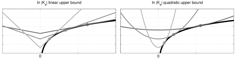
Figure 1: Convex upper bounds on (the concave non-decreasing) $\ln|\mathbf{K}_{\bm{\theta}}|$

By Fenchel duality, we can represent any concave non-decreasing function and hence the log determinant function by $\ln|\mathbf{K}_{\bm{\theta}}|=\min_{\bm{\lambda}\succeq\mathbf{0}}\bm{\lambda}^{\top}|\bm{\theta}|^{p}-g^{*}(\bm{\lambda})$. As a consequence, we obtain a piecewise polynomial upper bound for any particular value $\bm{\lambda}$.

We show in the following, how the regularisers $\rho(\bm{\theta})=\lambda\left\|\bm{\theta}\right\|_{p}^{p}$ of equation (3) can be related to the probabilistic term $f(\bm{\theta})=\ln|\mathbf{K}_{\bm{\theta}}|$. In fact, the same reasoning can be applied to any concave non-decreasing function.

Since the function $\bm{\theta}\mapsto f(\bm{\theta})=\ln|\mathbf{K}_{\bm{\theta}}|$, $\bm{\theta}\succeq\mathbf{0}$ is jointly concave, we can represent it by $f(\bm{\theta})=\min_{\bm{\lambda}\succeq\mathbf{0}}\bm{\lambda}^{\top}\bm{\theta}-f^{*}(\bm{\lambda})$ where $f^{*}(\bm{\lambda})$ denotes Fenchel dual of $f(\bm{\theta})$. Furthermore, the mapping $\bm{\vartheta}\mapsto\ln|\sum_{m=1}^{M}\sqrt[p]{\vartheta_{m}}\mathbf{K}_{m}|=f(\sqrt[p]{\bm{\vartheta}})=g(\bm{\vartheta})$, $\bm{\vartheta}\succeq\mathbf{0}$ is jointly concave due to the composition rule (Boyd and Vandenberghe, 2002, §3.2.4), because $\bm{\vartheta}\mapsto\sqrt[p]{\bm{\vartheta}}$ is jointly concave and $\bm{\theta}\mapsto f(\bm{\theta})$ is non-decreasing in all components $\theta_{m}$ as all matrices $\mathbf{K}_{m}$ are positive (semi-)definite which guarantees that the eigenvalues of $\mathbf{K}_{\bm{\theta}}$ increase as $\theta_{m}$ increases. Thus we can – similarly to Zhang (2010) – represent $\ln|\mathbf{K}_{\bm{\theta}}|$ as

$$\ln|\mathbf{K}_{\bm{\theta}}|=f(\bm{\theta})=g(\bm{\vartheta})=\min_{\bm{\lambda}\succeq\mathbf{0}}\bm{\lambda}^{\top}\bm{\vartheta}-g^{*}(\bm{\lambda})=\min_{\bm{\lambda}\succeq\mathbf{0}}\bm{\lambda}^{\top}|\bm{\theta}|^{p}-g^{*}(\bm{\lambda}).$$

Choosing a particular value $\bm{\lambda}=\lambda\cdot\mathbf{1}$, we obtain the bound $\ln|\mathbf{K}_{\bm{\theta}}|\leq\lambda\cdot\left\|\bm{\theta}\right\|_{p}^{p}-g^{*}(\lambda\cdot\mathbf{1})$. Figure 1 illustrates the bounds for $p=1$ and $p=2$. The bottom line is that one can interpret the regularisers $\rho(\bm{\theta})=\lambda\left\|\bm{\theta}\right\|_{p}^{p}$ in equation (3) as corresponding to parametrised upper bounds to the $\ln|\mathbf{K}_{\bm{\theta}}|$ part in equation (4), hence $\phi_{\text{MKL}}(\bm{\theta})=\psi_{\text{MAP}}(\bm{\theta},\bm{\lambda}=\lambda\cdot\mathbf{1})$, where $\phi_{\text{MAP}}(\bm{\theta})=\min_{\bm{\lambda}\succeq\mathbf{0}}\psi_{\text{MAP}}(\bm{\theta},\bm{\lambda})$. Far from an ad hoc choice to keep $\bm{\theta}$ small, the $\ln|\mathbf{K}_{\bm{\theta}}|$ term embodies the Occam’s razor concept behind MAP estimation: overly large $\bm{\theta}$ are ruled out, since their explanation of the data $\mathbf{y}$ is extremely unlikely under the prior $\mathbb{P}(\mathbf{u};\bm{\theta})$. The Occam’s razor effect depends crucially on the proper normalization of the prior (MacKay, 1992). For example, the weighting parameter $C$ of $k$ ($k=C\tilde{k}$) can be learned by joint MAP: if $C=e^{c}$, then equation (4) is convex in $c$ for any fixed $\mathbf{u}$. If kernel-regularised estimation equation (1) is interpreted as MAP estimation under a GP prior equation (2), the correct extension to kernel learning is joint MAP: the MKL criterion equation (3) lacks prior normalization, which renders MAP w.r.t. $\bm{\theta}$ meaningful in the first place. From a non-probabilistic viewpoint, the $\ln|\mathbf{K}_{\bm{\theta}}|$ term comes with a model and data dependent structure at least as complex as the rest of equation (3).

While the MKL objective, equation (3), enjoys the benefit of being convex in the (linear) kernel parameters $\bm{\theta}$, this does not hold true for joint MAP estimation, equation (4), in general. We illustrate the differences in figure 2. The function $\psi_{\text{MAP}}(\bm{\theta},\mathbf{u})$ is a building block of the MAP objective $\phi_{\text{MAP}}(\bm{\theta})=\min_{\mathbf{u}}[\psi_{\text{MAP}}(\bm{\theta},\mathbf{u})-2\ln\mathbb{P}(\mathbf{y}|\mathbf{u})]$, where

$$\psi_{\text{MAP}}(\bm{\theta},\mathbf{u})=\underbrace{\mathbf{u}^{\top}\mathbf{K}_{\bm{\theta}}^{-1}\mathbf{u}}_{\psi_{\cup}(\bm{\theta},\mathbf{u})}+\underbrace{\ln|\mathbf{K}_{\bm{\theta}}|}_{\psi_{\cap}(\bm{\theta})}\leq\psi_{\text{MKL}}(\bm{\theta},\mathbf{u})-g^{*}(\lambda\cdot\mathbf{1}),\>\psi_{\text{MKL}}(\bm{\theta},\mathbf{u})=\mathbf{u}^{\top}\mathbf{K}_{\bm{\theta}}^{-1}\mathbf{u}+\lambda\left\|\bm{\theta}\right\|_{p}^{p}.$$

More concretely, $\psi_{\text{MAP}}(\bm{\theta},\mathbf{u})$ is a sum of a nonnegative, jointly convex function $\psi_{\cup}(\bm{\theta},\mathbf{u})$ that is strictly decreasing in every component $\theta_{m}$ and a concave function $\psi_{\cap}(\bm{\theta})$ that is strictly increasing in every component $\theta_{m}$. Both functions $\psi_{\cup}(\bm{\theta},\mathbf{u})$ and $\psi_{\cap}(\bm{\theta})$ alone do not have a stationary point due to their monotonicity in $\theta_{m}$. However, their sum can have (even multiple) stationary points as shown in figure 2 on the left left. We can show, that the map $\mathbf{K}\mapsto\mathbf{u}^{\top}\mathbf{K}^{-1}\mathbf{u}+\ln|\mathbf{K}|$ is invex i.e. every stationary point $\hat{\mathbf{K}}$ is a global minimum. Using the convexity of $\mathbf{A}\mapsto\mathbf{u}^{\top}\mathbf{A}\mathbf{u}-\ln|\mathbf{A}|$ (Boyd and Vandenberghe, 2002) and the fact that the derivative of $\mathbf{A}\mapsto\mathbf{A}^{-1}$ for $\mathbf{A}\in\mathbb{R}^{n\times n}$, $\mathbf{A}\succ\mathbf{0}$ has full rank $n^{2}$, we see by Mishra and Giorgi (2008, theorem 2.1) that $\mathbf{K}\mapsto\mathbf{u}^{\top}\mathbf{K}^{-1}\mathbf{u}+\ln|\mathbf{K}|$ is indeed invex.

Often, the MKL objective for the case $p=1$ is motivated by the fact that the optimal solution $\bm{\theta}^{\star}$ is sparse (e.g. Sonnenburg et al., 2006), meaning that many components $\theta_{m}$ are zero. Figure 2 illustrates that $\phi_{\text{MAP}}(\bm{\theta})$ also yields sparse solutions; in fact it enforces even more sparsity. In MKL, $\phi_{\text{MAP}}(\bm{\theta})$ is simply relaxed to a convex objective $\phi_{\text{MKL}}(\bm{\theta})$ at the expense of having only a single less sparse solution.

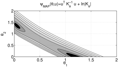
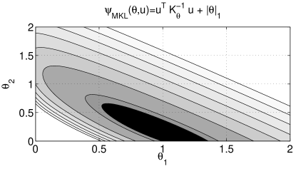
Figure 2: Convex and non-convex building blocks of the MKL and MAP objective function

Intuition for the Gaussian Case

We can gain further intuition about the criteria $\phi_{\text{MKL}}$ and $\phi_{\text{MAP}}$ by asking which matrices $\mathbf{K}$ minimise them. For simplicity, assume that $\mathbb{P}(\mathbf{y}|\mathbf{u})=\mathcal{N}(\mathbf{y}|\mathbf{u},\sigma^{2}\mathbf{I})$ and $n/C=\sigma^{2}$, hence $\ell(\mathbf{y},\mathbf{u})=\frac{1}{\sigma^{2}}\left\|\mathbf{y}-\mathbf{u}\right\|_{2}^{2}$. The inner minimiser $\hat{\mathbf{u}}$ for both $\phi_{\text{MKL}}$ and $\phi_{\text{MAP}}$ is given by $\mathbf{K}_{\bm{\theta}}^{-1}\hat{\mathbf{u}}=(\mathbf{K}_{\bm{\theta}}+\sigma^{2}\mathbf{I})^{-1}\mathbf{y}$. With $\sigma^{2}\to 0$, we find for joint MAP that $\frac{\partial}{\partial\mathbf{K}}\phi_{\text{MAP}}=\mathbf{0}$ results in $\hat{\mathbf{K}}=\mathbf{y}\mathbf{y}^{\top}$. While this “nonparametric” estimate requires smoothing to be useful in practice, closeness to $\mathbf{y}\mathbf{y}^{\top}$ is fundamental to covariance estimation and can be found in regularised risk kernel learning work (Christianini et al., 2001). On the other hand, for $\text{tr}(\mathbf{K}_{m})=1$ and hence $\rho(\bm{\theta})=\lambda\text{tr}(\mathbf{K}_{\bm{\theta}})=\lambda\left\|\bm{\theta}\right\|_{1}$, $\frac{\partial}{\partial\mathbf{K}}\phi_{\text{MKL}}=\mathbf{0}$ leads to $\hat{\mathbf{K}}^{2}=\lambda^{-1}\mathbf{y}\mathbf{y}^{\top}$: an odd way of estimating covariance, not supported by any statistical literature we are aware of.

2.3 Marginal Likelihood Maximisation

While the joint MAP criterion uses a properly normalised prior distribution, it is still not probabilistically consistent. Kernel learning amounts to finding a value $\hat{\bm{\theta}}$ of high data likelihood, no matter what the latent function $u(\cdot)$ is. The correct likelihood to be maximised is marginal: $\mathbb{P}(\mathbf{y}|\bm{\theta})=\int\mathbb{P}(\mathbf{y}|\mathbf{u})\mathbb{P}(\mathbf{u}|\bm{\theta})\text{d}\mathbf{u}$ (“max-sum”), while joint MAP employs the plug-in surrogate $\max_{\mathbf{u}}\mathbb{P}(\mathbf{y}|\mathbf{u})\mathbb{P}(\mathbf{u}|\bm{\theta})$ (“max-max”). Marginal likelihood maximisation (MLM) is also known as Bayesian estimation, and it underlies the EM algorithm or maximum likelihood learning of conditional random fields just as well: complexity is controlled (and overfitting avoided) by averaging over unobserved variables $\mathbf{u}$ (MacKay, 1992), rather than plugging in some point estimate $\hat{\mathbf{u}}$

$$\phi_{\text{MLM}}(\bm{\theta}):=-2\ln\int\mathcal{N}(\mathbf{u}|\mathbf{0},\mathbf{K}_{\bm{\theta}})\mathbb{P}(\mathbf{y}|\mathbf{u})\text{d}\mathbf{u}.$$ (5)

The Gaussian Case

Before developing a general MLM approximation, we note an important analytically solvable exception: for Gaussian likelihood $\mathbb{P}(\mathbf{y}|\mathbf{u})=\mathcal{N}(\mathbf{y}|\mathbf{u},\sigma^{2}\mathbf{I})$, $\mathbb{P}(\mathbf{y}|\bm{\theta})=\mathcal{N}(\mathbf{y}|\mathbf{0},\mathbf{K}_{\bm{\theta}}+\sigma^{2}\mathbf{I})$, and MLM becomes

$$\phi_{\text{GAU}}(\bm{\theta}):=\mathbf{y}^{\top}(\mathbf{K}_{\bm{\theta}}+\sigma^{2}\mathbf{I})^{-1}\mathbf{y}+\ln|\mathbf{K}_{\bm{\theta}}+\sigma^{2}\mathbf{I}|.$$ (6)

Even if the primary purpose is classification, the Gaussian likelihood is used for its analytical simplicity (Kapoor et al., 2009). Only for the Gaussian case, joint MAP and MLM have an analytically closed form. From the product formula of Gaussians (Brookes, 2005, §5.1)

$$\mathbb{Q}(\mathbf{u}):=\mathcal{N}(\mathbf{u}|\mathbf{0},\mathbf{K}_{\bm{\theta}})\mathcal{N}(\mathbf{y}|\mathbf{u},\bm{\Gamma})=\mathcal{N}(\mathbf{y}|\mathbf{0},\mathbf{K}_{\bm{\theta}}+\bm{\Gamma})\mathcal{N}(\mathbf{u}|\mathbf{m},\mathbf{V}),$$

where $\mathbf{V}=(\mathbf{K}_{\bm{\theta}}^{-1}+\bm{\Gamma}^{-1})^{-1}$ and $\mathbf{m}=\mathbf{V}\bm{\Gamma}^{-1}\mathbf{y}$ we can deduce that

$$-2\ln\int\mathbb{Q}(\mathbf{u})\text{d}\mathbf{u}=\ln|\mathbf{K}_{\bm{\theta}}^{-1}+\bm{\Gamma}^{-1}|+\min_{\mathbf{u}}[-2\ln\mathbb{Q}(\mathbf{u})]-n\ln|2\pi|.$$ (7)

Using $\sigma^{2}\mathbf{I}=\bm{\Gamma}$ and $\min_{\mathbf{u}}[-2\ln\mathbb{Q}(\mathbf{u})]=-2\ln\mathbb{Q}(\mathbf{m})$, we see that by

$$\phi_{\text{MAP/GAU}}(\bm{\theta}):\stackrel{{\scriptstyle\text{c}}}{{=}}\phi_{\text{GAU}}(\bm{\theta})-\ln|\mathbf{K}_{\bm{\theta}}^{-1}+\sigma^{-2}\mathbf{I}|\stackrel{{\scriptstyle\text{c}}}{{=}}\mathbf{y}^{\top}(\mathbf{K}_{\bm{\theta}}+\sigma^{2}\mathbf{I})^{-1}\mathbf{y}+\ln|\mathbf{K}_{\bm{\theta}}|$$ (8)

MLM and MAP are very similar for the Gaussian case.

The “ridge regression” approximation is also used together with $p$-norm constraints instead of the $\ln|\mathbf{K}_{\bm{\theta}}|$ term (Cortes et al., 2009)

$$\phi_{\text{RR}}(\bm{\theta}):=\mathbf{y}^{\top}(\mathbf{K}_{\bm{\theta}}+\sigma^{2}\mathbf{I})^{-1}\mathbf{y}+\lambda\left\|\bm{\theta}\right\|_{p}^{p}.$$ (9)

Unfortunately, most GP methods to date work with a Gaussian likelihood for simplicity, a restriction which often proves short-sighted. Gaussian-linear models come with unrealistic properties, and benefits of MLM over joint MAP cannot be realised.

Kernel parameter learning has been an integral part of probabilistic GP methods from the very beginning. Williams and Rasmussen (1996) proposed MLM for Gaussian noise equation 6, fifteen years ago. They treated sums of exponential and linear kernels as well as learning lengthscales (ARD), predating recent proposals such as “products of kernels” (Varma and Babu, 2009).

The General Case

In general, joint MAP always has the analytical form equation 4, while $\mathbb{P}(\mathbf{y}|\bm{\text{$\theta$}})$ can only be approximated. For non-Gaussian $\mathbb{P}(\mathbf{y}|\mathbf{u})$, numerous approximate inference methods have been proposed, specifically motivated by learning kernel parameters via MLM. The simplest such method is Laplace’s approximation, applied to GP binary and multi-way classification by Williams and Barber (1998): starting with convex joint MAP, $\ln\mathbb{P}(\mathbf{y},\mathbf{u})$ is expanded to second order around the posterior mode $\hat{\mathbf{u}}$. More recent approximations Girolami and Rogers (2005); Girolami and Zhong (2006) can be much more accurate, yet come with non-convex problems and less robust algorithms (Nickisch and Rasmussen, 2008). In this paper, we concentrate on the variational lower bound relaxation (VB) by Jaakkola and Jordan (2000), which is convex for log-concave likelihoods $\mathbb{P}(\mathbf{y}|\mathbf{u})$ (Nickisch and Seeger, 2009), providing a novel simple and efficient algorithm. While our VB approximation to MLM is more expensive to run than joint MAP for non-Gaussian likelihood (even using Laplace’s approximation), the implementation complexity of our VB algorithm is comparable to what is required in the Gaussian noise case equation 6.

More, specifically, we exploit that super-Gaussian of likelihoods $\mathbb{P}(y_{i}|u_{i})$ can be lower bounded by scaled Gaussians $\mathcal{N}_{\gamma_{i}}$ of any width $\gamma_{i}$:

$$\mathbb{P}(y_{i}|u_{i})=\max_{\gamma_{i}>0}\mathcal{N}_{\gamma_{i}}=\max_{\gamma_{i}>0}\exp\left(\beta_{i}u_{i}-\frac{u_{i}^{2}}{2\gamma_{i}}-\frac{1}{2}h_{i}(\gamma_{i})\right),$$

where $\beta_{i}\propto y_{i}$ are constants, and $h_{i}(\cdot)$ is convex (Nickisch and Seeger, 2009) whenever the likelihood $\mathbb{P}(y_{i}|u_{i})$ is log-concave. If the posterior distribution is $\mathbb{P}(\mathbf{u}|\mathbf{y})=Z^{-1}\mathbb{P}(\mathbf{y}|\mathbf{u})\mathbb{P}(\mathbf{u})$, then $\ln Z\geq Ce^{-\psi_{\text{VB}}(\bm{\theta},\bm{\gamma})/2}$ by plugging in these bounds, where $C$ is a constant and

$$\phi_{\text{VB}}(\bm{\theta}):=\min_{\bm{\gamma}\succ\mathbf{0}}\psi_{\text{VB}}(\bm{\theta},\bm{\gamma}),\quad\psi_{\text{VB}}(\bm{\theta},\bm{\gamma}):=h(\bm{\gamma})-2\ln\int\mathcal{N}(\mathbf{u}|\mathbf{0},\mathbf{K}_{\bm{\theta}})e^{\mathbf{u}^{\top}(\bm{\beta}-\frac{1}{2}\bm{\Gamma}{}^{-1}\mathbf{u})}\text{d}\mathbf{u},$$ (10)

$h(\bm{\gamma}):=\sum_{i}h_{i}(\gamma_{i})$, $\bm{\Gamma}:=\text{dg}(\bm{\gamma})$. The variational relaxation amounts to maximising the lower bound, which means that $\mathbb{P}(\mathbf{u}|\mathbf{y})$ is fitted by the Gaussian approximation $\mathbb{Q}(\mathbf{u}|\mathbf{y};\bm{\gamma})$ with covariance matrix $\mathbf{V}=(\mathbf{K}_{\bm{\theta}}^{-1}+\bm{\Gamma}{}^{-1})^{-1}$ (Nickisch and Seeger, 2009). Alternatively, we can interpret $\psi_{\text{VB}}(\bm{\theta},\bm{\gamma})$ as an upper bound on the Kullback-Leibler divergence $\text{KL}(\mathbb{Q}(\mathbf{u}|\mathbf{y};\bm{\gamma})||\mathbb{P}(\mathbf{u}|\mathbf{y}))$ (Nickisch, 2010, §2.5.9), a measure for the dissimilarity between the exact posterior $\mathbb{P}(\mathbf{u}|\mathbf{y})$ and the parametrised Gaussian approximation $\mathbb{Q}(\mathbf{u}|\mathbf{y};\bm{\gamma})$.

Finally, note that by equation (7), $\psi_{\text{VB}}(\bm{\theta},\bm{\gamma})$ can also be written as

$$\psi_{\text{VB}}(\bm{\theta},\bm{\gamma})=\ln|\mathbf{K}_{\bm{\theta}}^{-1}+\bm{\Gamma}^{-1}|+h(\bm{\gamma})+\min_{\mathbf{u}}R(\mathbf{u},\bm{\theta},\bm{\gamma})+\ln|\mathbf{K}_{\bm{\theta}}|,$$ (11)

where $R(\mathbf{u},\bm{\theta},\bm{\gamma})=\mathbf{u}^{\top}(\mathbf{K}_{\bm{\theta}}^{-1}+\bm{\Gamma}^{-1})\mathbf{u}-2\bm{\beta}^{\top}\mathbf{u}$. Using the concavity of $\bm{\gamma}^{-1}\mapsto\ln|\mathbf{K}_{\bm{\theta}}^{-1}+\bm{\Gamma}^{-1}|$ and Fenchel duality $\ln|\mathbf{K}_{\bm{\theta}}^{-1}+\bm{\Gamma}^{-1}|=\min_{\mathbf{z}\succ\mathbf{0}}\mathbf{z}^{\top}\bm{\gamma}^{-1}-g_{\bm{\theta}}^{*}(\mathbf{z})=\hat{\mathbf{z}}_{\bm{\theta}}^{\top}\bm{\gamma}^{-1}-g_{\bm{\theta}}^{*}(\hat{\mathbf{z}}_{\bm{\theta}})$, with the optimal value $\hat{\mathbf{z}}_{\bm{\theta}}=\text{dg}(\mathbf{V})$, we can reformulate $\psi_{\text{VB}}(\bm{\theta},\bm{\gamma})$ as

$$\psi_{\text{VB}}(\bm{\theta},\bm{\gamma})=\min_{\mathbf{z}\succ\mathbf{0}}[\mathbf{z}^{\top}\bm{\gamma}^{-1}-g_{\bm{\theta}}^{*}(\mathbf{z})]+h(\bm{\gamma})+\min_{\mathbf{u}}R(\mathbf{u},\bm{\theta},\bm{\gamma})+\ln|\mathbf{K}_{\bm{\theta}}|,$$

which allows to perform the minimisation w.r.t. $\bm{\gamma}$ in closed form (Nickisch, 2010, §3.5.6):

$$\phi_{\text{VB}}(\bm{\theta})=\min_{\mathbf{z}\succ\mathbf{0}}\psi_{\text{VB}}(\bm{\theta},\mathbf{z}),\quad\psi_{\text{VB}}(\bm{\theta},\mathbf{z})=\min_{\mathbf{u}}\mathbf{u}^{\top}\mathbf{K}_{\bm{\theta}}^{-1}\mathbf{u}+\tilde{\ell}_{\mathbf{z}}(\mathbf{y},\mathbf{u})-g_{\bm{\theta}}^{*}(\mathbf{z})+\ln|\mathbf{K}_{\bm{\theta}}|,$$ (12)

where $\tilde{\ell}_{\mathbf{z}}(\mathbf{y},\mathbf{u}):=2\bm{\beta}^{\top}(\mathbf{v}-\mathbf{u})-2\ln\mathbb{P}(\mathbf{y}|\mathbf{v})$ and finally $\mathbf{v}=\text{sign}(\mathbf{u})\odot\sqrt{\mathbf{u}^{2}+\mathbf{z}}$. Note that for $\mathbf{z}=\mathbf{0}$, we exactly recover joint MAP estimation, equation (4), as $\mathbf{z}=\mathbf{0}$ implies $\mathbf{u}=\mathbf{v}$ and $\tilde{\ell}_{\mathbf{z}}(\mathbf{y},\mathbf{u})=\ell(\mathbf{y},\mathbf{u})$. For fixed $\bm{\theta}$, the optimal value $\hat{\mathbf{z}}_{\bm{\theta}}=\text{dg}(\mathbf{V})$ corresponds to the marginal variances of the Gaussian approximation $\mathbb{Q}(\mathbf{u}|\mathbf{y};\bm{\gamma})$: Variational inference corresponds to variance-smoothed joint MAP estimation (Nickisch, 2010) with a loss function $\tilde{\ell}(\mathbf{y},\mathbf{u},\bm{\theta})$ that explicitly depends on the kernel parameters $\bm{\theta}$. We have two equivalent representations of the loss $\tilde{\ell}(\mathbf{y},\mathbf{u},\bm{\theta})$ that directly follow from equations (11) and (12):

$$\tilde{\ell}(\mathbf{y},\mathbf{u},\bm{\theta}) = \min_{\bm{\gamma}\succ\mathbf{0}}[\ln|\mathbf{K}_{\bm{\theta}}^{-1}+\bm{\Gamma}^{-1}|+h(\bm{\gamma})+\mathbf{u}^{\top}\bm{\Gamma}^{-1}\mathbf{u}-2\bm{\beta}^{\top}\mathbf{u}],\>\text{and}$$

$$\tilde{\ell}(\mathbf{y},\mathbf{u},\bm{\theta}) = \min_{\mathbf{z}\succ\mathbf{0}}[2\bm{\beta}^{\top}(\mathbf{v}-\mathbf{u})-2\ln\mathbb{P}(\mathbf{y}|\mathbf{v})-g_{\bm{\theta}}^{*}(\mathbf{z})],\;\mathbf{v}=\text{sign}(\mathbf{u})\odot\sqrt{\mathbf{u}^{2}+\mathbf{z}}.$$

Our VB problem is $\min_{\bm{\theta}\succeq\mathbf{0},\bm{\gamma}\succ\mathbf{0}}\psi_{\text{VB}}(\bm{\theta},\bm{\gamma})$ or equivalently $\min_{\bm{\theta}\succeq\mathbf{0},\mathbf{z}\succ\mathbf{0}}\psi_{\text{VB}}(\bm{\theta},\mathbf{z})$. The inner variables here are $\bm{\gamma}$ and $\mathbf{z}$, in addition to $\mathbf{u}$ in joint MAP. There are further similarities: since $\psi_{\text{VB}}(\bm{\theta},\bm{\gamma})=-2\ln\int e^{-R(\mathbf{u},\bm{\gamma},\bm{\theta})}\text{d}\mathbf{u}+h(\bm{\gamma})+\ln|2\pi\mathbf{K}_{\bm{\theta}}|$, $(\bm{\gamma},\bm{\theta})\mapsto\psi_{\text{VB}}-\ln|\mathbf{K}_{\bm{\theta}}|$ is jointly convex for $\bm{\gamma}\succ\mathbf{0}$, $\bm{\theta}\succeq\mathbf{0}$, by the joint convexity of $(\mathbf{u},\bm{\gamma},\bm{\theta})\mapsto R$ and Prékopa’s theorem (Boyd and Vandenberghe, 2002, §3.5.2). Joint MAP and VB share the same convexity structure. In contrast, approximating $\mathbb{P}(\mathbf{y}|\bm{\theta})$ by other techniques like Expectation Propagation (Minka, 2001) or general Variational Bayes (Opper and Archambeau, 2009) does not even constitute convex problems for fixed $\bm{\theta}$.

2.4 Summary and Taxonomy

Name	Objective function
Marginal Likelihood Maximisation	$\phi_{\text{MLM}}(\bm{\theta})=-2\ln\left[\int\mathcal{N}(\mathbf{u}|\mathbf{0},\mathbf{K}_{\bm{\theta}})\mathbb{P}(\mathbf{y}|\mathbf{u})\text{d}\mathbf{u}\right]$
Variational Bounds	$\phi_{\text{VB}}(\bm{\theta})=\min_{\bm{\gamma}\succ\mathbf{0}}\psi_{\text{VB}}(\bm{\theta},\bm{\gamma})\geq\phi_{\text{MLM}}(\bm{\theta})$ by $\mathbb{P}(y_{i}|u_{i})\geq\mathcal{N}_{\gamma_{i}}$
Maximum A Posteriori	$\phi_{\text{MAP}}(\bm{\theta})=-2\ln\left[\max_{\mathbf{u}}\mathcal{N}(\mathbf{u}|\mathbf{0},\mathbf{K}_{\bm{\theta}})\mathbb{P}(\mathbf{y}|\mathbf{u})\right]=\psi_{\text{VB}}(\bm{\theta},\mathbf{z}=\mathbf{0})$
Multiple Kernel Learning	$\phi_{\text{MKL}}(\bm{\theta})=\phi_{\text{MAP}}(\bm{\theta})+\lambda\left\|\bm{\theta}\right\|_{p}^{p}-\ln|\mathbf{K}_{\bm{\theta}}|=\psi_{\text{MAP}}(\bm{\theta},\bm{\lambda}=\lambda\cdot\mathbf{1})$

	General $\mathbb{P}(y_{i}|u_{i})$		Gaussian $\mathbb{P}(y_{i}|u_{i})$
	$\phi_{\text{MLM}}(\bm{\theta})$, eq. (5)	$\longrightarrow$	$\phi_{\text{GAU}}(\bm{\theta})$, eq. (6)
Super-Gaussian Bounding	$\downarrow$		$\downarrow$	Bound is tight
	$\phi_{\text{VB}}(\bm{\theta})$, eq. (10)	$\longrightarrow$	$\phi_{\text{GAU}}(\bm{\theta})$, eq. (6)
Maximum instead of integral	$\downarrow$		$\downarrow$	Mode $\equiv$ mean
	$\phi_{\text{MAP}}(\bm{\theta})$, eq. (4)	$\longrightarrow$	$\phi_{\text{MAP/GAU}}(\bm{\theta})$, eq. (8)
Bound $\ln|\mathbf{K}_{\bm{\theta}}|\leq\lambda\left\|\bm{\theta}\right\|_{p}^{p}-g^{*}(\lambda\mathbf{1})$	$\downarrow$		$\downarrow$
	$\phi_{\text{MKL}}(\bm{\theta})$, eq. (3)	$\longrightarrow$	$\phi_{\text{RR}}(\bm{\theta})$, eq. (9)

Table 2: Taxonomy of kernel learning objective functions

The upper table visualises the relationship between several kernel learning objective functions for arbitrary likelihood/loss functions: Marginal likelihood maximisation (MLM) can be bounded by variational bounds (VB) and maximum a posteriori estimation (MAP) is a special case $\mathbf{z}=\mathbf{0}$ thereof. Finally multiple kernel learning (MKL) can be understood as an upper bound to the MAP estimation objective $\bm{\lambda}=\lambda\cdot\mathbf{1}$. The lower table complements the upper table by also covering the analytically important Gaussian case.

In the last paragraphs, we have detailed how a variety of kernel learning approaches can be obtained from Bayesian marginal likelihood maximisation in a sequence of nested upper bounding steps. Table 2.4 nicely illustrates how many kernel learning objectives are related to each other – either by upper bounds or by Gaussianity assumptions. We can clearly see, that $\phi_{\text{VB}}(\bm{\theta})$ – as an upper bound to the negative log marginal likelihood – can be seen as the mother function. For a special case, $\mathbf{z}=\mathbf{0}$, we obtain joint maximum a posteriori estimation, where the loss functions does not depend on the kernel parameters. Going further, a particular instance $\bm{\lambda}=\lambda\cdot\mathbf{1}$ yields the widely use multiple kernel learning objective that becomes convex in the kernel parameters $\bm{\theta}$. In the following, we will concentrate on the optimisation and computational similarities between the approaches.

3 Algorithms

In this section, we derive a simple, provably convergent and efficient algorithm for MKL, joint MAP and VB. We use the Lagrangian form of equation (3) and $\ell(\mathbf{y},\mathbf{u}):=-2\ln\mathbb{P}(\mathbf{y}|\mathbf{u})$:

$$\psi_{\text{MKL}}(\bm{\theta},\mathbf{u}) = \mathbf{u}^{\top}\mathbf{K}^{-1}\mathbf{u}+\qquad\;\ell(\mathbf{y},\mathbf{u})\qquad\qquad\qquad\qquad\qquad\;\,+\lambda\cdot\mathbf{1}^{\top}\bm{\theta},\>\lambda>0,$$

$$\psi_{\text{MAP}}(\bm{\theta},\mathbf{u}) = \mathbf{u}^{\top}\mathbf{K}_{\bm{\theta}}^{-1}\mathbf{u}+\qquad\;\ell(\mathbf{y},\mathbf{u})\qquad\qquad\qquad\qquad\qquad\;\,+\ln|\mathbf{K}_{\bm{\theta}}|,\quad\text{and}$$

$$\psi_{\text{VB}}(\bm{\theta},\mathbf{u}) = \mathbf{u}^{\top}\mathbf{K}_{\bm{\theta}}^{-1}\mathbf{u}+\min_{\mathbf{z}\succ\mathbf{0}}\left[\ell(\mathbf{y},\mathbf{v})+2\bm{\beta}^{\top}(\mathbf{v}-\mathbf{u})-g_{\bm{\theta}}^{*}(\mathbf{z})\right]+\ln|\mathbf{K}_{\bm{\theta}}|,$$

$$\qquad\qquad\qquad\qquad\qquad\qquad\qquad\qquad\quad\text{where}\;\mathbf{v}=\text{sign}(\mathbf{u})\odot\sqrt{\mathbf{u}^{2}+\mathbf{z}}.$$

Many previous algorithms use alternating minimization, which is easy to implement but tends to converge slowly. Both $\phi_{\text{VB}}$ and $\phi_{\text{MAP}}$ are jointly convex up to the concave $\bm{\theta}\mapsto\ln|\mathbf{K}_{\bm{\theta}}|$ part. Since $\ln|\mathbf{K}_{\bm{\theta}}|=\min_{\bm{\lambda}\succ\mathbf{0}}\bm{\lambda}^{\top}\bm{\theta}-f^{*}(\bm{\lambda})$ (Legendre duality, Boyd and Vandenberghe, 2002), joint MAP becomes $\min_{\bm{\lambda}\succ\mathbf{0},\bm{\theta}\succeq\mathbf{0},\mathbf{u}}\phi_{\bm{\lambda}}(\bm{\theta},\mathbf{u})$ with $\phi_{\bm{\lambda}}:=\mathbf{u}^{\top}\mathbf{K}_{\bm{\theta}}^{-1}\mathbf{u}+\ell(\mathbf{y},\mathbf{u})+\bm{\lambda}^{\top}\bm{\theta}-f^{*}(\bm{\lambda})$ which is jointly convex in $(\bm{\theta},\mathbf{u})$. Algorithm 1 iterates between refits of $\bm{\lambda}$ and joint Newton updates of $(\bm{\theta},\mathbf{u})$.

0:  Criterion $\psi_{\#}(\bm{\theta},\mathbf{u})=\tilde{\psi}_{\#}(\bm{\theta},\mathbf{u})+\ln|\mathbf{K}_{\bm{\theta}}|$ to minimise for $(\mathbf{u},\bm{\theta})\in\mathbb{R}^{n}\times\mathbb{R}_{+}^{M}$.

  repeat

     Newton $\min_{\mathbf{u}}\psi_{\#}$ for fixed $\bm{\theta}$ (optional; few steps).

     Refit upper bound: $\bm{\lambda}\leftarrow\nabla_{\bm{\theta}}\ln|\mathbf{K}_{\bm{\theta}}|=[\text{tr}(\mathbf{K}_{\bm{\theta}}^{-1}\mathbf{K}_{1}),..,\text{tr}(\mathbf{K}_{\bm{\theta}}^{-1}\mathbf{K}_{M})]^{\top}$.

     Compute joint Newton search direction $\mathbf{d}$ for $\psi_{\bm{\lambda}}:=\tilde{\psi}_{\#}+\bm{\lambda}^{\top}\bm{\theta}$:     $\nabla_{[\bm{\theta};\mathbf{u}]}^{2}\psi_{\bm{\lambda}}\mathbf{d}=-\nabla_{[\bm{\theta};\mathbf{u}]}\psi_{\bm{\lambda}}$.

     Linesearch: Minimise $\psi_{\#}(\alpha)$ i.e. $\psi_{\#}(\bm{\theta},\mathbf{u})$ along $[\bm{\theta};\mathbf{u}]+\alpha\mathbf{d}$, $\alpha>0$.

  until Outer loop converged

Algorithm 1 Double loop algorithm for joint MAP, MKL and VB.

The Newton direction costs $O(n^{3}+M\,n^{2})$, with $n$ the number of data points and $M$ the number of base kernels. All algorithms discussed in this paper require $O(n^{3})$ time, apart from the requirement to store the base matrices $\mathbf{K}_{m}$. The convergence proof hinges on the fact that $\phi$ and $\phi_{\bm{\lambda}}$ are tangentially equal (Nickisch and Seeger, 2009). Equivalently, the algorithm can be understood as Newton’s method, yet dropping the part of the Hessian corresponding to the $\ln|\mathbf{K}|$ term (note that $\nabla_{(\mathbf{u},\bm{\theta})}\phi_{\bm{\lambda}}=\nabla_{(\mathbf{u},\bm{\theta})}\phi$ for the Newton direction computation). Exact Newton for MKL.

In practice, we use $\mathbf{K}_{\bm{\theta}}=\sum_{m}\theta_{m}\mathbf{K}_{m}+\varepsilon\mathbf{I},\>\varepsilon=10^{-8}$ to avoid numerical problems when computing $\bm{\lambda}$ and $\ln|\mathbf{K}_{\bm{\theta}}|$. We also have to enforce $\bm{\theta}\succeq\mathbf{0}$ in algorithm 1, which is done by the barrier method (Boyd and Vandenberghe, 2002). We minimise $t\phi+\mathbf{1}^{\top}(\ln\bm{\theta})$ instead of $\phi$, increasing $t>0$ every few outer loop iterations.

A variant algorithm 1 can be used to solve VB in a different parametrisation ($\bm{\gamma}\succ\mathbf{0}$ replaces $\mathbf{u}$), which has the same convexity structure as joint MAP. Transforming equation (10) similarly to equation (6), we obtain

$$\phi_{\text{VB}}(\bm{\theta})=\min_{\bm{\gamma}\succ\mathbf{0}}\ln|\mathbf{C}|-\ln|\bm{\Gamma}|+\bm{\beta}^{\top}\bm{\Gamma}\mathbf{C}^{-1}\bm{\Gamma}\bm{\beta}-\bm{\beta}^{\top}\bm{\Gamma}\bm{\beta}+h(\bm{\gamma})$$ (13)

with $\mathbf{C}:=\mathbf{K}_{\bm{\theta}}+\bm{\Gamma}$, computed using the Cholesky factorisation $\mathbf{C}=\mathbf{L}\mathbf{L}{}^{\top}$. They cost $O(M\,n^{3})$ to compute, which is more expensive than for joint MAP or MKL. Note that the cost $O(M\,n^{3})$ is not specific to our particular relaxation or algorithm e.g. the Laplace MLM approximation (Williams and Barber, 1998), solved using gradients w.r.t. $\bm{\theta}$ only, comes with the same complexity.

4 Conclusion

We presented a unifying probabilistic viewpoint to multiple kernel learning that derives regularised risk approaches as special cases of approximate Bayesian inference. We provided an efficient and provably convergent optimisation algorithm suitable for regression, robust regression and classification.

Our taxonomy of multiple kernel learning approaches connected many previously only loosely related ideas and provided insights into the common structure of the respective optimisation problems. Finally, we proposed an algorithm to solve the latter efficiently.

References

• Bach et al. (2004) Francis Bach, Gert Lanckriet, and Michael Jordan. Multiple kernel learning, conic duality, and the SMO algorithm. In ICML, 2004.
• Boyd and Vandenberghe (2002) Stephen Boyd and Lieven Vandenberghe. Convex Optimization. Cambridge University Press, 2002.
• Brookes (2005) Mike Brookes. The matrix reference manual, 2005. URL http://www.ee.ic.ac.uk/hp/staff/dmb/matrix/intro.html.
• Christianini et al. (2001) Nello Christianini, John Shawe-Taylor, André Elisseeff, and Jaz Kandola. On kernel-target alignment. In NIPS, 2001.
• Cortes et al. (2009) Corinna Cortes, Mehryar Mohri, and Afshin Rostamizadeh. L2 regularization for learning kernels. In UAI, 2009.
• Girolami and Rogers (2005) Mark Girolami and Simon Rogers. Hierarchic Bayesian models for kernel learning. In ICML, 2005.
• Girolami and Zhong (2006) Mark Girolami and Mingjun Zhong. Data integration for classification problems employing Gaussian process. In NIPS, 2006.
• Jaakkola and Jordan (2000) Tomi Jaakkola and Michael Jordan. Bayesian parameter estimation via variational methods. Statistics and Computing, 10:25–37, 2000.
• Kapoor et al. (2009) Ashish Kapoor, Kristen Grauman, Raquel Urtasun, and Trevor Darrell. Gaussian processes for object categorization. IJCV, 2009. doi: 10.1007/s11263-009-0268-3.
• Kloft et al. (2009) Marius Kloft, Ulf Brefeld, Sören Sonnenburg, Pavel Laskov, Klaus-Robert Müller, and Alexander Zien. Efficient and accurate lp-norm multiple kernel learning. In NIPS, 2009.
• Lanckriet et al. (2004) Gert R. G. Lanckriet, Nello Cristianini, Peter Bartlett, Laurent El Ghaoui, and Michal I. Jordan. Learning the kernel matrix with semidefinite programming. JMLR, 5:27–72, 2004.
• MacKay (1992) Davic MacKay. Bayesian interpolation. Neural Computation, 4(3):415–447, 1992.
• Minka (2001) Tom Minka. Expectation propagation for approximate Bayesian inference. In UAI, 2001.
• Mishra and Giorgi (2008) Shashi Kant Mishra and Giorgio Giorgi. Invexity and optimization. Springer, 2008.
• Nickisch (2010) Hannes Nickisch. Bayesian Inference and Experimental Design for Large Generalised Linear Models. PhD thesis, TU Berlin, 2010.
• Nickisch and Rasmussen (2008) Hannes Nickisch and Carl Edward Rasmussen. Approximations for binary Gaussian process classification. JMLR, 9:2035–2078, 2008.
• Nickisch and Seeger (2009) Hannes Nickisch and Matthias Seeger. Convex variational Bayesian inference for large scale generalized linear models. In ICML, 2009.
• Opper and Archambeau (2009) Manfred Opper and Cédric Archambeau. The variational Gaussian approximation revisited. Neural Computation, 21(3):786–792, 2009.
• Rasmussen and Williams (2006) Carl Edward Rasmussen and Christopher K. I. Williams. Gaussian Processes for Machine Learning. MIT Press, 2006.
• Schölkopf and Smola (2002) Bernhard Schölkopf and Alex Smola. Learning with Kernels. MIT Press, 1st edition, 2002.
• Sollich (2000) Peter Sollich. Probabilistic methods for support vector machines. In NIPS, 2000.
• Sonnenburg et al. (2006) Sören Sonnenburg, Gunnar Rätsch, Christin Schäfer, and Bernhard Schölkopf. Large scale multiple kernel learning. JMLR, 7:1531–1565, 2006.
• Varma and Babu (2009) Manik Varma and Bodla Rakesh Babu. More generality in efficient multiple kernel learning. In ICML, 2009.
• Varma and Ray (2007) Manik Varma and Debajyoti Ray. Learning the discriminative power-invariance trade-off. In ICCV, 2007.
• Williams and Barber (1998) Christopher K. I. Williams and David Barber. Bayesian classification with Gaussian processes. IEEE Transactions on Pattern Analysis and Machine Intelligence, 20(12):1342–1351, 1998.
• Williams and Rasmussen (1996) Christopher K. I. Williams and Carl Edward Rasmussen. Gaussian processes for regression. In NIPS, 1996.
• Zhang (2010) Tong Zhang. Analysis of multi-stage convex relaxation for sparse regularization. JMLR, 11:1081–1107, 2010.