A New Simple Method for the Analysis of Extensive Air Showers

Abstract

The most important goal of studying an extensive air shower is to find the energy, mass and arrival direction of its primary cosmic ray. In order to find these parameters, the core position and arrival direction of the shower should be determined. In this paper, a new method for finding core location has been introduced that utilizes trigger time information of particle detectors. We have also developed a simple technique to reconstruct the arrival direction. Our method is not based upon density-sensitive detectors which are sensitive to the number of crossing particles and is also independent of lateral distribution models. This model has been developed and examined by the analysis of simulated shower events generated by the CORSIKA package.

1 Introduction

An Extensive Air Shower (EAS) is a large number of secondary particles originating from a high energy primary cosmic particle. A lot of efforts have been made to understand the structure and development of EASs. For an accurate investigation of the EAS events, we first have to know their direction and core position. The better the measurement of these parameters, the more precise the exploration of extensive air shower structures. Plane Wave Front Approximation (PWFA) is the simplest way to find the direction of EAS, and spherical front approximation [1] is a complementary approach to obtain more accurate results. The common method for finding core locations of extensive air showers is to fit a Lateral Density Function (LDF) to the density of secondary particles of the shower. Greisen function [2] and its modified form (e.g. [3]) are usually used as LDF. In LDF methods, one uses the particle density information without considering their arrival time information.
Some attempts have been made to use mean arrival time and disk thickness as a measure of the shower core distance [4]. Measurements of the EAS disk structure were tried by Bassi, Clark, and Rossi in 1953 [5] and continued later [6]. However, it has recently been shown that both mean arrival time and EAS front thickness in individual showers fluctuate strongly and cannot be a good measure of the distance from the EAS axis [7].
Though, due to the strong fluctuations, arrival time cannot be used as a measure of the distance from the core, it can be used to provide a statistical analysis for some of the EAS features. In this paper, we propose a model independent approach for finding core location and arrival direction of EASs which uses arrival time information, avoids using LDF and can be used for arrays lacking Density Sensitive Detectors (DSDs), which are sensitive to density or to the number of crossing particles. In order to examine the capability of the method, we used the CORSIKA [8] package.

2 Physical Principles

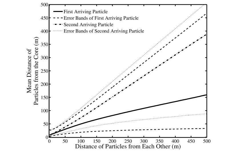
Figure 1: Average distance of the first arriving particle (solid curve) and the second arriving particle (dash-dot curve) from the core versus their distance from each other for all secondary charged particles of the showers. The related error bands are also depicted. The results have been reached by additional 10,000 vertical single energy (100 TeV) showers generated by CORSIKA. The low energy hadronic model is FLUKA [9, 10] and the high energy hadronic model is QGSJETII [11, 12].

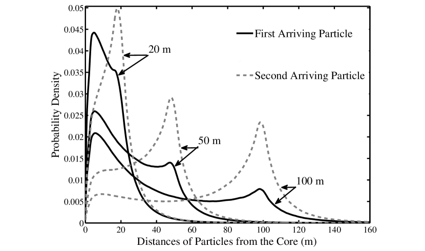
Figure 2: Probability density of distances of two typical particles of those EASs which were used in Fig. 1. Three groups of particle couples were selected with separations of 20 m $\pm$ 0.5 m, 50 m $\pm$ 0.5 m and 100 m $\pm$ 0.5 m. Solid lines belong to the first arriving particles and dashed lines belong to the second arriving particles. In all three cases the first arriving particle is more probable to be closer to the core.

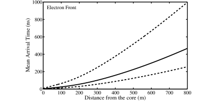
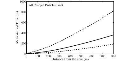
Figure 3: Mean arrival times of particles versus the distance from the core for the same showers which were used in Fig. 1. Dashed lines are error bands.

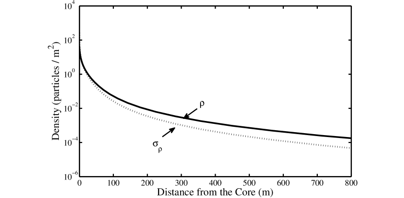
Figure 4: The lateral density of charged particles, $\rho$, and its standard deviation, $\sigma_{\rho}$, versus the distance from the core for the VEASs used in Fig. 1.

An important feature of EASs is their spherical front, which is approximately a spherical cap. Thus the particles in the core region of a Vertical EAS (VEAS) reach to the ground level sooner than in other regions. This feature can be demonstrated by considering the fact that if we randomly select any two secondary particles of a VEAS, the first particle reaching ground level on average is closer to the core location. Fig. 1 shows that by increasing the distance between two particles, the average distance of the first arriving particle from the core increases slowly, while the average distance of the second particle from the core increases rather rapidly.
Another feature of EASs is that the particle density in the core neighborhood is larger than in other regions. The smaller the distance between two particles, the smaller their distance to the core on average, as also follows from Fig. 1. Error bands also have been depicted in order to show the fluctuations. They have been derived by calculating the RMS for positive and negative errors separately. As can be seen the error bands are asymmetric. Fig. 2 shows the reason of this asymmetry.
The peak structures in Fig. 2 show that the first arriving particle to the ground level is more likely to be closer to the core location. For the small separations of particles, both probability density functions have a unique pronounced peak close to the core region. So, when the separation of two particles is small, it is quite probable that both particles to be in approximately equal distance from the core in opposite sides. For larger separations, both probability densities have two peaks, one of which is higher than the other. For the first arriving particle, the higher maximum is near the core region, but the other one has the same distance from the core as the distance between two particles. For the second particle the situation is vice versa. So, when their distances increase, although there is a small probability that the first arriving particle will be found farther from the core than the second one, it is more probable that the first arriving particle to be much closer to the core region than the second arriving particle.
The density of secondary particles quickly decreases by increasing the distance from the core in contrast to the slow increase of the average arrival time of particles shown in Fig. 3. A rough investigation shows that random fluctuation of the density of the particles is much less than their arrival time fluctuations, especially when they are far from the core. Fig. 4 shows that the fluctuation of lateral density of the particles decreases with the core distance rapidly in contrast to the arrival time fluctuation which increases with the core distance (Fig. 3). So if we want to choose between particle density information and arrival time information as a measure of the core location, the particle density information is a more decisive factor.

3 A Method for Finding Core Location

A simple approximate method to find the core position of an EAS is to calculate the Center of Gravity (CG) of the Triggered Detectors (TDs) which is a relatively good approximation for those EASs whose cores are very close to the center of the array. We have introduced a procedure which is capable to increase the precision of CG for finding the approximate location of the core even when the core position is close to the border of the array.
At first, we assume that every detector can just detect the first crossing particle and is unable to detect any other particle during an event. For simplicity, we investigated VEAS events at first and then generalized the results to the inclined EASs.
Assume that we have positions and trigger times of all TDs of an array during a VEAS event. TDs are indexed based on their trigger times, starting with $i=1$ for the first TD. Fig. 3 suggests that if $i<j<k$ then $\langle r_{i}\rangle<\langle r_{j}\rangle<\langle r_{k}\rangle$, where $\langle r_{i}\rangle$ is the average distance of the $i$th TD to the shower core. Therefore, by taking into account Fig. 1, this result can be achieved: $\langle d_{ij}\rangle<\langle d_{ik}\rangle$ (where $d_{ij}=|\vec{r}_{i}-\vec{r}_{j}|$). If we want to find the nearest detector to the core, selecting the $i$th detector seems to be logical, but because of timing fluctuations, a better choice will be obtained by the following procedure: At first, we find the minimum value of $d_{ij}$, $d_{ik}$ and $d_{jk}$. If $d_{jk}$ is the smallest value then the $j$th detector is most likely nearest to the core, since $j<k$.

3.1 SIMEFIC Algorithm

Based on the principles explained above, we developed the SIMEFIC (SIeving MEthod for FInding Core) algorithm for eliminating detectors far from the core. Let us assume that there are $N$ TDs in an array during a VEAS. We form a matrix $D_{N\times N}$, whose elements are $d_{ij}$s. In view of the fact that $D$ is a symmetric matrix, we just consider the upper triangle of the matrix without principal diagonal elements, which are zero.

$$D=\left(\begin{array}[]{ccccc}\times&d_{12}&d_{13}&\cdots&d_{1N}\\ \times&\times&d_{23}&\cdots&d_{2N}\\ \times&\times&\times&\cdots&d_{3N}\\ \vdots&\vdots&\vdots&\ddots&\vdots\\ \times&\times&\times&\cdots&\times\\ \end{array}\right)$$

Then we can find the smallest element ($d_{<}$) under the following two conditions:

If $d_{ij}=d_{kl}$ and $i<k$ then $d_{<}=d_{ij}$

If $d_{ij}=d_{ik}$ and $j<k$ then $d_{<}=d_{ij}$

Now we select the $i$th TD as the first detector of our near-core list (because of its trigger time). Next, in the $i$th row, we find the biggest element ($d_{>}$) under the following condition:

If all $d_{ij}$s ($j=i+1,...,N$) are different, the biggest element, e.g. $d_{ik}$, is $d_{>}$, and if $d_{ij}$ and $d_{ik}$ are both the biggest elements ($d_{ij}=d_{ik}$), and $j<k$ then $d_{>}=d_{ik}$.

We now eliminate the $k$th TD as an off-core detector and remove the $i$th and $k$th rows and columns of the matrix $D$ . By repeating this procedure for the reduced matrix ($D_{N-2\times N-2}$), we will reach a position in which half of the TDs are retained and half of them are eliminated. Now, it is expected that the CG of the retained TDs is a good measure of the core location.

3.1.1 Inclined showers

Up to now, our discussion was limited to the VEASs. To generalize this method to inclined EASs, the detector coordinates, and also the trigger times need to be transformed into the coordinate system of the shower. The coordinates of the detectors on the ground level are $x_{i}$, $y_{i}$, and $z_{i}=0$. Now, these coordinates are transformed to a new coordinate system whose $x$ and $y$ axes are perpendicular to the arrival direction. To perform this, we select an arbitrary point (e.g. the CG of all detectors) as the origin of coordinate system. Then the coordinates of the detectors are first rotated counterclockwise around the $z$ axis by the angle $\phi$ and next the new coordinates are rotated clockwise around the $y^{{}^{\prime}}$ by the angle $\theta$. The $z$ components in the final coordinate system are $z_{i}^{{}^{\prime\prime}}=-x_{i}\sin\theta\cos\phi-y_{i}\sin\theta\sin\phi$. Accordingly the trigger times of the detectors are transformed to $t_{i}^{{}^{\prime\prime}}=t_{i}+z_{i}^{{}^{\prime\prime}}/c$ where c is the speed of light. Now the inclined showers are treated as the vertical ones.

3.1.2 Arrays of DSDs

For arrays with DSDs the algorithm is extended as follows. Another matrix, $N$, is formed, the elements of which are $n_{ij}=n_{i}+n_{j}$ ($n_{i}$ is the number of the detected particles by $i$th detector) in correspondence with $d_{ij}$ elements of the matrix $D$. Now, we first select a pair of detectors with maximum $n_{ij}$ ($n_{max}$) under the following two conditions:

If $n_{ij}=n_{kl}$ with $i<k$, and if $d_{ij}>d_{kl}$, then $n_{max}=n_{kl}$ and if $d_{ij}\leq d_{kl}$, then $n_{max}=n_{ij}$.

If $n_{ij}=n_{ik}$ with $j<k$, and if $d_{ij}>d_{ik}$, then $n_{max}=n_{ik}$ and if $d_{ij}\leq d_{ik}$, then $n_{max}=n_{ij}$.

Assume that $n_{ij}$ has been selected as $n_{max}$ and $n_{i}<n_{j}$, then $j$ is the near core detector (if $n_{i}>n_{j}$, $i$th detector will be chosen). If $n_{i}=n_{j}$, the trigger times of the two detectors $i$ and $j$ will be the determining factor for choosing between $i$ and $j$ as the near core detector. Other stages of the algorithm are the same as before.

3.2 Reconstruction of a Shower Geometry

As the precision of final results of SIMEFIC algorithm is tied to the precision of arrival direction measurement, a method has been introduced here that can be used for more precise arrival direction reconstruction.
Assume that we have $\{P_{i}\}$ set of the locations and trigger times of all TDs at the beginning of the calculation. By using PWFA and SIMEFIC algorithm on the set $\{P_{i}\}$, a subset of it, $\{P_{i}^{{}^{\prime}}\}$, will be found whose members are half of the first set. Now, PWFA is used in shower direction reconstruction of the $\{P_{i}^{{}^{\prime}}\}$ set from which the arrival direction is calculated with more precision. The reason for higher precision, of this technique in comparison with the PWFA used for the set $\{P_{i}\}$, is that arrival times have less fluctuation in near core region than those in far regions from the core. Furthermore, the front of an EAS is smoother in near core region than that in far regions. In view of these facts, SIMEFIC method presents a better approximation for arrival direction in comparison with the PWFA, which uses data of all TDs. Now, we propose a refinement to the SIMEFIC method by repetition of the above procedure:

1. Reconstruct arrival direction by using $\{P_{i}^{{}^{\prime}}\}$ set with PWFA, $(\theta^{{}^{\prime}},\phi^{{}^{\prime}})$.

2. Use SIMEFIC algorithm for the original set, $\{P_{i}\}$ (not on set $\{P_{i}^{{}^{\prime}}\}$ which has $N/2$ members) and arrival direction $(\theta^{{}^{\prime}},\phi^{{}^{\prime}})$, to obtain another set $\{P_{i}^{{}^{\prime\prime}}\}$.

3. Replace $\{P_{i}^{{}^{\prime}}\}$ by $\{P_{i}^{{}^{\prime\prime}}\}$ and repeat the procedure.

This procedure is repeated several times using the original set to refine the arrival direction. If two successive runs yield approximately the same results, the process will be terminated. In our simulation, repeating for 3 times was enough.

4 Simulations with CORSIKA

The geographical coordinates of the prototype of Alborz observatory location (in Tehran, $35^{\circ}$N, $51^{\circ}$E and 1200 m above sea level) have been imposed in CORSIKA EAS simulations. Geomagnetic field components of Tehran are $B_{x}=28.1\mu$T and $B_{z}=38.4\mu$T. For the simulation of low energy hadronic interactions, GHEISHA [13] package, and for high energy cases QGSJET01 package have been used. Zenith angles of primary particles were chosen between $0^{\circ}$ and $60^{\circ}$. The compositions of primary particles have been $90\%$ protons and $10\%$ helium nuclei. This ratio was assumed to be constant over entire energy range. The energy of the primary particles ranges from 100 TeV to 5 PeV. Other parameters are CORSIKA default values (e.g. default spectrum index of $-2.7$).
The assumed array is a square with an area of $200\times 200$ m², composed of $1\times 1$ m² detectors on a square lattice with a $5$ m lattice constant (total of $41\times 41$ detectors). Ground arrays are commonly made up of scintillation detectors which are not sensitive to the position of the crossing particles and are not able to exactly measure how many particles have passed through them. Therefore, the following assumptions have been applied for the simulation.
When the first arriving particle passes through a detector, its arrival time is considered as the trigger time of that detector. Obviously, the coordinates of this first crossing particle must be within $\pm 0.5$ m of the center of the detector in order to consider the detector as a TD. The next arriving particles which pass through this hypothetical detector are not taken into account.
The CG of TDs for the array whose detectors are DSDs will be considered as follows:

$$x_{CG} =1/N\displaystyle\sum\limits_{i}n_{i}x_{i},$$

$$y_{CG} =1/N\displaystyle\sum\limits_{i}n_{i}y_{i}$$

where $n_{i}$ is the pulse height (the number of crossing particles) of each detector and $N=\displaystyle\sum\limits_{i}n_{i}$. For non DSDs, we set $n_{i}=1$ for all TDs.
If the coordinates of the EAS true core are denoted by $(x_{tc},y_{tc})$, the distance between the true core and the CG will be:

$$r=\sqrt{(x_{CG}^{{}^{\prime\prime}}-x_{tc}^{{}^{\prime\prime}})^{2}+(y_{CG}^{{}^{\prime\prime}}-y_{tc}^{{}^{\prime\prime}})^{2}}$$

where $x^{{}^{\prime\prime}},y^{{}^{\prime\prime}}$ are coordinates in the rotated coordinate system introduced in sec. 3.1.1.

4.1 Results

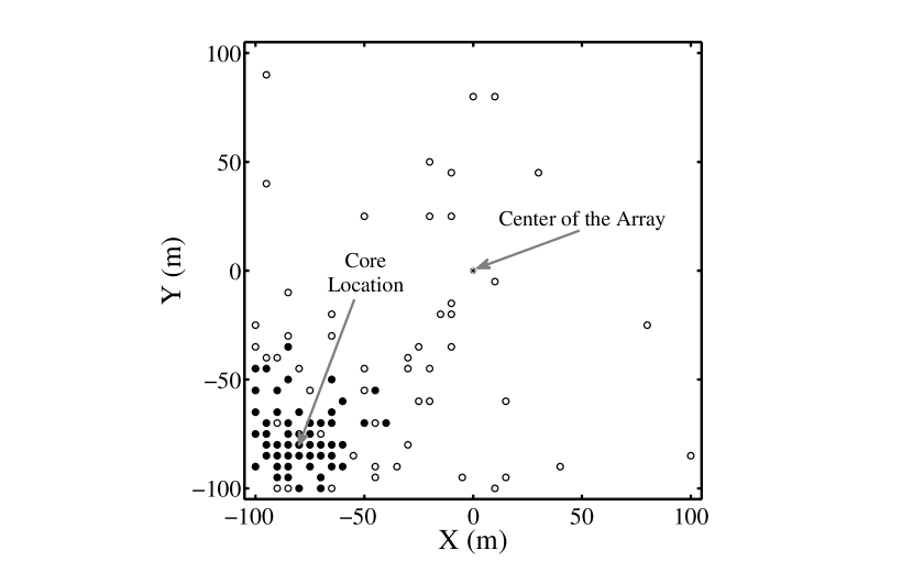
Figure 5: The TDs which are accepted by SIMEFIC method are shown by the bold circles and the omitted ones by the empty circles. The position of the true core and the center of the array have been shown. The zenith and azimuth angles of this shower are $29.5^{\circ}$ and $329.5^{\circ}$ respectively, and its energy is 157.5 TeV.

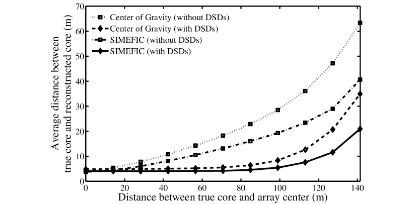
Figure 6: The comparison of the CG of all TDs and those which have been selected by SIMEFIC. The size of error bars for each data point is less than the size of the symbols used for them.

Fig. 5 shows an EAS which its true core is on point $(-80,-80)$. Detectors accepted by SIMEFIC method are shown by the bold circles and the omitted ones by the empty circles. It is clear that even when the true core is near the edge of the array, this algorithm has approximately chosen proper detectors, while, some of the detectors that are far from the core but near to each other have not been chosen. This is an important effect of using the timing information. This method is precise up to the point that almost half of the TDs are symmetrically spread around the core.
In Fig. 6 and Fig. 7, we consider the true core on the diagonal line on the points $(10i,10i)$ ($i=1,...,10$), with the center of the array at point $(0,0)$. Trigger condition for the EASs, whose specifications have been introduced at the first part of the current section, was triggering at least 68 detectors out of 1681 detectors by secondary particles. 3000 of the accepted EASs have been averaged for each data point shown in Fig. 6 and Fig. 7 and since the size of error bars for each data point is less than the size of the symbols used for them, the error bars are omitted in these figures.
Fig. 6 shows the results of using SIMEFIC method and the CG of all TDs for finding core locations. It is clear that the CG of all TDs is only precise for those EASs whose core are near the central part of the array and, by increasing the distance of EAS core from the center of the array, the error increases gradually. But, in SIMEFIC method, the precision, even up to 50% of the length of the array, is approximately the same. As we expect, the results for an array with DSDs are better than those for the array without DSDs.
Fig. 7 shows the angle between the EAS primary direction provided by CORSIKA and the direction which has been found by the SIMEFIC method and also by PWFA (applied on all TDs) versus the distance of true core from array center. It is clear that SIMEFIC algorithm has significantly improved PWFA. Furthermore, Fig. 7 shows that the results obtained with non DSDs are slightly more precise than those of DSDs. We think that the reason behind this unexpected result is that for finding direction of an EAS, it is better to give all of the detectors the same weight and choose them with the same probability around the true core location. When we discard density information, all of the TDs have the same probability to being chosen, so the algorithm will select TDs symmetrically around the core. Due to the stochastic nature of secondary particles of the shower, the symmetric selection will be rather destroyed with DSDs and those TDs which have more detected particles have a more chance for selection.

5 Conclusion

In this investigation, we have developed a simple method for finding the position of an EAS core, and applied PWFA to an optimized data set for finding the EAS arrival direction. In this method, we have used the information of positions of the TDs on the ground level as well as the trigger times. In this method, distances between all pairs of TDs are measured and then TDs with minimum separation and smallest trigger time are chosen, while TDs with the maximum separation and largest trigger times are omitted. Finally, the CG of the chosen TDs is used for finding core location of EAS.
The essence and scheme of the method envisioned by examining vertical showers have been also formulated for inclined showers. An operational algorithm were developed and tested over $3\times 10^{5}$ simulated EAS events generated by CORSIKA package. The proposed analysis technique is adequate for simple EAS arrays without DSDs, though it has been generalized for arrays with DSDs, and its results for finding core location are more accurate with DSDs.
The precision of finding EAS core location is improved to about the array’s lattice constant for an EAS whose core falls within the central region of the array and to about 4 times lattice constant for those falling close to the edge of the array. An improvement of about 58% has been reached in comparison with the CG of all TDs for the above mentioned geometry and configuration of the array. Furthermore, by using the PWFA for the TDs selected by this method, the angular resolution of the primary arrival direction is improved significantly compared to the case of using PWFA on all TDs of the array during an event. The angular error ranging from $1.2^{\circ}$ to $4.2^{\circ}$ for the case of using all TDs is reduced to values ranging from $0.4^{\circ}$ to $1.5^{\circ}$ corresponding to showers falling near the center or on the edge of the array. Again, this is on average an improvement of about $89\%$ in comparison with the simple PWFA.
It should be noted that these improvements belong to the results of our simulations for the assumed array of 1681 normal detectors. Obviously, the improvement depends on the size of EAS array, its spacing, and its detectors type. Further improvements are expected by optimally combining the information contained in the two matrices, $D$ and $N$ mentioned in sec. 3.1. In our future attempts we will investigate simulated data to find the optimal method of combining the information of these two matrices ($D$ and $N$). The method for finding core location could be used as an improved first guess in order to seed the common fitting methods.

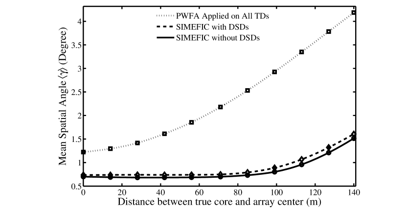
Figure 7: Mean value of angle between the EAS primary direction and the direction which has been found by SIMEFIC algorithm assuming the array with non DSDs (solid curve), SIMEFIC algorithm assuming the array with DSDs (dashed curve) and by PWFA applied on all TDs (dotted curve) versus the distance of the true core from array center.

References

- [1] J.G. Gonzalez, Phys. Rev. D 74 (2006) 027701.
- [2] K. Greisen, Annu. Rev. Nucl. Sci 10 (1960) 63.
- [3] M. Nagano, Nucl. J. Phys. G 10 (1984) 1295.
- [4] J. Linsley, J. Phys. G 12 (1986) 51.
- [5] P. Bassi, et al., Phys. Rev. 92 (1953) 441.
- [6] G. Agnetta et al., Astropart. Phys. 6 (1997) 301.
- [7] M. Ambrosio et al., Astropart. Phys. 11 (1999) 473.
- [8] D. Heck et al.,Report FZKA6019 (Forschungszentrum Karlsruhe (1998).
- [9] A. Fasso et al., Computing in High Energy and Nuclear Physics 2003 Conference (CHEP2003)(arXiv:hep-ph/0306267).
- [10] A. Ferrari et al., CERN-2005-10 (2005), INFN/TC 05/11, SLAC-R-773.
- [11] S.S. Ostapchenko, Nucl. Phys. B (Proc. Suppl.) QGSJET-II 151 (2006) 143.
- [12] S.S. Ostapchenko, Phys. Rev. D, 74 (2006) 014026.
- [13] H. Fesefeldt, Report PITHA-85/02 (1985)