A gauge-technique Ansatz for the three gluon vertex of the background field method

Abstract:

The vertex connecting one background gluon with two quantum ones constitutes a central ingredient in the gauge-invariant Schwinger-Dyson equation that determines the non-perturbative dynamics of the gluon propagator. This vertex satisfies a Ward identity with respect to the background gluon, and a Slavnov-Taylor identity with respect to the two quantum gluons. We present a complete Ansatz for this vertex, which satisfies both aforementioned identities. This entire construction depends crucially on a set of constraints relating the various form-factors of the ghost Green’s functions appearing in the Slavnov-Taylor identity satisfied by the vertex. The validity of these constraints is demonstrated to all orders.

1 Introduction

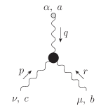
Figure 1: The $BQQ$ three-gluon vertex. The background leg is indicated by the gray circle.

The three-gluon vertex describing the interaction of one background ($B$) and two quantum ($Q$) gluons (“$BQQ$ vertex”, for short) [see Fig. 1] is of particular interest, because it constitutes a key ingredient for understanding certain important aspects of non-perturbative QCD.

As has been explained in a series of recent articles [1], the fully dressed version of the $BQQ$ vertex is instrumental for the gauge-invariant truncation the Schwinger-Dyson equations (SDE) obtained within the general formalism based on the Pinch Technique (PT) [2] and the Background Field Method (BFM) [3], and especially for the crucial transversality properties displayed by the SDE governing the gluon self-energy. In particular, and contrary to what happens in the conventional formulation, the “one-loop dressed” subset of (only gluonic!) diagrams, (corresponding to the first step in the aforementioned SDE truncation), furnishes an exactly transverse gluon self-energy.

The SDEs of the PT-BFM have been particularly successful in reproducing recent lattice data [4, 5], which clearly indicate that the gluon propagator and the ghost dressing function of Yang-Mills in the Landau gauge are infrared finite both in $SU(2)$ [6, 7] and in $SU(3)$. The non-perturbative form of the $BQQ$ vertex is essential for accomplishing this task. Indeed, the way the gluon acquires a dynamically generated (momentum-dependent) mass (first paper in [2]), which, in turn, accounts for the infrared finiteness of the aforementioned Green’s functions, is determined by a subtle interplay between various crucial features of this special vertex [8].

To be sure, the non-perturbative behavior of the $BQQ$ vertex is determined by its own SDE equation, which contains the various multiparticle kernels appearing in the “skeleton expansion”. However, for practical purposes, one is forced to resort to an Ansatz for this vertex, obtained through the so-called “gauge-technique” [9].

The idea behind the gauge-technique is fairly simple, especially in an abelian context: one constructs an expression for the unknown vertex out of the ingredients appearing in the Ward identity (WI) it satisfies. These ingredients must be put together in a way such that the resulting expression satisfies the WI automatically. The most typical example of such a construction is found in the case of the three-particle vertex of scalar QED, describing the interaction of a photon with a pair of charged scalars. This vertex, to be denoted by $\bm{\Gamma}_{\mu}$, satisfies the abelian all-order WI

$$q^{\mu}\bm{\Gamma}_{\mu}={\mathcal{D}}^{-1}(k+q)-{\mathcal{D}}^{-1}(k)\,,$$ (1)

where ${\mathcal{D}}(k)$ is the fully-dressed propagator of the scalar field. Thus, in this case, the gauge-technique Ansatz for $\Gamma_{\mu}$, obtained by Ball and Chiu [10], after “solving” the above WI, under the additional requirement of not introducing kinematic singularities, is

$$\bm{\Gamma}_{\mu}=\frac{(2k+q)_{\mu}}{(k+q)^{2}-k^{2}}\left[{\mathcal{D}}^{-1}(k+q)-{\mathcal{D}}^{-1}(k)\right],$$ (2)

which clearly satisfies Eq. (1).

Returning to the case at hand, and according to the philosophy explained above, one must construct the $BQQ$ vertex out of the ingredients appearing in the WI and Slavnov-Taylor identity (STI) it satisfies (third paper in [1]), and in such a way that these identities are automatically satisfied. This is a complicated task, because some of the ingredients appearing in the STI (i.e., the Green’s functions originating from the ghost sector) are themselves constrained by yet another set of (largely unexplored) WIs and STIs, which must be exactly preserved, or else the entire construction will collapse, or major complications will appear in subsequent steps of the SDE treatment.

The purpose of this talk is to describe in some detail how the longitudinal part of the $BQQ$ vertex can be obtained by “solving” the corresponding WI and STI, and the important role played by the constraints relating the various ghost Green’s functions appearing in the STI. A complete account of the important implications of this construction on the SDE of the gluon propagator will be given elsewhere [11].

2 The $BQQ$ vertex and its basic properties

The $BQQ$ vertex constitutes without a doubt one of the most fundamental ingredients of the PT, making its appearance already at the basic level of the one-loop construction. Specifically, defining the tree-level conventional three-gluon vertex through the expression (all momenta entering)

$$i\Gamma^{(0)}_{A^{a}_{\alpha}A^{b}_{\mu}A^{c}_{\nu}}(q,r,p) = gf^{abc}\Gamma^{(0)}_{\alpha\mu\nu}(q,r,p)$$

$$\Gamma^{(0)}_{\alpha\mu\nu}(q,r,p) = g_{\mu\nu}(r-p)_{\alpha}+g_{\alpha\nu}(p-q)_{\mu}+g_{\alpha\mu}(q-r)_{\nu},$$ (3)

the diagrammatic rearrangements giving rise to the PT Green’s functions (propagators and vertices) stem exclusively from the characteristic decomposition [2]

$$\Gamma^{(0)}_{\alpha\mu\nu}(q,r,p) = \widetilde{\Gamma}^{(0)}_{\alpha\mu\nu}(q,r,p)+(1/\xi)\Gamma^{{\rm P}}_{\alpha\mu\nu}(q,r,p),$$

$$\widetilde{\Gamma}^{(0)}_{\alpha\mu\nu}(q,r,p) = g_{\mu\nu}(r-p)_{\alpha}+g_{\alpha\nu}(p-q+r/\xi)_{\mu}+g_{\alpha\mu}(q-r-p/\xi)_{\nu},$$

$$\Gamma^{{\rm P}}_{\alpha\mu\nu}(q,r,p) = g_{\alpha\mu}p_{\nu}-g_{\alpha\nu}r_{\mu}.$$ (4)

In the equations above, $\xi$ represents the gauge fixing parameter that appears also in the definition of the (full) gluon propagator $\Delta^{ab}_{\mu\nu}(q)=\delta^{ab}\Delta_{\mu\nu}(q)$, with

$$i\Delta_{\mu\nu}(q)=-i\left[P_{\mu\nu}(q)\Delta(q^{2})+\xi\frac{q_{\mu}q_{\nu}}{q^{4}}\right];\qquad\Delta^{-1}_{\mu\nu}(q)=i\left[P_{\mu\nu}(q)\Delta^{-1}(q^{2})+\xi q_{\mu}q_{\nu}\right]$$ (5)

and $P_{\mu\nu}(q)=g_{\mu\nu}-q_{\mu}q_{\nu}/q^{2}$ the dimensionless transverse projector. The scalar co-factor $\Delta(q^{2})$ is related to the all-order gluon self-energy $\Pi_{\mu\nu}(q)=P_{\mu\nu}(q)\Pi(q^{2})$ through

$$\Delta^{-1}({q^{2}})=q^{2}+i\Pi(q^{2})\equiv q^{2}J(q^{2}),$$ (6)

where the quantity $J(q^{2})$ is defined in order to maintain a notational proximity with [12].

Note that the PT makes no ab initio reference to a background gluon; at the level of the Yang-Mills Lagrangian there is only one gauge field, $A$, which is quantized in the usual way, by means of a linear gauge-fixing term of the type $\frac{1}{2\xi}(\partial_{\mu}A^{\mu})^{2}$ (the $R_{\xi}$ gauges). However, the decomposition (4) assigns right from the start a special role to the leg carrying the momentum $q$, that is to be eventually identified with the background leg. Thus, unlike $\Gamma^{(0)}_{\alpha\mu\nu}(q,r,p)$, which is Bose-symmetric with respect to all its three legs, the vertex $\widetilde{\Gamma}^{(0)}$ is in fact Bose-symmetric only with respect to the (quantum) $\mu$ and $\nu$ legs. In addition, it satisfies the simple Ward identity

$$iq^{\alpha}\widetilde{\Gamma}^{(0)}_{\alpha\mu\nu}(q,r,p)=\Delta^{-1}_{0\,\,\mu\nu}(p)-\Delta^{-1}_{0\,\,\mu\nu}(r)\,,$$ (7)

where $\Delta_{0}^{\mu\nu}(q)$ is the tree-level version of the $\Delta^{\mu\nu}(q)$ given in Eq. (5). In higher orders, the $BQQ$ vertex is constructed through the systematic triggering of internal STIs in the diagrams of the conventional (higher order) three-gluon vertex (see the tree last items in  [2]).

On the other hand, when quantizing the theory within the BFM [3], the $BQQ$ vertex $\Gamma_{\widehat{A}AA}$ arises directly, as a consequence of the splitting of the classical gauge field into a background and a quantum component, $A\to A+\widehat{A}$. In addition, one introduces a special gauge-fixing function that is linear in the quantum field $A$, and preserves gauge invariance with respect to the background field $\widehat{A}$ (the corresponding gauge-fixing parameter is denoted $\xi_{Q}$). Let us denote the full $BQQ$ vertex by $\Gamma_{\widehat{A}^{a}_{\alpha}A^{b}_{\mu}A^{c}_{\nu}}(q,r,p)$, and factor out the usual coupling and color structure,

$$i\Gamma_{\widehat{A}^{a}_{\alpha}A^{b}_{\mu}A^{c}_{\nu}}(q,r,p)=gf^{abc}\widetilde{\Gamma}_{\alpha\mu\nu}(q,r,p)\,.$$ (8)

At tree-level, $\widetilde{\Gamma}_{\alpha\mu\nu}\to\widetilde{\Gamma}^{(0)}_{\alpha\mu\nu}(\xi\to\xi_{Q})$, i.e. it is given by the expression for $\widetilde{\Gamma}^{(0)}_{\alpha\mu\nu}$ in Eq. (4), after the simple replacement $\xi\to\xi_{Q}$.

In order to cast the upcoming WI and STIs into a more compact form, it is convenient to consider instead of $\widetilde{\Gamma}_{\alpha\mu\nu}(q,r,p)$ the minimally modified vertex

$$\widetilde{\bm{\Gamma}}_{\alpha\mu\nu}(q,r,p)=\widetilde{\Gamma}_{\alpha\mu\nu}(q,r,p)+(1/\xi_{Q})\Gamma^{{\rm P}}_{\alpha\mu\nu}(q,r,p)\,.$$ (9)

Evidently, $\widetilde{\bm{\Gamma}}_{\alpha\mu\nu}(q,r,p)$ and $\widetilde{\Gamma}_{\alpha\mu\nu}(q,r,p)$ differ only at tree level; specifically, using Eq. (4), we see immediately that

$$\widetilde{\bm{\Gamma}}_{\alpha\mu\nu}^{(0)}(q,r,p)^{(0)}=\Gamma^{(0)}_{\alpha\mu\nu}(q,r,p).$$ (10)

Incidentally, notice that $\widetilde{\bm{\Gamma}}_{\alpha\mu\nu}(q,r,p)$ coincides with the vertex appearing in the SDE for the gluon propagator, when projecting to the Landau gauge [4].

Thus, $\widetilde{\bm{\Gamma}}$ satisfies a (ghost-free) WI when contracted with the momentum $q_{\alpha}$ of the background gluon, while it satisfies a STI when contracted with the momentum of the quantum gluons ($r_{\mu}$ or $p_{\nu}$). They are given by (second item in [1])

$$q^{\alpha}\widetilde{\bm{\Gamma}}_{\alpha\mu\nu}(q,r,p) = p^{2}J(p^{2})P_{\mu\nu}(p)-r^{2}J(r^{2})P_{\mu\nu}(r)$$

$$r^{\mu}\widetilde{\bm{\Gamma}}_{\alpha\mu\nu}(q,r,p) = F(r^{2})\left[q^{2}\widetilde{J}(q^{2})P_{\alpha}^{\mu}(q)H_{\mu\nu}(q,r,p)-p^{2}J(p^{2})P_{\nu}^{\mu}(p)\widetilde{H}_{\mu\alpha}(p,r,q)\right]$$

$$p^{\nu}\widetilde{\bm{\Gamma}}_{\alpha\mu\nu}(q,r,p) = F(p^{2})\left[r^{2}J(r^{2})P_{\mu}^{\nu}(r)\widetilde{H}_{\nu\alpha}(r,p,q)-q^{2}\widetilde{J}(q^{2})P_{\alpha}^{\nu}(q)H_{\nu\mu}(q,p,r)\right].$$ (11)

In the above equations, $F(q^{2})$ is the ghost dressing function, related to the ghost propagator $D(q^{2})$ through

$$iD^{ab}(q^{2})=i\delta^{ab}\frac{F(q^{2})}{q^{2}},$$ (12)

while the propagator $\widetilde{\Delta}$ is related to the conventional one, $\Delta(q^{2})$, through the so-called “background quantum identity” [13]

$$\Delta(q^{2})=\left[1+G(q^{2})\right]\widetilde{\Delta}(q^{2}).$$ (13)

The function $G$ appearing above is the $g_{\mu\nu}$ co-factor in the Lorentz decomposition of the auxiliary function $\Lambda_{\mu\nu}(q)$ defined through

$$\Lambda_{\mu\nu}(q) = \int_{k}\!\Delta_{\mu}^{\sigma}(k)D(q-k)H_{\nu\sigma}(-q,q-k,k)$$ (14)

$$= g_{\mu\nu}G(q^{2})+\frac{q_{\mu}q_{\nu}}{q^{2}}L(q^{2}),$$

and shown in Fig. 2, together with the definitions and conventions of the functions $H$ and $\widetilde{H}$. Therefore, requiring the vertex Ansatz to satisfy the STIs above implies that in its expression certain combinations of the ghost auxiliary functions $G$, $H$ and $\widetilde{H}$ will also appear.

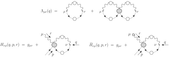
Figure 2: Definitions and conventions of the auxiliary functions $\Lambda$, $H$ and $\widetilde{H}$. The color and coupling dependence for the combination shown, $c^{a}(q)A_{\mu}^{b}(r)A_{\nu}^{*c}(p)$, is $gf^{acb}$. White blobs represent connected Green’s functions, while gray blobs denote the two-gluon–two-ghost kernel. Note that the kernel is one-particle irreducible with respect to perpendicular cuts.

3 Identities of the ghost sector

In this section we explain the field-theoretic origin of a set of constraints whose validity must be invoked when attempting to solve the WI and STI of Eq. (11), in order to construct the $BQQ$ vertex. As we will shortly, the underlying reason for having to resort to these constraints is the fact that the resulting system has more equations than unknowns, a fact known from the early work of Ball and Chiu [12] on the conventional three-gluon vertex.

To begin with, we observe that, since both the $R_{\xi}$ and the BFM are linear gauge fixing conditions, there exists a constraint coming from the equation of motion of the Nakanishi-Lautrup fields (the so called ghost or Faddeev-Popov equation), which, in turn, implies that the functions $H$ and $\widetilde{H}$ are related to the corresponding gluon-ghost trilinear vertices $\Gamma_{\alpha}$ and $\widetilde{\Gamma}_{\alpha}$. In particular one has (second item in [1])

$$p^{\nu}H_{\nu\alpha}(p,r,q)+\Gamma_{\alpha}(r,q,p) = 0$$

$$p^{\nu}\widetilde{H}_{\nu\alpha}(p,r,q)+\widetilde{\Gamma}_{\alpha}(r,q,p) = r_{\alpha}F^{-1}(r^{2}),$$ (15)

where at tree-level

$$\Gamma^{(0)}_{\alpha}(r,q,p)=-p_{\alpha};\qquad\widetilde{\Gamma}^{(0)}_{\alpha}(r,q,p)=(r-p)_{\alpha}.$$ (16)

In addition, while the function $\widetilde{H}$ satisfies the WI

$$q^{\alpha}\widetilde{H}_{\nu\alpha}(p,r,q)=-p_{\nu}F^{-1}(p^{2})-r_{\nu}F^{-1}(r^{2}),$$ (17)

the function $H$ fulfills the STI

$$q^{\alpha}H_{\nu\alpha}(p,r,q)=-F^{-1}(q^{2})\left[p_{\nu}F^{-1}(p^{2})C(q,r,p)+r^{\alpha}F^{-1}(r^{2})H_{\nu\alpha}(p,q,r)\right],$$ (18)

where $C$ represents yet another ghost auxiliary function $\Gamma_{ccc^{*}}$ involving two ghosts and an anti-ghost field (with momentum $p$). To proceed further, we decompose $H$ and $\widetilde{H}$ in terms of their basic tensor forms

$$H_{\nu\alpha}(p,r,q) = g_{\alpha\nu}a_{qrp}-r_{\alpha}q_{\nu}b_{qrp}+q_{\alpha}p_{\nu}c_{qrp}+q_{\nu}p_{\alpha}d_{qrp}+p_{\alpha}p_{\nu}e_{qrp},$$

$$\widetilde{H}_{\nu\alpha}(p,r,q) = g_{\alpha\nu}\widetilde{a}_{qrp}-r_{\alpha}q_{\nu}\widetilde{b}_{qrp}+q_{\alpha}p_{\nu}\widetilde{c}_{qrp}+q_{\nu}p_{\alpha}\widetilde{d}_{qrp}+p_{\alpha}p_{\nu}\widetilde{e}_{qrp}.$$ (19)

where, following the notation of [12] we have introduced the short-hand $a_{qrp}$ for $a(q,r,p)$, and similarly for all other form factors appearing in (19). Then, one can use the identities (17) and (18) in order to constrain certain combinations of these form factors. Indeed, from the WI (17) one finds

$$\widetilde{a}_{qrp}-(q\cdot r)\widetilde{b}_{qrp}+(q\cdot p)\widetilde{d}_{qrp} = F^{-1}(r^{2})$$

$$q^{2}\widetilde{c}_{qrp}+(q\cdot p)\widetilde{e}_{qrp}+F^{-1}(p^{2}) = F^{-1}(r^{2}),$$ (20)

while the STI (18) gives

$$F(r^{2})\left[a_{qrp}-(q\cdot r)b_{qrp}+(q\cdot p)d_{qrp}\right] = F(q^{2})\left[a_{rqp}-(q\cdot r)b_{rqp}+(p\cdot r)d_{rqp}\right]$$

$$F^{-1}(q^{2})\left[q^{2}c_{qrp}+(q\cdot p)e_{qrp}\right]+F^{-1}(p^{2})C_{prq} = F^{-1}(r^{2})\left[a_{rqp}-(q\cdot r)b_{rqp}+(p\cdot r)d_{rqp}\right]$$ (21)

$$- F^{-1}(r^{2})\left[r^{2}c_{rqp}+(p\cdot r)e_{rqp}\right],$$

where, according to our conventions, $C_{prq}=C(q,r,p)$.

Incidentally, notice that the first equation in (21), together with its cyclic permutations of momenta and indices, represent the three constraints found in [12] [viz. Eq. (2.10) in that article] as necessary conditions to determine the conventional three-gluon vertex from solving the corresponding STIs (the system is in fact overconstrained displaying more equations than unknowns); indeed we see from the above that such constraints are a consequence of the STI satisfied by the $H$ function (in [12] these constraints were explicitly verified at the one-loop level only).

Finally, let us conclude by observing that $H$ and $\widetilde{H}$ are related by the BQI

$$\widetilde{H}_{\nu\alpha}(p,r,q) = \left[g_{\alpha}^{\gamma}+\Lambda_{\alpha}^{\gamma}(q)\right]H_{\nu\alpha}(p,r,q)-r^{\gamma}F^{-1}(r^{2})N_{\alpha\gamma\nu}(q,r,p)$$ (22)

$$+ p_{\nu}F^{-1}(p)O_{\alpha}(q,r,p),$$

where the auxiliary functions $N$ and $O$ are related to certain auxiliary functions involving the background source $\Omega$, namely $\Gamma_{\Omega AA^{*}}$ and $\Gamma_{\Omega cc^{*}}$.

4 Solving the Ward and Slavnov-Taylor identities

In what follows we determine an Ansatz for $\widetilde{\bm{\Gamma}}$ by solving the WI and STIs given in Eq. 11. It is well-known that the gauge technique, in general, can only furnish information about the longitudinal part of any vertex, leaving its transverse (automatically conserved) part completely undetermined. This fact, in turn, is known to be of limited importance in the infrared (in the presence of a mass gap!), but is essential for the multiplicative renormalizability of the resulting SDEs. For the purposes of this work, we will ignore such refinements, settling for subtractive renormalizability only.

Therefore, following [12], the 14 possible tensorial structures necessary for describing a general three-gluon vertex are separated into two groups, 10 of them spanning the longitudinal part of the vertex, and the remaining 4 the (totally) transverse part; then only the former group is considered.

Specifically, in the basis of [12] the longitudinal part of $\widetilde{\bm{\Gamma}}_{\alpha\mu\nu}(q,r,p)$ has the form

$$\widetilde{\bm{\Gamma}}^{(\ell)}_{\alpha\mu\nu}(q,r,p)=\sum_{i=1}^{10}X_{i}(q,r,p)\ell^{i}_{\alpha\mu\nu}(q,r,p),$$ (23)

with the explicit form of the tensors $\ell^{i}$ given by

$$\ell^{1}_{\alpha\mu\nu}=(q-r)_{\nu}g_{\alpha\mu}$$

.

(24)

Notice that excluding $\ell^{10}$, each of the remaining $\ell^{i+3}$ can be obtained by the corresponding $\ell^{i}$ through cyclic permutation of momenta and indices; in addition, Bose symmetry with respect to the quantum legs requires that $\Gamma$ change sign under the interchange of the corresponding Lorentz indices and momenta, thus implying the relations

$$X_{1}(q,p,r)=X_{7}(q,r,p)$$

(25)

The form factors $X_{i}$ are then fully determined by solving the system of linear equations generated by the identities given in Eq. (11). The procedure is conceptually straightforward, but operationally rather cumbersome. One first substitutes on the lhs of Eq. (11) the general tensorial decomposition of $\widetilde{\bm{\Gamma}}^{(\ell)}_{\alpha\mu\nu}(q,r,p)$ given in Eq. (23), and then equates the coefficients of the resulting tensorial structures to those appearing on the rhs. Thus, one obtains a system of equations expressing the form factors $X_{i}(q,p,r)$ in terms of combinations of quantities such as $J$, $F$, etc.

In what follows we will only report the set of independent equations, i.e., we will omit equations that can be obtained from existing ones by implementing the change $p\leftrightarrow r$ and using the constraints of  (25). Thus, for example, the equation $X_{7}+X_{8}+(q\cdot r)X_{10}=J(p)$ does not form part of the set of independent equations, because it can be obtained from the second equation in Eq.(26) below, by carrying out the aforementioned transformation, and using the corresponding relations from Eq. (25).

Thus, from the abelian WI one obtains the following 4 equations

$$(p^{2}-r^{2})X_{4}-q^{2}X_{5}-(r\cdot p)(p^{2}-r^{2})X_{6} = p^{2}J(p)-r^{2}J(r)$$

$$X_{1}-X_{2}-(q\cdot p)X_{10} = J(r)$$

$$X_{1}+X_{2}-X_{7}+X_{8} = 0$$

$$2X_{1}+(p^{2}-r^{2})X_{6}-2X_{7}+q^{2}X_{10} = 0,$$ (26)

where the form of the second equation has been simplified by making use of the third.

Similarly, from the non-abelian STI one obtains 5 equations, namely

$$(r^{2}-q^{2})X_{1}-p^{2}X_{2}-(q\cdot r)(r^{2}-q^{2})X_{3} = F(p)\left[{\widetilde{a}}_{qpr}r^{2}J(r)-a_{rpq}q^{2}{\widetilde{J}}(q)\right]$$

$$(r^{2}-q^{2})X_{3}-2X_{4}+2X_{7}+p^{2}X_{10} = F(p)\left[({\widetilde{b}}_{qpr}+{\widetilde{d}}_{qpr})r^{2}J(r)-(b_{rpq}+d_{rpq})q^{2}{\widetilde{J}}(q)\right]$$

$$-X_{7}+X_{8}+(r\cdot p)X_{10} = F(p)\left\{(r\cdot p){\widetilde{b}}_{qpr}J(r)-\left[a_{rpq}+(q\cdot r){d}_{rpq}\right]{\widetilde{J}}(q)\right\}$$

$$X_{4}+X_{5}+(q\cdot p)X_{10} = F(p)\left\{\left[{\widetilde{a}}_{qpr}+(q\cdot r){\widetilde{d}}_{qpr}\right]J(r)-(q\cdot p)b_{rpq}{\widetilde{J}}(q)\right\}$$

$$-X_{4}+X_{5}+X_{7}+X_{8} = (q\cdot r)F(p)\left[-{\widetilde{b}}_{qpr}J(r)+b_{rpq}{\widetilde{J}}(q)\right].$$ (27)

Clearly, there are 5 additional equations, obtained from the second STI; however, they too can be obtained from the set of equations (27) by imposing the transformation $r\leftrightarrow p$ and using the relations given in Eq. (25), and are therefore omitted.

As anticipated, we have more equations than form factors [remember the constraints of Eq. (25)!], and therefore the appearance of a set of non-trivial constraints for the ghost sector. It turns out that these constraints are precisely those furnished by Eq. (20) and the first relation of Eq. (21). Therefore the system can be solved, and one finds a solution of the type presented in [12] with a modified ghost-sector, reading

$$X_{1}(q,r,p) = \frac{1}{4}{\widetilde{J}}(q)\left\{-p^{2}b_{prq}F(r)+[2a_{rpq}+p^{2}b_{rpq}+2(q\cdot r)d_{rpq}]F(p)\right\}$$

$$+ \frac{1}{4}J(r)\left[2+(r^{2}-q^{2}){\widetilde{b}}_{qpr}F(p)\right]+\frac{1}{4}J(p)\,p^{2}\,{\widetilde{b}}_{qrp}F(r)$$

$$X_{2}(q,r,p) = \frac{1}{4}{\widetilde{J}}(q)\left\{(q^{2}-r^{2})b_{prq}F(r)+[2a_{rpq}+(r^{2}-q^{2})b_{rpq}+2(q\cdot r)d_{rpq}]F(p)\right\}$$

$$+ \frac{1}{4}J(r)\left[-2+p^{2}{\widetilde{b}}_{qpr}F(p)\right]+\frac{1}{4}J(p)\,(r^{2}-q^{2})\,{\widetilde{b}}_{qrp}F(r)$$

$$X_{3}(q,r,p) = \frac{F(p)}{q^{2}-r^{2}}\left\{{\widetilde{J}}(q)\left[a_{rpq}-(q\cdot p)d_{rpq}\right]-J(r)\left[{\widetilde{a}}_{qpr}-(r\cdot p){\widetilde{d}}_{qpr}\right]\right\}$$

$$X_{4}(q,r,p) = \frac{1}{4}{\widetilde{J}}(q)q^{2}\left[b_{prq}F(r)+b_{rpq}F(p)\right]+\frac{1}{4}J(r)\left[2-q^{2}{\widetilde{b}}_{qpr}F(p)\right]$$

$$+ \frac{1}{4}J(p)\left[2-q^{2}{\widetilde{b}}_{qrp}F(r)\right]$$

$$X_{5}(q,r,p) = \frac{1}{4}{\widetilde{J}}(q)(p^{2}-r^{2})\left[b_{prq}F(r)+b_{rpq}F(p)\right]+\frac{1}{4}J(r)\left[2+(r^{2}-p^{2}){\widetilde{b}}_{qpr}F(p)\right]$$

$$- \frac{1}{4}J(p)\left[2+(p^{2}-r^{2}){\widetilde{b}}_{qrp}F(r)\right]$$

$$X_{6}(q,r,p) = \frac{J(r)-J(p)}{r^{2}-p^{2}}$$

$$X_{7}(q,r,p) = X_{1}(q,p,r)$$

$$X_{8}(q,r,p) = -X_{2}(q,p,r)$$

$$X_{9}(q,r,p) = X_{3}(q,p,r)$$

$$X_{10}(q,r,p) = \frac{1}{2}\left\{{\widetilde{J}}(q)\left[b_{prq}F(r)-b_{rpq}F(p)\right]+J(r)F(p){\widetilde{b}}_{qpr}-J(p)F(r){\widetilde{b}}_{qrp}\right\}.$$ (28)

5 Conclusions

We have presented a complete Ansatz for the $BQQ$ three-gluon vertex, which is in absolute conformity with both the WI and the STI given in Eq. (11). An important step in this construction is the formal, all-order derivation of the crucial constraints relating the various form factors of the ghost Green’s function, involved in the STI of Eq. (11), an indispensable step for realizing this construction.

It is important to emphasize that the Ansatz for the $BQQ$ vertex presented here is valid for any value of the gauge-fixing parameter used to quantize the theory. Indeed, even though the various ingredients appearing in the solution Eq. (28), such as $J$, $F$, etc, depend explicitly on $\xi$ (or on $\xi_{Q}$), the precise functional dependence of the form factors $X_{i}$ on $J$, $F$, etc, given in Eq. (28), is valid for any $\xi$, given that it originates from the solution of the WI and STI of Eq. (11), whose form is $\xi$-independent.

This last point is particularly important given the existing perspectives [14] of carrying out large-volume lattice simulations in covariant gauges other than the Landau gauge ($\xi\neq 0$). In particular, the possibility of simulating propagators in the background gauges (especially the background Feynman gauge, $\xi_{Q}=1$) opens up the exiting possibility of studying central objects of the PT on the lattice [15].

An additional important point, not addressed here, is related to the way the $BQQ$ vertex triggers the Schwinger mechanism [16], which, in turn, is responsible for the dynamical generation of a gluon mass. As is well-known [17], the relevant three-gluon vertex (in this case the $BQQ$ vertex ) must contain longitudinally coupled massless poles, in order for gauge invariance to be preserved. We emphasize that the Ansatz presented here does not incorporate such poles, which must be supplied at a subsequent step. We hope to accomplish this task in the near future.

Acknowledgments:

I thank the organizers of this Workshop for their warm hospitality and stimulating environment. This research was supported by the European FEDER and Spanish MICINN under grant FPA2008-02878, and the Fundación General of the UV.

References

[1]
A. C. Aguilar and J. Papavassiliou,
JHEP 0612, 012 (2006);
D. Binosi and J. Papavassiliou,
Phys. Rev. D 77(R), 061702 (2008);
JHEP 0811, 063 (2008).
[2]
J. M. Cornwall,
Phys. Rev. D 26, 1453 (1982);
J. M. Cornwall and J. Papavassiliou,
Phys. Rev. D 40, 3474 (1989);
D. Binosi and J. Papavassiliou,
Phys. Rev. D 66(R), 111901 (2002);
J. Phys. G 30, 203 (2004);
Phys. Rept. 479, 1-152 (2009).
[3]
See, e.g., L. F. Abbott,
Nucl. Phys. B 185, 189 (1981), and references therein.
[4]
A. C. Aguilar, D. Binosi and J. Papavassiliou,
Phys. Rev. D 78, 025010 (2008).
[5]
J. Rodriguez-Quintero,
PoS LC2010, 023 (2010);
arXiv:1012.0448 [hep-ph].
[6]
A. Cucchieri and T. Mendes,
PoS LAT2007, 297 (2007);
Phys. Rev. Lett. 100, 241601 (2008);
Phys. Rev. D 81, 016005 (2010);
PoS LATTICE2010, 280 (2010);
arXiv:1101.4779 [hep-lat].
[7]
I. L. Bogolubsky, E. M. Ilgenfritz, M. Muller-Preussker and A. Sternbeck,
PoS LATTICE, 290 (2007);
Phys. Lett. B 676, 69 (2009);
O. Oliveira and P. J. Silva,
PoS LAT2009, 226 (2009);
P. O. Bowman et al.,
Phys. Rev. D 76, 094505 (2007).
[8]
A. C. Aguilar, J. Papavassiliou,
Phys. Rev. D81, 034003 (2010).
[9]
A. Salam,
Phys. Rev. 130, 1287 (1963);
A. Salam and R. Delbourgo,
Phys. Rev. 135, B1398 (1964);
R. Delbourgo and P. C. West,
J. Phys. A 10, 1049 (1977);
Phys. Lett. B 72, 96 (1977).
[10]
J. S. Ball and T. W. Chiu,
Phys. Rev. D 22, 2542 (1980).
[11]
D. Binosi and J. Papavassiliou,
arXiv:1102.5662 [hep-ph].
[12]
J. S. Ball and T. W. Chiu,
Phys. Rev. D 22, 2550 (1980)
[Erratum-ibid. D 23, 3085 (1981)].
[13]
P. A. Grassi, T. Hurth and M. Steinhauser,
Annals Phys. 288, 197 (2001);
D. Binosi and J. Papavassiliou,
Phys. Rev. D 66, 025024 (2002).
[14]
A. Cucchieri, T. Mendes and E. M. S. Santos,
Phys. Rev. Lett. 103, 141602 (2009);
arXiv:1101.5080 [hep-lat].
[15]
A. Cucchieri, T. Mendes, G. M. Nakamura and E. M. S. Santos,
arXiv:1102.5233 [hep-lat].
[16]
J. S. Schwinger,
Phys. Rev. 125, 397 (1962);
Phys. Rev. 128, 2425 (1962).
[17]
R. Jackiw and K. Johnson,
Phys. Rev. D 8, 2386 (1973);
J. M. Cornwall and R. E. Norton,
Phys. Rev. D 8 (1973) 3338;
E. Eichten and F. Feinberg,
Phys. Rev. D 10, 3254 (1974).