A Bayesian parameter estimation approach to pulsar time-of-arrival analysis

Abstract

The increasing sensitivities of pulsar timing arrays to ultra-low frequency (nHz) gravitational waves promises to achieve direct gravitational wave detection within the next 5-10 years. While there are many parallel efforts being made in the improvement of telescope sensitivity, the detection of stable millisecond pulsars and the improvement of the timing software, there are reasons to believe that the methods used to accurately determine the time-of-arrival (TOA) of pulses from radio pulsars can be improved upon. More specifically, the determination of the uncertainties on these TOAs, which strongly affect the ability to detect GWs through pulsar timing, may be unreliable. We propose two Bayesian methods for the generation of pulsar TOAs starting from pulsar “search-mode” data and pre-folded data. These methods are applied to simulated toy-model examples and in this initial work we focus on the issue of uncertainties in the folding period. The final results of our analysis are expressed in the form of posterior probability distributions on the signal parameters (including the TOA) from a single observation.

1 Introduction

Pulsar timing arrays could well be used to detect ultra-low frequency gravitational waves (GWs) within the next 5-10 years [1]. This is an especially exciting prospect given the concurrent efforts of the LIGO-Virgo Scientific collaboration (LVC) whose aim is to make direct detection of GWs (in the $\sim$10-1000 Hz regime) using the 2^nd generation of ground based interferometric detectors within the same timescale [2].

In this work we outline the beginnings of a Bayesian approach to the detection of GWs with pulsar timing using simplistic signal and noise models onto which can be built further levels of sophistication in the future. A key long-term aim of our analysis is to improve our ability to time existing millisecond pulsars by a factor of 3-10 [3, 4]. One of the main problems to be overcome is to be able to sensibly account for the excess low-frequency noise seen in many stable millisecond pulsars [5]. We focus on a single piece of the complete pulsar timing analysis, the generation of time-of-arrival (TOA) measurements. Given a single pulsar observation, this is the arrival time of the average pulse at the telescope where in this context “average” means the sum of pulses produced by “folding” the data with a periodicity equal to the assumed pulse period. It is from these TOAs that pulsar astronomers then model the spin evolution of pulsars taking into account the motion of the radio telescope relative to the pulsar [6]. The presence of GWs in the field between the telescope and the pulsar will result in small shifts in the arrival times of pulses [7, 8].

We choose to limit our investigation to single pulsar observations (typically $100-1000$s seconds in duration) and since TOAs are defined in the reference frame of the telescope and the GW timescale $\gg$ the timescale of a single observation, we are able to neglect any GW effect in our analysis. We will discuss two different strategies for the estimation of parameters (including the TOA) from two separate starting points, what we will call “search-mode” data and “pre-folded” data. In both cases we perform the analysis using a commonly used Bayesian integration algorithm in order to obtain posterior probability distributions on the signal parameters.

We note that our approach is aimed as a starting point for future more realistic scenarios and that it can be viewed as an approach being built from the bottom-up. We mean this in the sense that we try to start from the most basic datasets available (see Secs. 3 and 4) and attempt to build a data-analysis framework in which the multitude of physical processes affecting pulsar signals can be included and accounted for. In contrast, other work on the specifics of GW detection using pulsar timing arrays has taken a more top-down approach. These analyses have started with timing residuals, the result of a fit to the data assuming non GW effects (effectively the end of the pulsar data processing chain), and either neglected this potential inconsistency [9, 10] or made attempts to account for it [11].

The paper is organised as follows. In Sec. 2 we describe our simplistic signal and noise model. In Secs. 3 and 4 we then go on to describe the form of this signal model in two different representations of the original dataset. The basic concepts concerning our Bayesian approach to the parameter estimation problem can be found in Sec. 5 and finally we discuss our conclusions and potential future developments in Sec. 6.

2 The signal : A toy model

We begin with a dataset defined on a discrete 2-dimensional grid of time $t_{j}$ versus radio-frequency $f_{k}$ of which an example is shown in Fig. 1. Data of this kind is often referred to as “search-mode” data since this data format is the kind used when performing searches for unknown pulsars. Each of the $M$ rows of the 2-dimensional grid is a timeseries of radio-frequency power measured within a radio-frequency band with central frequency $f_{k}$. Typical sampling times and observation durations are $\sim 10$s of $\mu$seconds and $100-1000$s of seconds respectively. Typical frequency channel widths and total detector bandwidths are $\sim 1$ MHz and $100-1000$s MHz respectively. For “search-mode” data we assume the following signal model

$$x(t_{j},f_{k})=s(t_{j},f_{k})+n(t_{j},f_{k}),$$ (1)

where $x(t_{j},f_{k})$ represents the discretely sampled dataset, $s(t_{j},f_{k})$ is the signal and $n(t_{j},f_{k})$ is the noise which for simplicity we assume as independent Gaussian distributed random variables with zero mean. The signal itself we define as

$$s(t_{j},f_{k})=\sum_{\alpha=0}^{n^{\prime}-1}A\exp\left[-\frac{\left(t_{j}-\mu_{\alpha k}\right)^{2}}{2w^{2}}\right],$$ (2)

where $\alpha$ sums over all $n^{\prime}$ pulses that intersect with the observation. We use $A$ as the pulse peak amplitude, $w$ as the pulse width, and $\mu_{\alpha k}$ as the centre of the $\alpha$’th pulse in the $k$’th frequency channel. Note that we are modelling each pulse as having a single Gaussian profile component and that the amplitude and width remain constant in both time and with frequency channel. The inclusion of additional Gaussian pulse components requires only a trivial modification to the model. In Sec. 6 we discuss numerous potential additions and modifications required to make this toy model a more accurate representation of a real pulsar signal.

The time at the centre of each pulse is defined as

$$\mu_{\alpha k}=\left(\phi_{k}+\alpha\right)P+\xi_{\alpha},$$ (3)

where $P$ is the constant pulse period and $\phi_{k}$ is the phase (defined on the range $\left[0,1\right)$) of the first pulse in the observation for the $k$’th frequency channel. We have also included a random pulse “jitter” term where for each pulse we apply a random shift to the pulse arrival time where each shift $\xi_{\alpha}$ is drawn from a Gaussian distribution with zero mean and variance $\sigma_{\xi}^{2}$. Such effects have been observed in several pulsars and can be attributed to unknown processes in the pulse emission mechanism and possibly related to giant pulses [12, 13, 14, 15, 16]. We show in Sec. 3 that for our purposes, the effect of this particular pulse “jitter” modelling can be absorbed into a subset of the other signal parameters.

The phase of the first pulse in each frequency channel $\phi_{k}$ can be related to the phase $\Phi_{0}$, defined as the phase of the pulse at the midpoint frequency channel $f_{\mathrm{mid}}=(f_{M}-f_{1})/2$ and with reference to the midpoint of the observation $t=T/2$ by

$$\phi_{k}=\mathrm{mod}\left(\frac{T}{2P}+\frac{\Delta t(f_{k})}{P}+\Phi_{0},1\right).$$ (4)

The relative delay due to dispersion in the $k$’th frequency channel $\Delta t(f_{k})$ is given by

$$\Delta t(f_{k})=4.148808\times 10^{3}\left(f_{k}^{-2}-f_{\mathrm{mid}}^{-2}\right)DM\,\,\,\mathrm{sec},$$ (5)

where $DM$ is the dispersion measure in $\mathrm{cm}^{-3}\mathrm{pc}$ and the units of the frequencies are MHz. Note that in our simplistic model we do not account for dispersion smearing within individual channels.

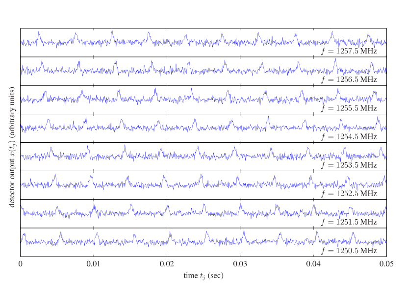
Figure 1: A example of time vs frequency channel “search-mode” data showing a portion of a simulated dataset consisting of a strong signal in Gaussian noise. Here we show only the first $0.05$ seconds of data ($\Delta t=64\,\mu$sec) for $8$ $1$-MHz wide frequency channels. The signal has an amplitude $A=5$, pulse width $w=0.25$ msec, period $P=5$ msec, a phase $\Phi_{0}=0.2$, and a dispersion measure $DM=100\,\mathrm{cm}^{-3}\mathrm{pc}$. The noise has unit variance.

3 Using “search-mode” data in the Fourier domain

The signals received from pulsars are periodic and their frequency evolution is slow i.e. the timescale of frequency variation $\gg$ the pulse period. By Fourier transforming each channel’s time-series we find that a pulsar signal can be represented as a series of narrow-band harmonics as shown in Fig. 2. In a realistic situation we would expect to have some prior knowledge of the pulsar frequency before performing an analysis and therefore transforming the data in such a way allows us to isolate the regions in the dataset where the signal is concentrated (at the harmonics). This in-turn allows us to be economic with the data samples that we are interested in and will make any numerical likelihood computation more efficient. Let us define the discrete Fourier transform as

$$\tilde{x}(\nu_{l})=\sum_{j=0}^{N-1}x(t_{j})e^{-2\pi jl/N}\Delta t,$$ (6)

where $\nu_{l}$ represents the elements of a vector containing the positive discrete Fourier frequencies with frequency spacing $1/T$ and where $N$ is the number of time samples. When applied to the time series from each frequency channel of a noise-free signal (defined by Eqs. 2,3) we obtain

$$\tilde{s}(\nu_{l},f_{k}) = \sum_{j=0}^{N-1}\sum_{\alpha=0}^{n^{\prime}-1}A\exp\left[-\frac{\left(t_{j}-\mu_{\alpha k}\right)^{2}}{2w^{2}}\right]e^{-2\pi jl/N}\Delta t,$$ (7)

$$= \sum_{\alpha=0}^{n^{\prime}-1}\tilde{s}_{\alpha}(\nu_{l},f_{k}),$$

where we have decomposed the complete Fourier transform into the Fourier transform of each pulse. We then have

$$\tilde{s}_{\alpha}(\nu_{l},f_{k}) = A\sum_{j=0}^{N-1}\exp\left[-\frac{\left(t_{j}-\mu_{\alpha k}\right)^{2}}{2w^{2}}-2\pi jl/N\right]\Delta t,$$ (8)

$$\approx A\exp\left\{-2\pi i\nu_{l}\mu_{\alpha k}\right\}\int_{-\infty}^{\infty}\exp\left\{\frac{y^{2}}{2w^{2}}-2\pi i\nu_{l}y\right\}\,dy,$$

$$= Aw\sqrt{2\pi}\exp\left\{-2\pi i\nu_{l}\mu_{\alpha k}-2\pi^{2}w^{2}\nu_{l}^{2}\right\},$$

where we have approximated the discrete sum over time samples with the continuous integral over the dummy variable $y=t-\mu_{\alpha k}$ assuming that each pulse itself spans $\gg 1$ time bin and is not truncated by the edges of the timeseries. We can now perform the sum over $\alpha$ (the individual pulses) to obtain the complete Fourier transform. However, note that $\mu_{\alpha k}$ is a function of $\xi_{\alpha}$, the random individual pulse arrival time jitter. We choose to average over this random variable under the assumption that there are a large number of pulses within the observation time. This averaging procedure leads to the following replacement:

$$e^{-2\pi i\nu_{l}\xi}\rightarrow\Large\langle e^{-2\pi i\nu_{l}\xi}\Large\rangle = \int_{-\infty}^{\infty}\frac{e^{-\xi^{2}/2\sigma_{\xi}^{2}}}{\sqrt{2\pi\sigma^{2}_{\xi}}}\,e^{-2\pi i\nu_{l}\xi}\,d\xi,$$ (9)

$$= e^{-2\pi^{2}\nu_{l}^{2}\sigma_{\xi}^{2}},$$

where we have replaced the pulse jitter term with its expectation value and used a Gaussian distribution for the pulse jitter with a zero mean and variance of $\sigma^{2}_{\xi}$. Finally we obtain the following expression for the Fourier transform of the signal only timeseries

$$\tilde{s}(\nu_{l},f_{k})=\frac{A_{\xi}w_{\xi}T}{P}\sqrt{2\pi}\exp\left\{-2\pi^{2}\nu_{l}^{2}w_{\xi}^{2}\right\}\exp\left\{-2\pi i\phi_{k}\nu_{l}\right\}\tilde{W}_{l}.$$ (10)

We can see from this equation that in the Fourier domain the signal can be decomposed into four parts. There is a real positive amplitude term proportional to the pulse amplitude, width, and number of pulses ($n\approx T/P$) which is multiplied by a frequency dependent envelope function that decays with increasing frequency at a rate proportional to the pulse width. There is also a unit amplitude complex phase term dependent upon the initial phase of the pulse in the given frequency channel multiplied by a second complex phase term $\tilde{W}_{l}$ given by

$$\tilde{W}_{l}=\frac{P}{T}\exp\left\{2\pi i\nu_{l}P\right\}\left[\frac{1-\exp\left\{-2\pi i\nu_{l}T\right\}}{\exp\left\{2\pi i\nu_{l}P\right\}-1}\right],$$ (11)

which, in the limit of $T\gg P$ can be written as

$$\tilde{W}_{l}=\sum_{\beta=0}^{n}\left\{\frac{\sin(2\pi\Delta\nu_{l\beta}T)}{2\pi\Delta\nu_{l\beta}T}+i\left[\frac{\cos(2\pi\Delta\nu_{l\beta}T)-1}{2\pi\Delta\nu_{l\beta}T}\right]\right\},$$ (12)

where $\Delta\nu_{l\beta}=\nu_{l}-\beta/P$ and $\beta$ labels the individual signal harmonics of which there are $n$. This final complex phase term contains the information regarding the location and phase of the signal harmonics. We can now see that each signal harmonic is identical in shape but will each have a different phase and amplitude. In addition, as one moves to different frequency channels the phase of a given harmonic will be rotated by a quantity dependent upon the dispersion measure.

Note that we have also re-parameterised the pulse amplitude and width using

$$A_{\xi} = \frac{Aw}{\sqrt{w^{2}+\sigma_{\xi}^{2}}},$$ (13)

$$w_{\xi} = \sqrt{w^{2}+\sigma_{\xi}^{2}},$$ (14)

since with the addition of pulse jitter there exists a degeneracy between the original pulse amplitude and width. The product of the amplitude and width determine the overall amplitude of the Fourier transform of the signal and the sum of the squares of the width and the pulse jitter parameter determine the rate of the reduction in amplitude of the harmonics with increasing frequency. Using the data to measure this amplitude and its attenuation with increasing frequency will therefore not allow us to constrain all three parameters.

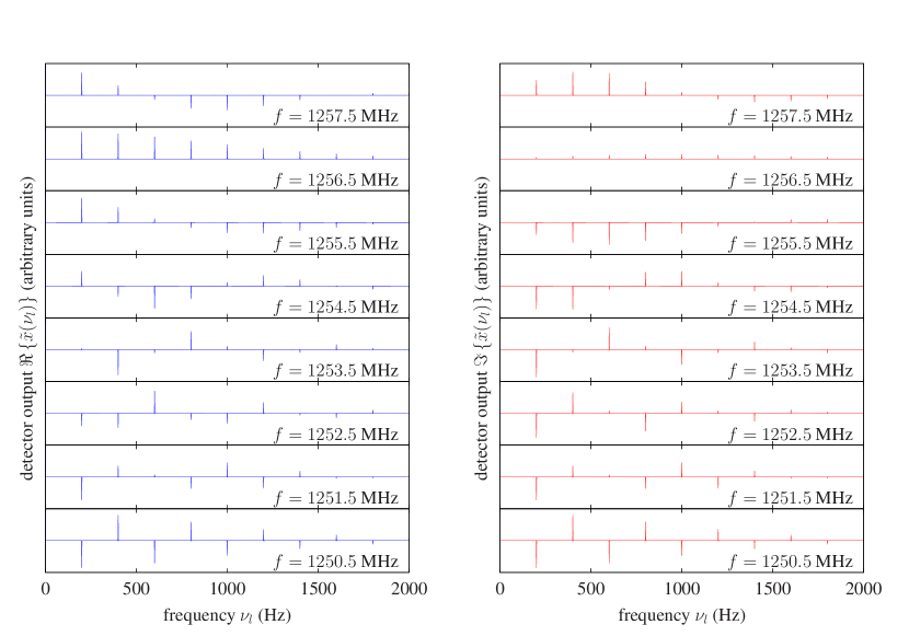
Figure 2: A example of Fourier transformed “search-mode” data showing a portion of a simulated dataset consisting of a strong signal in Gaussian noise. The panels on the left show (in blue) the real part of the complex Fourier transform of the data as a function of Fourier frequency for $8$ $1$-MHz wide frequency channels. The imaginary parts are shown (in red) on the right. The dataset used to generate this plot is identical to that shown in Fig. 1 and we have truncated the frequency range at $2$ kHz since there the harmonic content of the signal is significantly reduced beyond this frequency.

4 Using folded data

The majority of pulsar timing data is pre-processed and reduced in volume by the process of folding. In this process, sections of the time series from each frequency channel of an observation will be folded with an assumed pulse period. At the time of folding this pulse period will not necessarily be the most accurate value. The pulse period itself is updated and refined with each subsequent observation. However, once data have been folded, most notably for older observations, the original search mode data may be lost, meaning that re-folding with the more refined period is not possible.

We will focus on the effect of folding with an inaccurate pulse period. One can argue that since the most basic initial pulse period estimates will require a coherent measurement over some prior observation spanning many pulses, we should expect an initial worst case fractional uncertainty in the pulse period of $\sim P/T$ which for a $10$ msec pulsar period and a $100$ second coherent observation equates to a period error of $\sim 1$ $\mu$second. In addition to the pulse period, for realistic analyses a number of other parameters are used in the folding procedure such as the sky position coordinates, the intrinsic pulsar spin-frequency derivatives, the dispersion measure plus orbital parameters if the source is in a binary system. In our toy model we ignore these complications.

We choose to define the result of the folding process for a single observation as a 2-dimensional grid of pulse profiles labelled by time and channel frequency, an example of which is shown in Fig. 3. To perform a consistent analysis of such a dataset we take into account the fact that profiles have been obtained using a non-precise value of the pulse period. If we consider a dataset that has already been folded at a specific (non-exact) pulse period $P^{\prime}=P+\Delta P$ then we can define a new folded dataset as

$$X(\phi^{\prime},P^{\prime},f_{k})=\sum_{\beta=0}^{n-1}x\Big{(}(\beta+\phi^{\prime})P^{\prime},f_{k}\Big{)},$$ (15)

where $\beta$ indexes each fold up to $n=\mathrm{floor}(T/P^{\prime})$. Substituting in our signal model (Eqs. 2 and 3) we can accurately approximate the discretely summed noise-free pulse profile as

$$S(\phi^{\prime},P^{\prime},f_{k}) \approx \frac{A_{\xi}w_{\xi}}{|\Delta P|}\sqrt{\frac{\pi}{2}}\sum_{z=-1}^{1}\left[\mathrm{erf}\left(a_{z}+b\right)-\mathrm{erf}\left(a_{z}\right)\right],$$ (16)

where we have used

$$a_{z} = \frac{|\Delta P|}{\Delta P}\,\left[\frac{(P+\Delta P)(\phi^{\prime}+z)-\phi_{k}P}{w_{\xi}\sqrt{2}}\right],$$ (17)

$$b = \frac{|\Delta P|(n-1)}{w_{\xi}\sqrt{2}}.$$ (18)

In the calculation of Eq. 16 we have again replaced the pulse arrival time jitter term with its expectation value (as done in Sec. 3) and approximated the sum over pulses with a continuous integral. We have also been forced to re-parameterise the pulse amplitude and width parameters for the same reasons as described in the previous section and have chosen to use an identical re-parameterisation (defined in Eqs. 13 and 14). The summation over the index $z$ is simply to account for the fact that folding a signal with an arbitrary initial phase may separate the pulse profile into significant contributions spanning the $\phi^{\prime}=0=1$ point. This also acts to account for the fact that if folding with an incorrect pulse period the true pulse will slowly drift across the $\phi^{\prime}$ space. In this scenario the tails of neighbouring pulses begin to contribute to the sum and by including the $z=\pm 1$ terms we are accurately modelling this effect.

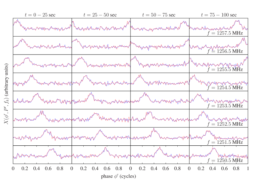
Figure 3: An example simulated folded dataset showing folded pulse profiles for $4$ sub-intervals each spanning $25$ seconds and for $8$ frequency channels each spanning $1$ MHz. The simulated signal parameters are equal to those defined and used in Figs. 1 and 2 with the exception that here the signal amplitude $A=0.1$ is significantly lower. Two curves are plotted in each panel, the blue curves are profiles obtained through folding with the true pulse period $P$. The red curves are the profiles obtained through folding with an pulse period error $\Delta P^{\prime}=10$ nsec. Note that this size period error is equivalent to a phase error of $\sim 0.01$ cycles over the course of a sub-integration.

5 A Bayesian analysis

The Bayesian component to our approach can be viewed as standard in the sense that we aim to simply apply Bayes probability theorem to the time-of-arrival problem with the intention of computing marginalised posterior probability distributions on the signal parameters.

Bayes theorem can be expressed as

$$p(\boldsymbol{\theta}|\boldsymbol{x},\mathcal{M})=\frac{L(\boldsymbol{x}|\boldsymbol{\theta},\mathcal{M})\pi(\boldsymbol{\theta}|\mathcal{M})}{E(\mathcal{M}|\boldsymbol{x})},$$ (19)

where the term on the left-hand-side is the joint posterior probability distribution on the parameter set $\boldsymbol{\theta}$ given a dataset defined by the vector $\boldsymbol{x}$ and a chosen model represented by $\mathcal{M}$. The function $L(\boldsymbol{x}|\boldsymbol{\theta},\mathcal{M})$ is the likelihood function describing the dataset $\boldsymbol{x}$ given the parameter set $\boldsymbol{\theta}$ and the model $\mathcal{M}$. The function $\pi(\boldsymbol{\theta}|\mathcal{M})$ is the joint prior probability distribution on the parameter set $\boldsymbol{\theta}$ given the model $\mathcal{M}$. Finally we have the Bayesian evidence $E(\mathcal{M}|\boldsymbol{x},\boldsymbol{\theta})$ representing the probability of the model $\mathcal{M}$ given the dataset $\boldsymbol{x}$.

To obtain marginalised posterior distributions on a particular signal parameter we are required to perform a multi-dimensional integration of the joint posterior distribution over the remaining parameters. Formally this can be written as

$$p(\theta_{m}|\boldsymbol{x},\mathcal{M})\propto\int_{\mathcal{S}}d^{n}\boldsymbol{\theta^{\prime}}\,L(\boldsymbol{x}|\boldsymbol{\theta},\mathcal{M})\pi(\boldsymbol{\theta}|\mathcal{M}),$$ (20)

where the parameter vector $\boldsymbol{\theta^{\prime}}$ consists of the subset of parameters in the vector $\boldsymbol{\theta}$ excluding the parameter $\theta_{m}$ and where $\mathcal{S}$ defines the volume of integration on that space. Note that there is no dependence upon the Bayesian evidence in the calculation of the marginalised posterior distribution since it is independent of the parameter values themselves and can be absorbed into the normalisation of the posterior distribution.

In practice the calculation of posterior distribution functions can be a difficult and computationally intensive procedure. Over the last decade much work has been dedicated to the efficient numerical computation of posterior probability distributions and more recently to the evaluation of the Bayesian evidence. One of the now standard tools available for Bayesian data analysis is the Markov-Chain-Monte-Carlo (MCMC) [17, 18], an efficient method for obtaining random samples drawn from a posterior probability distribution of which there are a number of variations [19, 20, 21, 22, 23, 24]. More recently the strategy known as “nested sampling” [25, 26] has given the data analyst the ability to accurately estimate the Bayesian evidence, a model dependent quantity used to perform model selection. The first direct application of this strategy was to perform cosmological model selection using WMAP data [27]. For this work we chose to perform our analysis using the freely available nested sampling algorithm MultiNest [28]. Note that this algorithm has been specifically designed to be robust with respect to multi-modal posterior distributions and to compute the Bayesian evidence. For this work we use it purely to obtain posterior probability distributions on the pulsar parameters.

Let us now define the likelihood functions specific to the two approaches described in Secs. 3 and 4. The likelihood function for the Fourier domain approach to the “search-mode” data is defined as

$$L^{\mathrm{sm}}(\boldsymbol{\tilde{x}}|\boldsymbol{\theta})=\left(2\pi\sigma_{f}^{2}\right)^{-NM/4}\exp\left\{-\frac{1}{2\sigma^{2}_{f}}\sum_{j=0}^{N/2-1}\sum_{k=0}^{M-1}|\tilde{x}_{jk}-\tilde{s}_{jk}(\boldsymbol{\theta})|^{2}\right\},$$ (21)

where $N/2$ and $M$ are the total number of Fourier-frequency and radio-frequency bins respectively and we define $\boldsymbol{\theta}=\{A_{\xi},w_{\xi},DM,P,\Phi_{0}\}$ as the vector of signal parameters. We have used $\sigma_{f}^{2}$ to represent the frequency domain noise variance which we assume to be Gaussian, white, and stationary and therefore constant for all Fourier and radio frequency bins. In this ideal scenario the frequency domain noise variance is related to the time domain noise variance $\sigma_{t}^{2}$ by $\sigma_{f}^{2}=N(\Delta t)^{2}\sigma_{t}^{2}$.

The likelihood function for the folded data can similarly be written as

$$L^{\mathrm{fold}}(\boldsymbol{X}|\boldsymbol{\theta})=\left(2\pi\sigma_{X}^{2}\right)^{-N_{\mathrm{s}}M/2}\exp\left\{-\frac{1}{2\sigma^{2}_{X}}\sum_{j=0}^{N_{\mathrm{s}}-1}\sum_{k=0}^{M-1}\left(X_{jk}-S_{jk}(\boldsymbol{\theta})\right)^{2}\right\},$$ (22)

where $N_{s}$ is the number of equal length sub-intervals into which each frequency channel’s timeseries has been divided. The noise contribution in a particular folded phase bin is simply the sum of $n=\mathrm{floor}(T/P^{\prime})$ Gaussian distributed variables of variance $\sigma_{t}^{2}$ and hence $\sigma_{X}^{2}=n\sigma_{t}^{2}$. The parameter vector $\boldsymbol{\theta}$ is identical to that defined for the search-mode data.

In general the choice of prior probability distribution functions on the parameters $\boldsymbol{\theta}$ would be chosen according to one’s prior beliefs on the values of those parameters. However, for the purposes of our toy model investigation we choose “flat” prior distributions for all parameters with prior ranges chosen to be far greater than the expected span of the posterior distributions. In this case we do not favour any particular choice of parameter values over any others.We note that in making this choice we are disregarding a powerful feature of the Bayesian analysis, the ability to correctly incorporate prior information into the result. However, one can show that for strong signal-to-noise ratios the effect of the prior on the posterior is dominated by that of the likelihood function itself.

To conclude this section we would like to make it clear that what we have described in Secs. 3 and 4 do not constitute two separate models. We have described two separate representations of the same original dataset and have in-fact used the same signal model. Model selection therefore could not be applied to these two methods. Our aim is to compare the effectiveness of each choice of dataset representation by contrasting the posterior distributions on the signal parameters when a single common time-radio-frequency dataset is used to generate both the Fourier-radio-frequency and a folded dataset. Model selection using the Bayesian evidence and the computation of the Bayes factor (the ratio of model evidences) and odds-ratio (the Bayes factor multiplied by the ratio of prior model probabilities) is a potentially powerful tool in future advanced implementations of our analysis strategy. Our choice of nested sampling implementation, MultiNest, has been designed specifically to compute the Bayesian evidence, making model selection between different pulsar signal models an obvious and easy to implement extension of our approach.

6 Discussion

Shown in Fig. 4 is an example of typical marginalised posterior probability distributions on the signal parameters $\boldsymbol{\theta}=\{A_{\xi},w_{\xi},DM,P,\Phi_{0}\}$ plus the time-of-arrival parameter $t_{\mathrm{TOA}}$. The latter is not independent of the other parameters and is a function of both the phase parameter and the pulse period such that $t_{\mathrm{TOA}}=\Phi_{0}P$ and is therefore defined as the arrival time of the first pulse received at the mid-point frequency channel immediately following the mid-point of the observation.

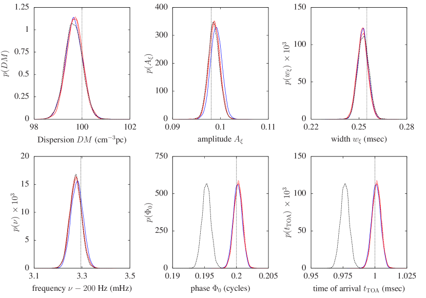
Figure 4: The marginalised posterior distributions on the signal parameters for a simulated signal in Gaussian noise. In solid blue we show the results obtained when using the Fourier domain representation of the “search-mode” data. In solid red we show the results obtained when using folded data as the input for the case where the data was folded with the true pulse period. In dashed red we show the results for the folding scenario where an incorrect period, $\Delta P=10$ nanoseconds, has been used to fold the data and we have accounted for this within the signal model. The dashed black curves show the result where this effect has not been accounted for. The vertical dotted black lines indicate the values of the true signal parameters. For all results the data was converted into the Fourier and folded representations from a single common time-frequency dataset of length $100$ sec with sampling time $64$ $\mu$sec and frequency range of $8$ MHz consisting of $8$ channels each of $1$ MHz bandwidth.

Our results show that the ability to determine the signal parameters is unaffected by the choice of data representation when comparing the Fourier domain approach and the folded data. This is apparent from the consistent widths of the posterior distributions which define the uncertainty in parameter estimation. The clear effect that we see is the discrepancy between the location of the posterior distributions for the case where the error in folding period has been accounted for and where it has not. We see that the estimation of the dispersion, pulse amplitude, pulse width, and pulse frequency is only marginally affected. However, the phase parameter and therefore the time-of-arrival estimate, is strongly biased by the false assumption that the signal has been folded with the correct pulse period. For the results shown in Fig. 4 the pulse period error of $10$ nsecs is equivalent to an accumulated phase error of only $3.6$ degrees over the length of the $25$ sec sub-integrations. This appears as a $\sim 1.8$ degree ($\equiv 0.005$ cycles) error in the estimate of $\Phi_{0}$ leading to a $\sim 25$ $\mu$second error in the estimate of the time-of-arrival value.

It is clear that the work presented here is intended only as a potential starting point for more advanced applications of Bayesian data analysis techniques to the problem of pulsar timing. A clear difference between our approach as described here and established techniques is that we have obtained our pulsar parameter estimates from a single simulated observation. The standard approach is to employ a more global strategy in which the process of producing a time-of-arrival measurement for a given observation is not just a function of the given observation but of all existing observations of the pulsar. Each TOA represents the reduction of an entire observation into a single number after having performed a global fit (over all observations) for a set of common pulsar parameters e.g. pulse period, the period derivatives, the sky position, proper motion, pulse shape parameters, the dispersion measure, etc. When new observations are taken, the procedure is repeated and these parameters are refined. As discussed in Sec. 4, as data is recorded it is often reduced (in terms of data volume) by folding at an assumed pulse period and in addition may be partially de-dispersed with an assumed dispersion measure. The detrimental effect of this process (as seen in our results) will rapidly diminish as more and more observations are made but further analysis is required to rule out such effects as contributors to the low-frequency timing noise seen in the msec pulsars.

The scope of this work is limited to the generation of TOAs but we would also like to briefly discuss the specific aim of gravitational wave detection using pulsar timing arrays. From a purely theoretical Bayesian data analysis perspective in an ideal scenario, firstly, one would use an un-reduced dataset spanning all observations of all relevant pulsars. Secondly one would construct a model including all pulsar signal parameters and all gravitational wave signal parameters. After applying sensible prior distributions to all of these parameters one would compute marginalised posterior distributions on both pulsar and gravitational wave parameters and perform model selection. We could then establish whether the observations coupled with our prior beliefs were consistent with the presence of gravitational waves. In practice this is a very difficult task for various reasons but most notably due to the vast computational resources required to process the vast volume of un-reduced data and to explore the multi-dimensional parameter space describing the entire pulsar array and the intervening gravitational wave. For this reason, in terms of gravitational wave detection, constructing a reduced dataset is highly desirable. In fact, the problem of gravitational wave detection using timing residuals (the difference between the time-of-arrival values and those attained by fitting a gravitational wave free pulsar model) as the initial dataset have already been applied to the specific case of searching for the gravitational wave stochastic background [11, 10].

The apparent separation of the complete gravitational wave detection problem into a gravitational wave free component, from which a reduced dataset is produced, and then a second component in which this reduced dataset is then analysed including the effects of gravitational waves, seems potentially problematic. Under the assumption that each TOA measurement is independent of all others one can argue strongly that the effect of a low-frequency gravitational wave on each measurement is negligible and that the TOA truly represents the unambiguous arrival time of an average pulse within that observation and defined at some epoch. As soon as one performs a global fit (neglecting gravitational waves) over all observations of a given pulsar a gravitational wave of sufficient amplitude will affect the best fit pulsar parameters. Such a procedure could absorb some fraction of a gravitational wave into the pulsar parameter estimates (e.g the pulsar period derivatives). In future work we hope to address this issue and to provide a comparison between an analysis using independent TOA measurements as a dataset for gravitational wave detection and an analysis using globally estimated TOAs.

In addition we hope to be able to include, and account for, many of the physical effects and data analysis issues that we have ignored in our toy model approach. These include a more robust treatment of the noise where we allow time and frequency variation and investigate the validity of the assumption of Gaussianity. In reference to this we hope to also include the effects of radio frequency interference (RFI) and investigate methods in which we are able to analytically marginalise over the noise and therefore potentially avoid the need to estimate it. We also aim to include the effect of polarisation into the analysis. A search-mode dataset is itself the product of two independent radio signal polarisation measurements which are combined as a function of the Stokes parameters. These parameters can be incorporated into the Bayesian framework and uncertainties on these parameters can be marginalised over in parallel with the signal parameters. Less well defined effects to consider include a time and frequency varying pulse profile parameterisation, time varying dispersion measure, scattering, scintillation and nulling. Finally, we hope to develop this work beyond the toy model to a point at which it can be applied to real pulsar data. In such a scenario we will also have to incorporate barycentric routines [6] to include the obvious effects of detector motion, sky position uncertainty and, where applicable, binary orbital motion.

References

References

- [1] G. Hobbs. Pulsar timing array projects. In IAU Symposium, volume 261 of IAU Symposium, pages 228–233, January 2010.
- [2] The LIGO Scientific Collaboration. LIGO: the Laser Interferometer Gravitational-Wave Observatory. Reports on Progress in Physics, 72(7):076901–+, July 2009.
- [3] F. Jenet, L. S. Finn, J. Lazio, A. Lommen, M. McLaughlin, I. Stairs, D. Stinebring, J. Verbiest, A. Archibald, Z. Arzoumanian, D. Backer, J. Cordes, P. Demorest, R. Ferdman, P. Freire, M. Gonzalez, V. Kaspi, V. Kondratiev, D. Lorimer, R. Lynch, D. Nice, S. Ransom, R. Shannon, and X. Siemens. The North American Nanohertz Observatory for Gravitational Waves. ArXiv e-prints, September 2009.
- [4] G. Hobbs, A. Lyne, and M. Kramer. Pulsar Timing Noise. Chinese Journal of Astronomy and Astrophysics Supplement, 6(2):020000–175, December 2006.
- [5] G. Hobbs, A. Archibald, Z. Arzoumanian, D. Backer, M. Bailes, N. D. R. Bhat, M. Burgay, S. Burke-Spolaor, D. Champion, I. Cognard, W. Coles, J. Cordes, P. Demorest, G. Desvignes, R. D. Ferdman, L. Finn, P. Freire, M. Gonzalez, J. Hessels, A. Hotan, G. Janssen, F. Jenet, A. Jessner, C. Jordan, V. Kaspi, M. Kramer, V. Kondratiev, J. Lazio, K. Lazaridis, K. J. Lee, Y. Levin, A. Lommen, D. Lorimer, R. Lynch, A. Lyne, R. Manchester, M. McLaughlin, D. Nice, S. Oslowski, M. Pilia, A. Possenti, M. Purver, S. Ransom, J. Reynolds, S. Sanidas, J. Sarkissian, A. Sesana, R. Shannon, X. Siemens, I. Stairs, B. Stappers, D. Stinebring, G. Theureau, R. van Haasteren, W. van Straten, J. P. W. Verbiest, D. R. B. Yardley, and X. P. You. The International Pulsar Timing Array project: using pulsars as a gravitational wave detector. Classical and Quantum Gravity, 27(8):084013–+, April 2010.
- [6] G. B. Hobbs, R. T. Edwards, and R. N. Manchester. TEMPO2, a new pulsar-timing package - I. An overview. MNRAS, 369:655–672, June 2006.
- [7] S. Detweiler. Pulsar timing measurements and the search for gravitational waves. apj, 234:1100–1104, December 1979.
- [8] R. W. Hellings and G. S. Downs. Upper limits on the isotropic gravitational radiation background from pulsar timing analysis. apjl, 265:L39–L42, February 1983.
- [9] F. A. Jenet, A. Lommen, S. L. Larson, and L. Wen. Constraining the Properties of Supermassive Black Hole Systems Using Pulsar Timing: Application to 3C 66B. apj, 606:799–803, May 2004.
- [10] M. Anholm, S. Ballmer, J. D. E. Creighton, L. R. Price, and X. Siemens. Optimal strategies for gravitational wave stochastic background searches in pulsar timing data. prd, 79(8):084030–+, April 2009.
- [11] R. van Haasteren, Y. Levin, P. McDonald, and T. Lu. On measuring the gravitational-wave background using Pulsar Timing Arrays. mnras, 395:1005–1014, May 2009.
- [12] A. Kinkhabwala and S. E. Thorsett. Multifrequency Observations of Giant Radio Pulses from the Millisecond Pulsar B1937+21. apj, 535:365–372, May 2000.
- [13] M. Kramer, S. Johnston, and W. van Straten. High-resolution single-pulse studies of the Vela pulsar. mnras, 334:523–532, August 2002.
- [14] I. Cognard, J. A. Shrauner, J. H. Taylor, and S. E. Thorsett. Giant Radio Pulses from a Millisecond Pulsar. apj, 457:L81+, February 1996.
- [15] V. I. Kondratiev, M. V. Popov, V. A. Soglasnov, Y. Y. Kovalev, N. Bartel, W. Cannon, and A. Y. Novikov. Probing cosmic plasma with giant radio pulses. Astronomical and Astrophysical Transactions, 26:585–595, December 2007.
- [16] A. D. Kuzmin and A. A. Ershov. Detection of giant radio pulses from the pulsar PSR B0656+14. Astronomy Letters, 32:583–587, September 2006.
- [17] W. R. Gilks, S. Richardson, and D. J. Spiegelhalter. Markov chain Monte Carlo in practice. Chapman & Hall / CRC, Boca Raton, 1996.
-
[18]
A. Gelman, J. B. Carlin, H. S. Stern, and D. B. Rubin.
Bayesian Data Analysis.
Chapman & Hall, London, 1995 (ISBN 0-412-03991-5).
Gelman et al. summarize the full breadth of Bayesian analysis. A strong point of this presentation is its thoughtful and informative style, and avoidance of detailed mathematical derivations. - [19] Enzo Marinari and Giorgio Parisi. Simulated tempering: A new monte carlo scheme. EUROPHYS.LETT., 19:451, 1992.
- [20] Robert Gramacy, Richard Samworth, and Ruth King. Importance tempering. Statistics and Computing, 20:1–7, January 2010.
- [21] Bo Cai, Renate Meyer, and François Perron. Metropolis—hastings algorithms with adaptive proposals. Statistics and Computing, 18:421–433, December 2008.
- [22] Antonietta Mira. On metropolis-hastings algorithms with delayed rejection. Metron - International Journal of Statistics, 0(3-4):231–241, 2001.
- [23] Sergio Hernandez-Marin, Andrew M. Wallace, and Gavin J. Gibson. Bayesian analysis of lidar signals with multiple returns. IEEE Trans. Pattern Anal. Mach. Intell., 29:2170–2180, December 2007.
- [24] M. Trias, A. Vecchio, and J. Veitch. Delayed rejection schemes for efficient Markov-Chain Monte-Carlo sampling of multimodal distributions. ArXiv e-prints, April 2009.
- [25] John Skilling. Nested sampling. volume 735, pages 395–405. AIP, 2004.
-
[26]
D. S. Sivia.
Data Analysis: A Bayesian Tutorial.
Clarendon (Oxford Univ. Press), Oxford, 1996 (ISBN: 0-19-851762-9 or
0-19-851889-7 in paperback).
Divinder Sivia presents a very straightforward account of Bayesian analysis. Rather than going for mathematical rigor and an axiomatic approach, he introduces concepts as they are needed to solve a sequence of increasingly complex analysis problems. Very readable and informative. - [27] P. Mukherjee, D. Parkinson, and A. R. Liddle. A Nested Sampling Algorithm for Cosmological Model Selection. apjl, 638:L51–L54, February 2006.
- [28] F. Feroz and M. P. Hobson. Multimodal nested sampling: an efficient and robust alternative to Markov Chain Monte Carlo methods for astronomical data analyses. mnras, 384:449–463, February 2008.