Pegging Numbers for Various Tree Graphs
Abstract.
In the game of pegging, each vertex of a graph is considered a hole into which a peg can be placed. A pegging move is performed by jumping one peg over another peg, and then removing the peg that has been jumped over from the graph. We define the pegging number as the smallest number of pegs needed to reach all the vertices in a graph no matter what the distribution. Similarly, the optimal-pegging number of a graph is defined as the smallest distribution of pegs for which all the vertices in the graph can be reached. We obtain tight bounds on the pegging numbers and optimal-pegging numbers of complete binary trees and compute the optimal-pegging numbers of complete infinitary trees. As a result of these computations, we deduce that there is a tree whose optimal-pegging number is strictly increased by removing a leaf. We also compute the optimal-pegging number of caterpillar graphs and the tightest upper bound on the optimal-pegging numbers of lobster graphs.
1. Introduction
One of the better known peg solitaire games is described by Berlekamp, Conway, and Guy in their book, Winning Ways for Your Mathematical Plays [1]. In this game we are presented with an infinite square grid on a Cartesian plane. At each intersection there is a hole in which a peg can be placed, and all the holes in the lower half-plane are filled. We can move pegs on the grid in the following manner: if we have two adjacent pegs, one of which is adjacent to an empty hole, then the peg further from the hole can jump over the peg next to the hole and fill it. The peg that was jumped over is then removed from the grid. As it turns out, the farthest up the grid we can get using only legal pegging moves is a distance of 4 holes.
A graph version of this game, where in place of a grid we have any graph where each vertex represents a hole that can be filled by a peg, was studied by Helleloid, Khalid, Matchett-Wood, and Moulton in [2] and later by Wood in [4]. This game is a variation of the graph game pebbling [3], where each move removes 2 pebbles from a vertex and places one of the pebbles on an adjacent vertex. A pegging move on a graph consists of removing two pegs from adjacent vertices and placing one peg on a unfilled vertex adjacent to one of the first two holes. Given some initial distribution of pegs on a graph, we say we can reach a vertex if after a (possibly empty) series of pegging moves we can cover it with a peg. Research on pegging mainly involves finding the optimal-pegging number, the size of the smallest distribution which can reach all the vertices in a graph, and finding the pegging number, the smallest number of pegs needed to reach all the vertices in a graph no matter what the distribution. These terms are modeled after the definitions of optimal-pebbling numbers and pebbling numbers, respectively. In their paper, Helleloid et al. study the pegging and optimal-pegging numbers of various types of graphs including paths, cycles, hypercubes, and complete graphs. They also explore basic pegging properties of graphs with diameters of at most 3. Wood examines various graph products and the effects of small variations of distributions of pegs on their reach.
This paper explores the pegging properties of various types of tree graphs. In Section 2, we provide background and terminology pertaining to the pegging of general graphs. In Section 3 we present pegging properties of general trees. In Section 4, we find tight bounds on the pegging and optimal-pegging numbers of the complete binary tree. In Section 5, we define the concept of an infinitary tree, and find the optimal-pegging number of this tree, which follows the Fibonacci sequence. As a result of the computations of the optimal-pegging numbers for these two classes of trees, we deduce that there is a tree whose optimal-pegging number is strictly increased by removing a leaf. In Section 6, we compute the optimal-pegging numbers of caterpillar graphs, as well as the lowest upper bound on the optimal-pegging numbers of lobster graphs. Finally, in Section 7, we discuss further research possibilities.
2. Background and Terminology
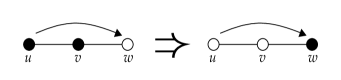
Although this paper only discusses trees, we will describe the basics of pegging for general graphs. Let be a graph, and imagine that several of its vertices are filled with one peg each. Then we consider this set of filled vertices to be a distribution of pegs on . Given distributions and on , we say that is a pegging move from to if there exist distinct vertices and with both and adjacent to and with . Informally, describes the act of the peg on jumping over the peg on and landing on , as shown in Figure 1 below.
In this case we write . If is achieved after performing a finite sequence of pegging moves on , we write . We denote the sequence of the first moves in by for . We say that is reachable (or can be pegged) from a distribution if there exists a finite sequence of pegging moves with . The reach of a distribution on is the set of all vertices reachable from . We say that can be pegged by if . If the graph is clear from the context, we will denote the reach of as simply .
We will now introduce our main definitions.
Definition 2.1.
The pegging number of a graph is the smallest natural number such that is peggable by every distribution of size . The optimal-pegging number of is the minimum size of all distributions on that can peg .
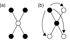
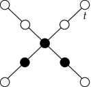
To illustrate these concepts, consider , the star graph on vertices (see Figure 2). Suppose our distribution is . Since no two vertices in are adjacent, it is impossible to perform any pegging moves. Therefore, the center vertex cannot be reached. So there exists a distribution of pegs on such that , which implies that .
Now suppose consists of only two pegs with one placed on the center vertex and one placed on one of the leaves. Since all of the leaves in are adjacent to the center vertex, they can all be reached. So . Since we can’t perform any pegging moves if , .
The next set of definitions is useful for calculating the pegging and the optimal-pegging numbers of a graph.
Definition 2.2.
Let . The weight of a vertex with respect to is , where and is the distance between vertices and . The weight of a distribution with respect to is
The summed weight of a vertex with respect to is
Similarly for , .
Notice that defined in this way is a positive solution of the . Weights satisfy the first of the following two monotonicity lemmas. The second monotonicity lemma establishes that removing pegs from a distribution cannot help us reach vertices that we otherwise could not reach with their presence.
Lemma 2.3 (Monotonicity of Weight).
Let be a distribution of pegs on a graph , and let be the distribution achieved by performing the finite sequence of pegging moves . Then for all .
Lemma 2.4 (Monotonicity of Reach).
Let be two distributions on a graph . Then we have .
See [2] for proofs.
Combining Lemma 2.3 with the fact that if , , we get the following theorem:
Theorem 2.5.
If and , then .
The contrapositive of this theorem is extremely useful for calculating lower bounds for pegging and optimal-pegging numbers. Here is another variation of this theorem.
Corollary 2.6.
If , then .
Proof.
Suppose . Then
∎
Corollary 2.6 shows that we can obtain a lower bound for the optimal-pegging number of any graph by choosing and taking the partial sum of the largest summed weights of the vertices in with respect to . We sum until we achieve some where .
One interesting variation of pegging involves stacking more than one peg on a single vertex. We define a multi-distribution of pegs on a graph as a multiset of the elements of . Informally, is a distribution of pegs on where each vertex can be covered with more than one peg. To distinguish between a multi-distribution and our original definition of a distribution, we will call distributions that only allow one peg per vertex proper distributions. A stacking move from a multi-distribution is a pegging move without the constraint that . Notice that all pegging moves are stacking moves, but the converse is not true. Also notice that the definitions of pegging numbers and optimal-pegging numbers require that the initial distributions of pegs be proper. We say that supersedes if the presence of peg implies that . The set of vertices that are reachable by via stacking moves is denoted .
Let be a multi-distribution of pegs and let be a sequence of stacking moves with . Fix a peg . Informally, we define the ancestors of , denoted , as the set of pegs in that contribute to the placement of . Formally, we define the ancestor function by induction:
-
(1)
If , then .
-
(2)
If , then .
-
(3)
If the specific occurrence of is also in , then
Lemma 2.7.
Let be a distribution of pegs and let be a sequence of moves to obtain some distribution containing pegs . Then .
Proof.
Let be the first moves in where and denote the distribution we achieve after as . Informally, we define the function des as the peg in that is contributed to by some peg in . Formally, we define where we define function by induction:
-
(1)
If peg , then .
-
(2)
If , then .
-
(3)
If , then .
Since preimages of distinct vertices under des are disjoint, the sets and are disjoint. ∎
The following lemma provides a property about pegging graph that we will use frequently in the remainder of this paper.
Lemma 2.8.
Let , and let be a distribution of pegs on . Suppose is a sequence of pegging moves such that . Then for a vertex there exists a path such that .
Proof.
Suppose . If we use to reach then there must exist a path between the two vertices, and the above statement is trivially true. Suppose . In order for a peg to reach , there must be a vertex that is an ancestor of , which implies that there is a path between and . So by transitivity, there is a path from to containing . ∎
The following lemma shows that stacking pegs does not extend the reach of a proper distribution.
Lemma 2.9 (Stacking Lemma).
Let be a proper distribution, and let be a sequence of stacking moves leading to a multi-distribution . Then there exists a sequence of pegging moves resulting from a reordered subsequence of such that the proper distribution supersedes . Moreover, .
See [2] for proof.
Another graph game that is similar to pegging is pebbling. A pebbling move on a multi-distribution is one where we remove two pegs from one vertex and place one on an adjacent vertex. A peggling move is either a stacking move or a pebbling move. The set of vertices that are reachable by via peggling moves is denoted .
The next lemma found in [2] shows that pebbling does not increase the reach of a proper distribution either.
Lemma 2.10 (Peggling Lemma).
Let be a proper distribution and let be a sequence of peggling moves leading to a multi-distribution . Then there exists a sequence of pegging moves such that the proper distribution supersedes . Moreover, .
Since these peg moving methods do not change the reach, they are useful techniques that will come in handy later on.
3. General Trees
In the sections to come, we will introduce various types of trees and compute their pegging numbers and optimal-pegging numbers. The goal of this section is to present two results that are true for all trees. The first result is due to M. Wood [4].
Lemma 3.1.
Let be a tree, and let be a vertex in that is reachable from some distribution . Then is reachable from using only pegging moves toward , i.e. for each move .
The idea behind the proof is that since is acyclic there exists only one path between and . Therefore if we move away from we will eventually have to move toward on the same path, and so such a move would unnecessary.
The second result in this section pertains to the pegging numbers of subtrees.
Lemma 3.2.
Let be a tree and a subtree of . Then .
Proof.
Let . If , then trivially . If , then let be a distribution of size on . By definition of , . Suppose there exist vertices and such that we cannot reach without first reaching . By Lemma 2.8 this can only occur if there exists a path between and some vertex that contains . Since is acyclic, there exists at most one path from to , which is contained in . So is not contained is this path, which implies that . Hence, . ∎
Note that this property of pegging numbers does not hold for general graphs. Nor does the same conclusion hold for optimal-pegging numbers of graphs, trees or otherwise.
4. Complete Binary Trees
In this section we will find bounds for the pegging number and optimal-pegging number of the complete binary tree. We will denote the complete binary tree of height as . A vertex is located at level of if , where is the root of the tree. By this terminology, the root is the vertex located at level 0. We will use the notation to signify that vertex lies at level .
The following lemma is pivotal for calculating a lower bound for the pegging number of these trees.
Lemma 4.1.
If denotes the root of , then
Proof.
A vertex at level is a distance of away from the root. Furthermore, the number of vertices at level is . So
∎
Now we will present our bound.
Theorem 4.2.
Let be a complete binary tree of height . Then for sufficiently large we have
Proof.
By Lemma 4.1, each subtree of of height , denoted , rooted at a vertex has weight . For each leaf there exists a subtree of height whose root is located a distance of away from it. We find this tree by following the path of length from toward the root. Once we are a distance of away from at some vertex , we go to the child of that we have not traversed. This child is at level and therefore is the root of a subtree of height . Since this subtree is a distance from , its weight with respect to is
Let us sum up the weights with respect to of every subtree of height that is a distance of away from . Since is a binary tree, there exists only one such tree of each height that fits these criteria and all of these trees are disjoint. In addition, let us add the weights with respect to of each vertex along the path between and the root which is a distance of from for . In other words, we are adding the weights with respect to of every vertex in and subtracting the subtree of height 7 that contains as a leaf. The weight of this distribution is
As ,
So by Theorem 2.5, we have , which implies that . Since , for sufficiently large we have
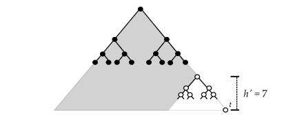
Now let us refine our results. When , we have exactly 1 pegged vertex a distance of 8 from , 2 pegged vertices a distance of 9 from , 4 pegged vertices a distance of 10 from , and 8 pegged vertices a distance of 11 from in the distribution . In there are 64 vertices of distance 12 from , 32 vertices of distance 13 from , and 48 vertices of distance 14 from . If we remove all pegs from vertices of of distances 8, 9, 10, and 11 from and add pegs to all the vertices in of distances 13 and 14 from and 1 of the 48 vertices of distance 12 from , we get a distribution such that
So by Theorem 2.5, , which implies that . Since , for sufficiently large we have
∎
Corollary 4.3.
Corollary 4.4.
Let be a complete binary tree of height . Then
for all .
Proof.
If then this statement is trivially true. Therefore, assume . Then is a subtree of , a complete binary tree that we consider to have a “sufficiently large height.” Let be a distribution of pegs on and a distribution of pegs on . We use the construction of described in Theorem 4.2 so that there exists at least one vertex that we cannot reach. If , then we can construct in such a way that contains the tree of height 7 that was originally unpegged. In accordance of our refined results, at least 157 of the pertinent 172 vertices are unpegged. So , and by Monotonicity of Reach, . Hence, , and . ∎
The next two lemmas are necessary for calculating bounds for the optimal-pegging number for .
Lemma 4.5.
Let be a complete binary tree, and let be the set of leaves of . Then for any vertex where is at level , we have
Proof.
We prove this by strong induction on .
Base Case: . The root is the only vertex in that is located at level 0. Since is complete, all of the leaves in are located at level , and so for all leaves , . Hence,
Inductive Hypothesis: Assume that for all vertices at level that is at most , we have
Inductive Step: Consider the vertex located at level of . The subtree rooted at has a height of , and so by the base case the summed weight of its leaves is . For every other leaf in , the summed weight of is the summed weight of the vertex adjacent to at level multiplied by , since is a distance of 1 away from . However, when we add we have double counted the leaves of the subtree rooted at . We must therefore subtract . So our summed weight for with respect to is:
∎
We proceed using the technique following Corollary 2.6 to find a lower bound for the optimal-pegging number. Our first step is to rank each level of the tree according to the weights of its vertices. In other words, the highest ranking level is the one that contains the vertex with the largest weight, the second highest ranking level is the one that contains the vertex with the second largest weight, and so on. Since every two vertices in the same level have the same weight, a complete ranking exists.
Lemma 4.6.
Let be a complete binary tree, and let be the set of leaves of . If denotes an arbitrary vertex at level in , then for , we have
Proof.
Let and be vertices at levels and of respectively. Then by Lemma 4.5,
So when , i.e. for . Therefore, the summed weight of each vertex decreases as the level of the vertex increases, except when the level increases from 0 to 1.
Now all we need to prove is that . This can be shown directly by calculating the ratios between the weights:
Therefore, . Finally, we calculate the ratio of to :
Thus, . ∎
We are now ready to present our bounds on the optimal-pegging number of .
Theorem 4.7.
For a complete binary tree of height , .
Proof.
Let us first prove the lower bound. Let be the set of leaves of . Since , by Lemma 4.6 we know that the levels of vertices with the largest summed weights with respect to are levels 0 through . Let denote a vertex in level . Since each level has vertices, we can calculate the summed weight with respect to of the distribution made up of all the vertices in the first levels:
So .
The upper bound can be established simply by putting pegs on every vertex of levels 0 through 5 of a tree of height 8. It is possible to reach all the vertices, and since is a subtree of any complete binary tree of height greater than 8, this result can be generalized to all complete binary trees of height at least 8. Furthermore, if we extend a path from the root of a complete binary tree of height 5 with pegs on every vertex of the tree, we can reach a distance of 4 along the path. So given a tree of height 12, if levels 4 through 9 are covered with pegs, we can reach all the vertices in the tree. Therefore, , and so . ∎
5. Infinitary Trees
A complete infinitary tree of height is a tree rooted at a vertex such that each vertex has a countably infinite number of children and the distance between and any leaf is . Since each level consists of an infinite number of pairwise non-adjacent vertices, it is impossible to calculate the pegging number of such a tree in any meaningful way.
However, finding specific finite distributions of pegs that can peg any vertex in the tree is within our reach. In this section we compute the optimal-pegging number of the complete infinitary tree of height .
Lemma 5.1.
Let denote a complete infinitary tree of height rooted at vertex , and let denote the th Fibonacci number. Then any distribution which pegs levels 0 through requires at least pegs. Moreover, .
Proof.
We prove this by strong induction on . Since the base cases are trivial, we assume that the theorem statement is true for all , where . Let be a minimal distribution needed to reach levels 0 through of . Since has finitely many pegs, by the Pigeonhole Principle, there exists at least one subtree of rooted at a child of with no vertices in .
Let be a vertex at level in this subtree of , and let be a minimum finite sequence of pegging moves used to reach from . The last move is for some two vertices in level and in level . By Lemma 2.7, we can partition into two distributions, one that can peg and one that can peg . Suppose . Then neither of the parts contain , and by the inductive hypothesis, they each contain at least and vertices, respectively. This implies that . So in order for to be of size , it must contain .
However, since both partitions cannot contain , one must be sub-optimal. It is evident that if we can place a peg on a vertex in the th level of this subtree, then we are able reach all the vertices in the first levels of the subtree. Then
The distributions for and are obvious. Now we will show how to recursively construct a distribution of size which pegs level 0 through for a tree of height where .
Let be an infinitary tree of height and let where and are optimal distributions for pegging the first level and the first level of , respectively, and are not contained in or , and is adjacent to both and . Since is an infinitary tree, we can choose and so that they intersect only at . We can use to reach any vertex a distance of away from , and to reach any vertex a distance of away from . If we choose to use to peg , the vertex a distance of away from and adjacent to , then we can perform the pegging move where is a vertex adjacent to that is a distance of away from . So we can reach any vertex in levels 0 through of . The size of this distribution is
∎
Theorem 5.2.
Let be an infinitary tree of height . Then
where denotes the th Fibonacci number.
Proof.
By combining our results from Theorems 4.7 and 5.2, we are confronted by the surprising and counterintuitive reality of the existence of trees which have optimal-pegging numbers that increase with the removal of a leaf. We show this in the following corollary.
Corollary 5.3.
There exist infinitely many trees which have optimal-pegging numbers that increase with the removal of a leaf.
Proof.
Let and denote a complete binary tree and an infinitary tree, respectively, both of which have height . By Theorems 4.7 and 5.2, provided that , or
This is true if
or equivalently
This is true for . Since , is a monotonically decreasing function. Hence for all .
Let be the recursively defined distribution on the infinitary tree described in the proof of Lemma 5.1. By Lemma 5.1, the root of is covered with a peg, and the distance between every vertex in and the root is at most 2. Therefore, there exists a complete -ary tree of height , , such that is a subtree of , and . By Lemma 3.1, there exists a finite sequence of pegging moves such that for every . Therefore, for all . Since is finite, by the Pigeonhole Principle, there exists at least one tree that is a subtree of and a supertree of such that the deletion of a leaf from results in a tree with a larger optimal-pegging number. ∎
6. Caterpillars and Lobsters
This section is devoted to computations of the optimal-pegging numbers of caterpillar graphs, as well as calculating the lowest upper bound on the optimal-pegging number of lobster graphs. A caterpillar graph, , is a tree such that if all leaves and their incident edges are removed, the remainder of the graph forms a path. A lobster graph, , is a tree such that if all leaves and their incident edges are removed, the remainder of the graph is a caterpillar.
Theorem 6.1.
The caterpillar graph satisfies , where is the diameter of .
First we need four lemmas that will be used in the proof of this theorem.
Lemma 6.2.
Let be a path on vertices and let be a distribution of pegs on . Then for all , or is adjacent to some vertex in .
Proof.
Suppose that this claim is false, and that there exists a vertex that is a distance of at least two from any vertex in . If , then it must be reachable from the distribution of pegs on one side of it. Let be the distribution of pegs on one side of . We can get an upper bound for the weight of :
Therefore , and so . ∎
Lemma 6.3.
Let be a distribution of pegs on some caterpillar with diameter , and let be a longest path of . If , then .
Proof.
By definition of a caterpillar, a vertex that does not lie in must be a leaf. Let be such a leaf, and let be adjacent to . Assume for the sake of contradiction that . Since is not a leaf there exists two vertices and adjacent to that are in , and are therefore in the reach of . Suppose there exists a sequence of moves where . Then there must be some (possibly ) adjacent to such that either or , for some . Either way, we can reach via the pegging move . The same argument holds if there exists a sequence of moves where . Now suppose this is not the case, and that no such sequence of moves exists where is an ancestor of or . Let us consider the case where there exists a sequence of moves where . If there is some finite sequence of pegging moves such that , since lies in the path between and , and is adjacent to , then for some and . So we can construct a sequence of pegging moves where if and otherwise, and we can reach . If such a sequence does not exist, then by Lemma 2.7, there exists another sequence such that and are disjoint. Let . Then , and so we can reach via the pegging move . If is not an ancestor of and vice versa, we can reach via the pegging move . So . ∎
Lemma 6.4.
Let be a caterpillar with diameter , and let be a distribution of pegs on such that . Denote the set of leaves in as . If , then there exists a distribution such that , , and .
Proof.
Let be a leaf in and be the vertex adjacent to . There are three possible configurations of :
Case 1: . Since is not adjacent to any other pegged vertices, it cannot be used to reach . So . If , then after a series of stacking moves we can achieve 2 pegs on with which to perform a pebbling move to reach . But by the Peggling Lemma, this means that . Furthermore, the set of vertices that can be reached by a pegging move using are all adjacent to , so they can be reached with pebbling moves as well. So .
Case 2: . Suppose there exists a path of length such that . If , then by Lemma 6.3, . Suppose . Since , there is a vertex that is distinct from and adjacent to , and we can perform the stacking move . So , and by Lemma 6.3, .
Suppose no such path exists. Denote the two closest unpegged, non-leaf vertices on opposite sides of as and (in other words, lies on the path between and , and there is no unpegged, non-leaf vertex such that lies on the path between and or and ). Let denote the longest path of containing , , and . By the definitions of and , any other unpegged vertex in is closer to either or than it is to . Suppose is closer to . By Lemma 3.1, if is used to reach , we move the peg on toward , and therefore toward . So if is the sequence of moves on used to reach by first moving the peg on , and if is the smallest index such that contains , then . Since the pegs on and are removed from in the first moves of , . Let . Then , and so . We can follow a similar argument if is closer to . So , and by Lemma 6.3, . ∎
The following lemma and its proof were presented in Helleloid, et al. [2].
Lemma 6.5.
For , the path satisfies .
Proof of Theorem 6.1.
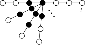
The optimal-pegging numbers for lobsters are not as straightforward. A caterpillar is a type of lobster, so some lobsters with diameters have optimal-pegging numbers as low as . However, this is not the case for all lobsters. A counterexample is a lobster such that if all its leaves and their incident edges are removed, the remainder of the graph is a star with at least 4 leaves. The diameter of this graph is 4, and so for the sake of contradiction, suppose we only need a distribution , of 3 pegs to reach all the vertices in . By the Pigeonhole Principle, there is at least one leaf such that where is the closest vertex to in , and no other vertex in is as close to as is. The closest we can get a peg to after one move is a distance 1 away from . However, since the third peg is a distance of at least 3 away from , the two pegs remaining on the graph are not adjacent, and so no more pegging moves can be performed. Therefore, 3 pegs are not sufficient to peg .
For this reason, we present only an upper bound for the optimal-pegging number of a lobster.
Theorem 6.6.
For all lobsters with diameter , we have .
Proof.
Consider the distribution where all the pegs cover a longest path of with the exception of the two endpoints. Clearly, if we can reach every leaf in , then we can reach all the vertices in . Since , any vertex in, or adjacent to, some vertex in is reachable, so let us consider the case where the leaf in question is a distance of at least two away from any vertex in . Let where is the leaf, , and is adjacent to both and . Since we know that there are two vertices and adjacent to that are covered with pegs. Furthermore, since , there must exist another vertex adjacent to either or in . Without loss of generality, assume that is adjacent to . Then we can reach via a series of pegging moves:
So . ∎
7. Future Research and Acknowledgments
Future research includes finding bounds on complete -ary trees for . We can also study various types of caterpillars and lobsters in greater depth. By classifying these graphs by properties such as the number of their leaves, their diameters, or the regularity of their constructions, one might be better able to compute their pegging numbers. Another direction would be to find the probabilities that specific graphs can be pegged based on the size of their distributions with respect their number of the vertices.
The research for this paper was conducted at the University of Minnesota Duluth and was made possible by the financial support of the National Security Agency (grant number DMS-0447070-001) and the National Science Foundation (grant number DMS-0447070-001). I would like to extend special thanks to Ricky Liu, Reid Barton, and David Moulton for the ideas, suggestions, and intellectual support that they provided, and to Joe Gallian for proposing the topic of this paper and for running the REU at the University of Minnesota Duluth. I would also like to thank David Arthur, Mike Develin, Stephen Hartke, Geir Helleloid, Philip Matchett-Wood, Joy Morris, Julie Savitt and Melanie Wood for their input and suggestions.
References
- [1] E. R. Berlekamp, J. H. Conway, R. K. Guy, Winning Ways for Your Mathematical Plays, Academic Press, London, 1982, vol. 2, .
- [2] G. Helleloid, M. Khalid, P. Matchett, and D. Moulton, Graph pegging numbers, to appear in Discrete Mathematics, 2005.
- [3] G. H. Hurlbert, A survey of graph pebbling, Congr. Numer. 139 (1999), .
- [4] M. Wood, Graph pegging and graph powers, personal communication.