MaNN: Multiple Artificial Neural Networks
for modelling the Interstellar Medium

Abstract

Aims. Modelling the complex physics of the Interstellar Medium (ISM) in the context of large-scale numerical simulations is a challenging task. A number of methods have been proposed to embed a description of the ISM into different codes. We propose a new way to achieve this task: Artificial Neural Networks (ANNs).

Methods. The ANN has been trained on a pre-compiled model database, and its predictions have been compared to the expected theoretical ones, finding good agreement both in static and in dynamical tests run using the Padova Tree-SPH code EvoL.

Results. A neural network can reproduce the details of the interstellar gas evolution, requiring limited computational resources. We suggest that such an algorithm can replace a real-time calculation of mass elements chemical evolution in hydrodynamical codes.

1 Introduction

In the framework of modern large-scale numerical hydrodynamical simulations, the correct modelling of the Interstellar Medium (ISM) plays an increasingly crucial role as many physical phenomena such as star formation, energy feedback, diffusion of heavy elements and others, strongly depend on it and simultaneously affect the properties of the ISM. The task is, however, very demanding. This is ultimately due to the complexity of the hydrodynamical interactions of the Baryonic Matter in large scale systems. Contrary to the simple behaviour of the Dark Matter dynamically governed only by gravity, the behavior of the Baryonic Matter is the result of many complex and interwoven physical phenomena. Therefore, to obtain a realistic model of the ISM, many physical processes must be taken into account going from chemical reactions among atoms and molecules occurring in complicated networks, dust formation and destruction, chemical reactions taking place on dust grains, to heating and cooling by various mechanisms, photo-ionization and radiative transfer. These processes span wide ranges of temperature and density, thus making their accurate, simultaneous description a cumbersome affair.

Moreover, even when the physics is described with the desired accuracy, the number of mass elements (particles) customarily used in large-scale simulations is large (typically $10^{4}$ to $10^{7}$), so that large amounts of computational workload are requested. Clearly, computing the internal evolution of each mass element in detail is extremely time-consuming, whatever the method chosen to follow it might be.

The aim of this study is to present a method able to alleviate part of the above difficulties by approximating the exact solution of a detailed physical model and yet ensuring both a robust and sufficiently precise description of the gas properties, while maintaining the computational workload to an acceptable level.

The method stands on the model of the ISM and companion code Robo developed by Grassi et al. (2010). In brief, Robo follows the evolution of a gas element during a given time interval $\Delta t$. In other words, given the initial physical and chemical state of a gas element as functions of its hydrodynamical properties, the relative abundances of its chemical constituents and the kind of interactions with the surrounding medium, the model calculates the final state after some time interval $\Delta t$.

The straight implementation of Robo into a generic hydrodynamical simulation (and companion code) to perform the on-the-fly computation of the ISM properties, although desirable, would be far too expensive in terms of computational costs. The easiest way of proceeding would be to store the results of Robo as look-up tables (grids) where the values of interest (e.g. the physical parameters of the gas element: mass fractions of molecular, neutral, ionized hydrogen; temperature, density, pressure; the abundance of dust, and so on) are memorized for a given (large) set of initial configurations. However, each parameter to be stored corresponds to one dimension of the look-up table (grids). Thus, tracking $N$ parameters requires a $N$-dimensional matrix. Such matrix is discrete, so an interpolation in a $N$-dimensional space is required to know the final state corresponding to a given initial state of a generic gas element. The all procedure when applied many times to a high number of gas particle would be very time consuming. A different strategy must be conceived.

To cope with this, we develop an algorithm based on the Artificial Neural Networks (ANN) technique to establish the correspondence between the initial $+$ final state. The ANN technique can handle a large number of parameters without requiring a real-time interpolation. The ANNs require few floating point operations and “learn” to behave like the original physical models on which they are trained. The computational cost of it is easily affordable.

The paper is organized as follows. In Section 2 we briefly describe the ISM model and companion code Robo. In Section 3 we briefly review the concept and algorithm of the ANN in general, whereas in Section 4 we present the ANN we have set up for our purposes. This is named MaNN. In the same section, we also examine the ability of MaNN in reproducing the data calculated by Robo. In Section 5 we describe how MaNN is implemented into the NB-TSPH code EvoL of Merlin et al. (2010) and present a suitable hydrodynamical test aimed at checking the robustness of the method. Finally, in Section 7 we summarize our results and draw some general considerations.

2 Robo: the ISM model and companion code

Robo is a numerical code specifically designed to study the evolution of the ISM. It includes several atomic and molecular species linked together by a large network of reactions. In the following we summarize the main features of Robo and emphasize the fact that Robo is specifically tailored to follow the evolution of the coolants owing to their important role in the wider context of the ISM evolution. To this purpose, we follow the temporal variation of molecules like $\mathrm{H}_{2}$, $\mathrm{HD}$ and metals like C, O, Si, Fe and their ions. For all the details the reader should refer to Grassi et al. (2010).

Layout of the ISM model. The model deals with an ideal ISM element of unit volume, containing gas and dust in arbitrary initial proportions, whose initial physical conditions are specified by a set of parameters, which is let evolve for a given time interval. The history leading the element to that particular initial physical state is not of interest here. The ISM element is mechanically isolated from the host environment, i.e. it does not expand or contract under the action of large scale forces, however it can be interested by the passage of shock waves originated by physical phenomena taking place elsewhere (e.g. supernova explosions). Furthermore, it does not acquire nor lose material, so that the conservation of the total mass applies, even if its chemical composition can change with time. It is immersed in a bath of UV radiation generated either by nearby or internal stellar sources and in a field of cosmic ray radiation. It can generate its own radiation field by internal processes and so it has its own temperature, density and pressure, each other related by an Equation of State (EoS). If observed from outside, it would radiate with a certain spectral energy distribution. For the aims of this study, we do not need to know the whole spectral energy distribution of the radiation field pervading the element, but only the UV component of it. Given these hypotheses and the initial conditions, the ISM element evolves toward another physical state under the action of the internal network of chemical reactions changing the relative abundances of the elemental species and molecules, the internal heating and cooling processes, the UV radiation field, the field of cosmic rays, and the passage of shock waves. The model is like an operator determining in the space of the physical parameters conditions the vector field of the local transformations of the ISM from one initial state to a final one. This is the greatest merit of this approach, which secures the wide applicability of the model.

The chemical network. The following species are tracked by Robo: $\mathrm{H}$, $\mathrm{H}^{+}$, $\mathrm{H}^{-}$, $\mathrm{H}_{2}$, $\mathrm{D}$, $\mathrm{D}^{+}$, $\mathrm{D}^{-}$, $\mathrm{D_{2}}$, $\mathrm{HD}$, $\mathrm{HD}^{+}$, $\mathrm{He}$, $\mathrm{He}^{+}$, $\mathrm{He}^{++}$, $\mathrm{C}$, $\mathrm{C}^{+}$, $\mathrm{O}$, $\mathrm{O}^{+}$, $\mathrm{Si}$, $\mathrm{Si}^{+}$, $\mathrm{Fe}$, $\mathrm{Fe}^{+}$, and $\mathrm{e}^{-}$. The list of reactions and their rates that are included in Robo can be found in Grassi et al. (2010). The reactions are of different type and can be grouped as follows

• collisional ionization ($\mathrm{A}+\mathrm{e}^{-}\to\mathrm{A}^{+}+2\mathrm{e}^{-}$),

• photo-recombination ($\mathrm{A}^{+}+\mathrm{e}^{-}\to\mathrm{A}+\gamma$),

• dissociative recombination ($\mathrm{A}^{+}_{2}+\mathrm{e}^{-}\to 2\mathrm{A}$),

• charge transfer ($\mathrm{A}^{+}+\mathrm{B}\to\mathrm{A}+\mathrm{B}^{+}$),

• radiative attachment ($\mathrm{A}+\mathrm{e}^{-}\to\mathrm{A}^{-}+\gamma$),

• dissociative attachment ($\mathrm{A}+\mathrm{B}^{-}\to\mathrm{AB}+\mathrm{e}^{-}$),

• collisional detachment ($\mathrm{A}^{-}+\mathrm{e}^{-}\to\mathrm{A}+2\mathrm{e}^{-}$),

• mutual neutralization ($\mathrm{A}^{+}+\mathrm{B}^{-}\to\mathrm{A}+\mathrm{B}$),

• isotopic exchange ($\mathrm{A}^{+}_{2}+\mathrm{B}\to\mathrm{AB}^{+}+\mathrm{A}$)

• dissociations by cosmic rays ($\mathrm{AB}+\mathrm{CR}\to\mathrm{A}+\mathrm{B}$),

• neutral-neutral ($\mathrm{AB}+\mathrm{AB}\to\mathrm{A}_{2}+\mathrm{B}_{2}$),

• ion-neutral ($\mathrm{AB}^{+}+\mathrm{AB}\to\mathrm{AB}_{2}^{+}+\mathrm{A}$),

• collider ($\mathrm{AB}+\mathrm{C}\to\mathrm{A}+\mathrm{B}+\mathrm{C}$),

• ionizations by field photons ($\mathrm{A}+\gamma\to\mathrm{A^{+}}+\mathrm{e^{-}}$)

where $\mathrm{A}$ and $\mathrm{B}$ are two generic atoms, $\gamma$ is a photon. Note that cosmic rays and photo-ionization effects are included.

Dust. Robo also tracks the evolution of dust, in turn made by several components, of which it follows the formation and destruction. The formation of dust is modelled according to the prescriptions by Dwek (1998), however with some modifications that allow us to know when a species belonging to the gas phase is captured by dust (trapped at the surface of dust grain lattice). The evolution of the dust type (both in abundance and dimensions) is followed for silicates and carbonaceous grains. Dust is also destroyed by thermal sputtering and shocks. The first process is modeled using the description by Draine & Salpeter (1979), that depends on the environment density and the grain size. We also add the dependence on temperature, considering that hot gas disrupts the dust grains more efficiently than the cold one. The dust disruption by shocks requires the velocity distribution of the gas component to be known. This is supposed to be in the turbulence regime and the velocity field to be suitably described by the Kolmogorov-law. This allows us to describe the shocks on very small scales (contrary to what usually happens in large-scale simulations that do not have the required spatial resolution). Dust is an important component of the ISM because it affects the formation of $\mathrm{H_{2}}$ (one of the most efficient coolants of the ISM) and $\mathrm{HD}$ and also the gas phase catalyzing some chemical processes. The formation of $\mathrm{H_{2}}$ and $\mathrm{HD}$ is modeled as in Cazaux & Spaans (2009), whose description depends on the gas and dust temperature. Finally, the photoelectric ejection of electrons from dust grains is described in detail as well. We can estimate the amount of heating (and cooling) produced by each size-bin of the grain distribution. For further details, see Grassi et al. (2010).

Cooling. Several cooling processes are considered in Robo. In the high temperatures regime ($T\geq 10^{4}$ K) the metallicity dependent cooling rates of Sutherland & Dopita (1993) are adopted. For temperatures lower than $10^{4}\,\mathrm{K}$ we consider the following processes: (i) cooling by molecular hydrogen according to the formulation by Galli & Palla (1998), however, supplemented by the results of Glover & Jappsen (2007) who take in account the $\mathrm{H_{2}}-\mathrm{H}$ interaction and the collisions with $\mathrm{He}$, $\mathrm{H^{+}}$, $\mathrm{H_{2}}$ and free electrons; (ii) cooling by metals is modeled including C, Si, O, Fe, and their ions as in Maio et al. (2007), Glover & Jappsen (2007) and Hollenbach & McKee (1989); (iii) cooling by deuterated molecular hydrogen according to the model by Lipovka et al. (2005); (iv) cooling by the CO molecule and (v) finally, cooling by Cen (1992).

The total cooling rate is the sum of all the contributions

$$\Lambda_{\mathrm{tot}}=\Lambda_{\mathrm{SD}}+\Lambda_{\mathrm{H}_{2}}+\Lambda_{\mathrm{HD}}+\Lambda_{\mathrm{CO}}+\Lambda_{\mathrm{metals}}+\Lambda_{\mathrm{CEN}}\,,$$

where the various terms $\Lambda s$ are all functions of temperature and density and $\Lambda_{\mathrm{SD}}$ is the cooling rate by Sutherland & Dopita (1993), $\Lambda_{\mathrm{H}_{2}}$, $\Lambda_{\mathrm{HD}}$ and $\Lambda_{\mathrm{CO}}$ are the cooling rates of the indicated molecular species, and $\Lambda_{\mathrm{metals}}$ is the cooling by metals (C, O, Si and Fe). Finally, $\Lambda_{\mathrm{CEN}}$ is the cooling by Cen (1992).

It is worth to notice that in the tests presented in this paper the cooling proposed by Cen (1992) is disabled (i.e. $\Lambda_{\mathrm{CEN}}=0$).

Heating. For the photo-dissociation of the molecular hydrogen and the UV pumping, the H and He photo-ionization, the $\mathrm{H_{2}}$ formation in the gas and dust phase and, finally, the ionization from cosmic rays, heating is described as in Glover & Jappsen (2007). For the heating due to the photoelectric effect on dust grains, the model proposed by Bakes & Tielens (1994) and Weingartner & Draine (2001) is used.

Integration time of the models. Each model of the ISM is followed during a total time of about $10^{4}\ \mathrm{yr}$. This choice stems from the following considerations. Each model of the ISM is meant to represent the thermal-chemical history of a unit volume of ISM, whose initial conditions have been established at certain arbitrary time and whose thermal-chemical evolution is followed over a time scale comparable to the maximum time step of the TreeSPH code. The initial physical conditions are fixed by a given set of parameters each of which can vary over wide ranges. One has to solve the network of equations for a time scale long enough to reveal the variations due to important phenomena such star formation, cooling and heating, but not long to allow to the system to depart from the instantaneous situation one is looking at. The value of $10^{4}$ yr resulted to be a good compromise. The initial value of the time-step is $1\ \mathrm{yr}$. This time-step determines the minimum number of steps required to cover the time spanned by a model. It means that each simulation needs at least $10^{4}$ iterations to be completed. The numerical integrator may introduce shorter time steps depending on the complexity of the problem. This value for the time-step seems to keep the system stable during the numerical integration.

Database of models. Varying the initial value of the parameters describing the ISM (such as the temperature, density, abundances of elemental species etc.), Robo is used to create a large number of evolutionary models.

3 The Artificial Neural Networks

As already mentioned, the ideal way of proceeding would be to insert Robo into a code simulating the temporal evolution of large scale structures and to calculate the thermodynamical properties of the ISM component. In all practical cases, this would be unreasonably time consuming. To cope with it without loosing accuracy in the physical description of the ISM we construct an ANN able to replace Robo in all cases.

In brief, ANNs are non-linear tools for statistical data modeling, used to find complex relationships between input and output data or to discover patterns in complex datasets. The first idea of an ANN is by Hebb (1949). In the early sixties Rosenblatt (1962) built the first algorithm based on the iterative penalty and reward method, and finally, after two decades of silence, new ideas were brought by Carpenter & Grossberg (1987, 1987, 1990) (adaptive resonance theory), Hopfield (1982, 1984) (associative neural network) and Rumelhart et al. (1986); McClelland et al. (1986), who developed the back-propagation algorithm, today a common and widely used training scheme.

Demanding computational problems (e.g. multidimensional fits or classifications) can be easily solved using ANNs whereas other methods would require large computing resources. An ANN is based on a simple conceptual architecture inspired by the biological nervous systems. It looks like a network composed by neurons and linked together by synapses (numerical weights). This structure is modeled with a simple algorithm, designed to predict an output state starting from an original input state. To achieve this, the ANN must be trained, so that it can “learn” to predict the output state from a given set of initial configurations. The simplest way of doing it, is the supervised learning: input-output values are fed to the network, then the ANN tentatively computes an output set for each input set, and the difference between the predicted and the original output (i.e. the error) is used to calculate penalties and rewards to the synaptic weights. If the convergence to a solution exists, after a number of iterations, the predicted output value gets very close to the original one: the ANN has learned.

The network stores the original data in some dedicated neurons, the so called input neurons, elaborates these data and sends the results to another group of neurons that are called output neurons. Thus, data flow from input to output neurons. There is another group of neurons, named hidden neurons, that help the ANN to elaborate the final output (see Fig. 1). Each neuron (or unit) performs a simple task: it becomes active if its input signal is higher than a defined threshold. If one of these units becomes active, it emits a signal to the other neurons; for this reason, each unit can be considered as a filter that increases or decreases the intensity of the received signal. The connections between neurons simulate the biological synapses and this is the reason why they are called synaptic weights or, more simply, weights.

The whole process can be written as follows:

$$n_{i}=f(x)\left(\sum_{j}w_{ij}n_{j}-\theta_{i}\right)\,,$$ (1)

where $n_{i}$ is the $i$-th neuron value, $f(x)$ is the activation function, $w_{ij}$ is the weight between $i$-th and $j$-th neuron, $\theta_{i}$ is the neuron threshold, and $x$ is the signal. For the activation function we adopt a sigmoid

$$f(x)=\frac{1}{1+e^{-\beta x}}\,,$$ (2)

where $\beta$ is a parameter fixing the sigmoid slope. It is worth recalling that other expressions for the activation function can be used.

In general the ability of the network to reproduce the data increases with the number of the hidden units up to a certain limit otherwise the ANN gets too “stiff” so that predicting the original output values gets more difficult. The ANN stops learning. Another reason to avoid many hidden neurons is that the procedure becomes time consuming (one must remember that we are mainly dealing with with matrix products). On the other side, an ANN with too few hidden units gets “dull” in reproducing the original data. Therefore, there is an optimal number of hidden neurons for each ANN.

There are several possible ANN architectures, depending on the task the network is designed to perform. The already cited back-propagation algorithm (Rumelhart et al. 1986) is among the most versatile methods, it is one of the most suited to the supervised learning stage and can be applied to a wide range of problems. The name stems from the fact that the error produced by the network is propagated back to its connections to change the synapsis weights and consequently to reduce the error. As a detailed description of the ANN technique is beyond the aims of this paper, we limit ourselves to describe in some detail only the particular algorithm we have adopted for our purposes.

4 MaNN: aims and architecture

MaNN is the network we built to reproduce the ISM output models calculated by Robo. We use a layer of input neurons where each input value corresponds to a free parameter of the Robo models, i.e. the ones shortly described in Sect. 2. The definition of the model in MaNN requires some clarifications. While Robo calculates the whole temporal evolution of a model, MaNN needs only the set of initial parameters (the input model) and the set of final results (the output model). Therefore, a MaNN model is made of two strings (vectors) of quantities: the initial conditions for the key parameters (the input vector) and the results for the quantities describing the final state, after that the assigned time interval has elapsed (the output vector). We refer to the input vector as the vector $\bar{x}$ whose dimension, i.e. the number of input units, is $n_{x}$. We then choose the shape of the output layer of neurons having in mind an “optimal” number of parameters to be used in a typical dynamical simulation. We use $\bar{y}$ to indicate these units and the number of the neurons belonging to this layer is $n_{y}$ . For example, if the code generating the input data only tracks the abundance of neutral hydrogen and the temperature, the MaNN input vector will be $\bar{x}=\left\{n_{\mathrm{H}}^{t},T^{t}\right\}$ and the relative output vector will be $\bar{y}=\left\{n_{\mathrm{H}}^{t+\Delta t},T^{t+\Delta t}\right\}$, and consequently $n_{x}=n_{y}=2$. In this example the number of inputs is equal to the number of outputs, but this is not a strict requirement. In general, to avoid degeneracies one should have $n_{x}\geq n_{y}$ (considering indipendent database parameters). The input parameters can be also different from the output parameters, so in the previous example it could be $\bar{y}=\left\{n_{\mathrm{H}}^{t+\Delta t},n_{\mathrm{H_{2}}}^{t+\Delta t}\right\}$.

There are two more layers in the MaNN, both are hidden and generally with the same size, which in turn depends on the complexity of the task (for example, retrieving a single output value can be obtained with two hidden layers of five elements, or even less). The first layer is $\bar{h}$ with $n_{h}$ neurons and $\bar{g}$ is the second one with $n_{g}$ units. Each layer is connected with a matrix of weights. A $n_{x}\times n_{h}$ matrix named $W_{xh}$ is situated between the input units and the first hidden layer. Similarly, there is a $n_{h}\times n_{g}$ matrix named $W_{hg}$ and, finally, $W_{gy}$, which is a $n_{g}\times n_{y}$ matrix. The architecture of MaNN that we have described here is sketched in Fig. 1.

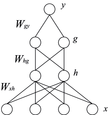
Figure 1: The architecture of MaNN. Circles indicate neurons, lines are connections (i.e. weights). Input units are labeled with the symbol $\bar{x}$, hidden neurons with $\bar{h}$ if they belong to the first layer, and $\bar{g}$ if they belong to the second one; finally, output units are indicated with $\bar{y}$. The matrix $W_{xh}$ represents the weights between input and the first hidden units, $W_{hg}$ are the connections between the first hidden units and the second hidden layer and $W_{gy}$ connects the second layer of hidden units and the output. A single output is shown. In this figure the forward propagation is from lower neurons to the upper ones. Back-propagation is from $\bar{y}$ to $\bar{x}$ neurons. Here $n_{x}=4$, $n_{h}=n_{g}=2$ and $n_{y}=1$.

4.1 The learning stage

The whole learning process is divided into two different steps; the first one is the so called training stage, where MaNN is trained with a randomly chosen set of data. In the subsequent test stage new, blank (i.e. never used before) data are presented to MaNN to verify its behavior and the quality of the training. If MaNN retrieves the new data with a small (user defined) error, than the training stage is terminated. In case the error is still large, a new training stage is required. The training stage can also be stopped if the absolute error starts to increase again after an initial decrease (early-stopping). The aim is to avoid the so called over-training: a network is over-trained when it adapts too strictly to the data fed during the supervised learning, so that it cannot generalize the prediction to reproduce new cases of the test set of data, which contains data patterns that were not present in the previous stage.

At the beginning of the training process, each weight is initialized to a small, randomly chosen, value in the range $[-0.1,0.1]$. The weights change under the action of MaNN. The rate at which MaNN changes its weights, otherwise known as the learning rate $\eta$, must be chosen carefully: for too high a value MaNN could oscillate without reaching a stable configuration, whereas for too small a value MaNN could take a long time to reach the desired solution or, even worse, be trapped in a false minimum of the error hyper-surface. We usually choose $0.1\leq\eta\leq 0.9\,$.

The matrix of initial parameters contains $N$ rows (the initial configurations of the input models); we randomly pick from this set $N_{L}<N$ rows for the training stage, which we refer to as $L$, and $N_{T}=N-N_{L}$ rows for the test stage, $T$.

A set $\bar{s}$ of initial parameters randomly picked up from $N_{L}$ is fed to the network as input vector $\bar{x}=\bar{s}$. The activation of each node belonging to the first hidden layer is then computed as

$$\bar{h}=f\left(\bar{x}\otimes W_{xh}\right)\,,$$ (3)

where $\bar{h}$ is the vector of hidden neurons, $f$ is the sigmoid function, $W_{xh}$ is the weight matrix between the input and the first hidden neurons, and $\otimes$ indicates the matrix product. If $\bar{c}=\bar{a}\otimes B$, where $\bar{a}$ is a vector of $n$ elements and $B$ is a matrix $n\times m$, the size of the vector $\bar{c}$ is $m$. The sigmoid function $f\left(\bar{v}\right)$ has $\beta=1$. Then the following relation holds

$$\bar{g}=f\left(\bar{h}\otimes W_{hg}\right)\,,$$ (4)

with obvious meaning of the symbols. Finally, the output vector of MaNN is given by

$$\bar{y}=f\left(\bar{g}\otimes W_{gy}\right)\,.$$ (5)

This first step is named the forward-propagation, because the algorithm calculates the output of the network for a given input vector $\bar{x}=\bar{s}$.

During the very first forward-propagation the output vector will contain nearly random values, because the weights are randomly generated. To improve upon it, we compute the error and back-propagate it to change the weights accordingly. The error at the output layer is

$$\bar{\delta}_{y}=\left(\bar{t}-\bar{y}\right)\dot{f}\left(\bar{A}_{y}\right)=\left(\bar{t}-\bar{y}\right)\bar{y}(1-\bar{y})\,,$$ (6)

where $\bar{A}_{y}$ is the vector of the activation functions for the output layer and the last equality is valid only with the activation function $f\left(\bar{v}\right)$ with $\beta=1$ that we have adopted. The error $\bar{\delta}_{y}$ is propagated back to the second hidden layer to become

$$\bar{\delta}_{g}=\dot{f}\left(\bar{A}_{g}\right)\left[\bar{\delta}_{y}\otimes W_{gy}\right]=\bar{g}\left(1-\bar{g}\right)\left[\bar{\delta}_{y}\otimes W_{gy}\right]\,,$$ (7)

with obvious meaning of all the symbols and expressions. Finally the error is propagated back for the last time giving

$$\bar{\delta}_{h}=\dot{f}\left(\bar{A}_{h}\right)\left[\bar{\delta}_{g}\otimes W_{hg}\right]=\bar{h}\left(1-\bar{h}\right)\left[\bar{\delta}_{g}\otimes W_{hg}\right]\,.$$ (8)

Now that the error for each step between the various layers has been computed, the changes of the synaptic weights are

$$\Delta W_{xh} = \eta\left[\bar{x}\otimes\bar{\delta}_{h}\right]+\alpha\Delta W_{xh}^{o}\,,$$

$$\Delta W_{hg} = \eta\left[\bar{h}\otimes\bar{\delta}_{g}\right]+\alpha\Delta W_{hg}^{o}\,,$$

$$\Delta W_{gy} = \eta\left[\bar{g}\otimes\bar{\delta}_{y}\right]+\alpha\Delta W_{gy}^{o}\,,$$

The last terms at the r.h.s. of the above equations is called the momentum made by the product of a parameter $\alpha$ (to be tuned) and the variation of the corresponding weights at the previous step. $\Delta W_{xh}^{o}$ and the other similar terms indicate the values of the weights at the previous training step. The momentum is introduced to force the procedure to avoid false minima in the error hyper-surface. This loop must be repeated for each combination of the parameters in the set $L$.

To test the efficiency of the MaNN learning, the forward propagation is then applied to all the variables belonging to the set $L$. The RMS of the test data set is

$$\mathrm{RMS}=\sqrt{\frac{\sum_{i=1}^{N_{T}}\left(y_{i}-t_{i}\right)^{2}}{N_{T}-1}}\,,$$ (10)

where $y_{i}$ is the output for the $i$-th test, $t_{i}$ is the $i$-th correct test pattern and consequentially $y_{i}-t_{i}$ is the MaNN’s error.

The training test loop will be repeated until the MaNN’s learning reaches one of the following cases: (i) the RMS is lower than a certain limit chosen by the user, (ii) the RMS does not change for a sufficient number of loop cycles or, finally, (iii) the early-stopping condition is verified.

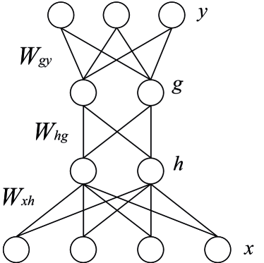
Figure 2: The architecture of a double hidden layer ANN. Circles indicate neurons, while lines represent the connections between the layers (i.e. weights). The input units are labeled with the symbol $\bar{x}$, the hidden neurons with $\bar{h}$ if they belong to the first layer, and with $\bar{g}$ if they belong to the second one; finally, the output units are indicated with $\bar{y}$. The matrix $W_{xh}$ represents the weights between the output and the first hidden units, $W_{hg}$ are the connections between the first hidden units and the second one and $W_{gy}$ connects the second layer of hidden units and the output. Multiple outputs are shown. In this figure the forward propagation is from the lower neurons to the upper ones. The back-propagation is from $\bar{y}$ to $\bar{x}$ neurons. Here $n_{x}=4$, $n_{h}=n_{g}=2$ and $n_{y}=3$.

5 Training and testing MaNN

5.1 Input data from Robo

As already stated, with Robo we have calculated approximately 55000 models. For a given set of initial conditions and physical parameters, each model describes the state of an ISM element after $\Delta t=10^{4}$ years of evolution. This time interval is short enough to secure that only small changes in gas abundances have occurred (a sort of picture of the physical state at given time), and long enough to be compatible with the typical time step in large-scale dynamical simulations.

For the purposes of the present analysis, we limit ourselves to track the following parameters: temperature $T$, metallicity $\tilde{Z}=10^{[\mathrm{Fe}/\mathrm{H}]}$  , and number densities of $\mathrm{H}$, $\mathrm{H}_{2}$, $\mathrm{H}^{+}$ and $\mathrm{e}^{-}$. This means that in addition to the temperature, MaNN is designed here to follow just these four species, whereas Robo can actually follow twenty-three species including atoms, molecules and free electrons. The main motivation for this limitation is that in a large numerical dynamical simulation it is more convenient in terms of computing time and workload to follow in detail only those species (and their abundances) that are known to play a key role in the real evolution of the ISM (with particular attention to star formation and energy feedback) and to consider all the other species to remain nearly constant and small. In brief, the heavy elements are important coolants and the same holds for the molecular hydrogen, at least below $\sim 10^{4}$ K. The ionization fraction of hydrogen is also important, because free electrons are involved in a number of chemical reactions, and are the colliders that excite the coolants: this is the reason why $n_{\mathrm{H^{+}}}$ and $n_{\mathrm{e^{-}}}$ are considered. Moreover, the neutral $n_{\mathrm{H}}$ is in the list to ensure the mass conservation while changing the fractional abundances. Finally, the temperature determines the kind of physical processes that are important.

The initial values of the number densities. The initial values of the number densities fall in three groups: (i) the elemental species with constant initial values, the same for all the models (namely $\mathrm{H^{-}}$, $\mathrm{H_{2}^{+}}$, $\mathrm{He^{+}}$ and $\mathrm{He^{++}}$); (ii) the elemental species whose initial values are derived from other parameters (namely He, all the deuteroids and the metals, like for instance $\mathrm{C}$ and $\mathrm{O}$, that depend on the choice of the total metallicity $\tilde{Z}$) and, finally, (iii) the elemental species with free initial conditions (namely $\mathrm{H}$, $\mathrm{H_{2}}$, $\mathrm{H^{+}}$, and $e^{-}$).

Hydrogen group: $\mathrm{H}$, $\mathrm{H^{+}}$, $\mathrm{H^{-}}$, $\mathrm{H_{2}}$ and $\mathrm{H_{2}^{+}}$. The initial values of the species $\mathrm{H^{-}}$ and $\mathrm{H_{2}^{+}}$ are $n_{\mathrm{H}^{-}}=n_{\mathrm{H}_{2}^{+}}=10^{-10}$cm^-3 Prieto et al. (2008), while the other three hydrogen species have free initial values.

Deuterium group: $\mathrm{D}$, $\mathrm{D^{+}}$, $\mathrm{D^{-}}$, $\mathrm{D_{2}}$, $\mathrm{HD}$ and $\mathrm{HD^{+}}$. The numerical densities of the deuteroids are calculated from their hydrogenoid counterparts. For the single atom species we have $n_{\mathrm{D}}=f_{\mathrm{D}}\,n_{\mathrm{H}}$, $n_{\mathrm{D^{+}}}=f_{\mathrm{D}}\,n_{\mathrm{H^{+}}}$ and $n_{\mathrm{D^{-}}}=f_{\mathrm{D}}\,n_{\mathrm{H^{-}}}$, where $f_{\mathrm{D}}=n_{\mathrm{D}}/n_{\mathrm{H}}$. For the molecules, we can consider the ratio $f_{\mathrm{D}}$ as the probability of finding an atom of deuterium in a population of hydrogen-deuterium atoms. This assumption allows us to calculate the $\mathrm{HD}$, $\mathrm{D}_{2}$ and $\mathrm{HD^{+}}$ number densities as a joint probability; for $\mathrm{HD}$ and $\mathrm{HD}^{+}$ we have $n_{\mathrm{HD}}=f_{\mathrm{D}}\,n_{\mathrm{H_{2}}}$ and $n_{\mathrm{HD^{+}}}=f_{\mathrm{D}}\,n_{\mathrm{H_{2}^{+}}}$, but for $\mathrm{D}_{2}$ is $n_{\mathrm{D_{2}}}=f_{\mathrm{D}}^{2}\,n_{\mathrm{H_{2}}}$ as the probability of finding two deuterium atoms is $f_{\mathrm{D}}^{2}$. This is valid as long as $f_{\mathrm{D}}\ll 1$.

Helium group: $\mathrm{He}$, $\mathrm{He}^{+}$, $\mathrm{He}^{++}$. The ratio $\mathrm{n_{He}/n_{H}}$ is set to 0.08, thus allowing to the initial value of $\mathrm{n_{He}}$ to vary accordingly to the initial value for $\mathrm{n_{H}}$. The initial number densities of the species $\mathrm{He}^{+}$, $\mathrm{He^{++}}$ are both set equal zero and kept constant in all the models.

Metals group: $\mathrm{C}$, $\mathrm{C}^{+}$, O, $\mathrm{O}^{+}$, $\mathrm{Si}$, $\mathrm{Si}^{+}$ and $\mathrm{Fe}$, $\mathrm{Fe}^{+}$. The $\mathrm{Fe}$ number density of the ISM is

$$n_{\mathrm{Fe}}=n_{\mathrm{H}}\cdot\mathrm{dex}\left\{[\mathrm{Fe/H}]+\log\left(\frac{n_{\mathrm{Fe}}}{n_{\mathrm{H}}}\right)_{\odot}\right\}\,,$$ (11)

where $\left(n_{\mathrm{Fe}}/n_{\mathrm{H}}\right)_{\odot}$ is the iron-hydrogen ratio for the Sun. To retrieve the number density of a given metal X we use $n_{\mathrm{X}}=n_{\mathrm{Fe}}\cdot f_{\mathrm{X}}$, where $f_{\mathrm{X}}$ is the metal-iron number density ratio in the Sun.

The list of the species whose initial number densities are kept constant in all the models of the ISM is given in Table 1. The chemical composition of the ISM is typically primordial with the by mass abundances of hydrogen $X=0.76$, and helium $Y=0.24$ and all metals $Z\simeq 0$ . The helium to hydrogen number density ratio corresponding to this primordial by mass abundances is $n_{\textrm{He}}/n_{\textrm{H}}\simeq 0.08$. The adopted cosmological ratio for the deuterium is $f_{\textrm{D}}=n_{\textrm{D}}/n_{\textrm{H}}\simeq 10^{-5}$. With the aid of these numbers and the above prescriptions we get the number density ratios listed in Table 1 and the initial values of the number density in turn.

Domains of the physical variables. In the present version of MaNN the variables in question span the following ranges: $\tilde{Z}=[10^{-12},10]$ for the metallicity, $n_{\mathrm{H}}=n_{\mathrm{H^{+}}}=n_{\mathrm{e^{-}}}=n_{\mathrm{H_{2}}}=[10^{-12},10^{3}]\ \mathrm{cm^{-3}}$ for the numerical densities, and $T=[10,10^{7}]\ \mathrm{K}$ for the temperature.

Role of the dust. In this study, we neglect the presence of dust: in other words, the dust density is kept constantly equal to zero. This is because the current version of the NB-TSPH code EvoL does not include the treatment of the dust component of the ISM. We plan to include silicates and carbonaceous dust grains both in EvoL and MaNN.

Other parameters. In addition to this, we do not consider the contribution by the Cosmic Rays field, the background heating, and the UV ionizing field. All of these processes, however, can be described by Robo (see Grassi et al. 2010,   for more details).

The CMB temperature is set to $2.725\ \mathrm{K}$, the observed present value (Fixsen 2009) and is kept constant in all the models. In the case of a cosmological use of MaNN one should include a redshift-dependent variation of the CMB temperature for a correct description of the CMB effects.

The parameters we have chosen form a $\mathbb{R}^{6}$ space: the input space of the MaNN. The large number of input models secures that the space of physical parameters is smoothly mapped.

Finally, in addition to the six-dimensional input vector, another input unit is dedicated to the so called bias which is always set to $x_{0}=-1$; it gives the threshold $\theta$ in the eqn. (1).

Table 1: Initial values for the number densities of the hydrogen and helium elemental species and the deuteroids. They are either fixed to a constant value or based upon the numerical abundance of one of the free hydrogen species $n_{\textrm{H}}$, $n_{\textrm{H}_{\textrm{2}}}$ and $n_{\textrm{H}^{+}}$ via the $f_{\textrm{D}}$ factor. Since $\mathrm{H^{-}}$ and $\mathrm{H_{2}^{+}}$ are constant, then also $\mathrm{D^{-}}$ and $\mathrm{HD^{+}}$ are fixed. Values are indicated as $a(b)=a\times 10^{b}$. See also the text for details.

$\mathrm{H^{-}}$	$1.0(-12)$	$\mathrm{D}$	$f_{\textrm{D}}$nH
$\mathrm{H_{2}^{+}}$	$1.0(-12)$	$\mathrm{D^{+}}$	$f_{\textrm{D}}$n${}_{\mathrm{H}^{+}}$
$\mathrm{He}$	$0.8(-1)$ nH	$\mathrm{D^{-}}$	$f_{\textrm{D}}$n${}_{\mathrm{H^{-}}}$
$\mathrm{He^{+}}$	$0.0(+0)$	$\mathrm{HD}$	$f_{\textrm{D}}$n${}_{\mathrm{H_{2}}}$
$\mathrm{He^{++}}$	$0.0(+0)$	$\mathrm{HD^{+}}$	$f_{\textrm{D}}$n${}_{\mathrm{H_{2}^{+}}}$
		$\mathrm{D_{2}}$	$f_{\textrm{D}}^{2}$n${}_{\mathrm{H_{2}}}$

$\begin{array}[]{cc}\includegraphics[width=195.12767pt]{figs/resH2.eps}&\includegraphics[width=195.12767pt]{figs/rese.eps}\end{array}$

Figure 3: Comparison between normalized data from MaNN (cross) and Robo (square), for molecular hydrogen density (left panel) and free electrons (right panel). We show only 50 randomly picked models. Similar results for the other outputs.

5.2 Data normalization

All the input data are normalized. Given a generic input model contained in the vector $\bar{s}$ of dimensions $n_{s}$, first we take the logarithm (base 10) of its components (all of which are positive quantities) and replace it with a new vector $\bar{s}^{\prime}$ so defined

$$\bar{s}^{\prime}=\log(\bar{s}+\bar{\epsilon})$$

where $\bar{\epsilon}$ is a vector of the same length as $\bar{s}$ made of constant, small positive quantities here introduced to avoid infinities in the logarithms (or zeros in the original quantities). In all the cases, all the components of $\bar{\epsilon}$ are $\epsilon=10^{-12}$. Then we introduce the matrix $L$ containing all the $\bar{s}^{\prime}$ vectors. The rows of the matrix $L$ are input models, one row for each of them, whereas the columns of $L$ are the $n_{s}$ elements of the $\bar{s}^{\prime}$. Finally we calculate the vector $\bar{x}$

$$\bar{x}=\frac{\left(\bar{s}^{\prime}-\langle\bar{s}^{\prime}\rangle\right)-\mathrm{MIN}\left[L\right]}{\mathrm{MAX}\left[L\right]-\mathrm{MIN}\left[L\right]}\left(n_{+}-n_{-}\right)+n_{-}\,,$$ (12)

where $\mathrm{MAX}$ and $\mathrm{MIN}$ are functions that retrieve the $\bar{s}$-sized maximum and minimum value from their argument, $\langle\bar{s}^{\prime}\rangle$ is a vector with size equal to the number of input parameters. The last term is introduced to have a zero-mean sample of data. the mean of $\bar{s}^{\prime}$. The vector $\bar{x}$ is the so-called input pattern of MaNN. The quantities $n_{+}=0.95$ and $n_{-}=0.05$ are the upper and the lower bounds of the normalization interval. In other words, for each component of the vector $\bar{s}^{\prime}$ we have searched in the corresponding columns of the matrix $L$ the minimum and maximum values with which we have normalized the $\bar{s}^{\prime}$ element.

To avoid notation misunderstanding, we recall that $s_{i}\in\bar{s}\subset L$ and $x_{i}\in\bar{x}$ with $x_{i}$ the $i$-th neuron belonging to the input layer $\bar{x}$. When a pattern is used as input, we have $\bar{x}\equiv\bar{s}^{\prime}$.

Similar procedure is adopted for the output values of MaNN. Let $\bar{t}$ be the vector of the original output models, $\bar{t}^{\prime}$ the vector $\bar{t}^{\prime}=\log(\bar{t}+\bar{\epsilon})$ and $T$ the matrix containing all the $\bar{t}^{\prime}$ vectors (the analog of $L$): the vector of normalized output values $\bar{t}_{n}$ is

$$\bar{t}_{n}=\frac{\left(\bar{t}^{\prime}-\langle\bar{t}^{\prime}\rangle\right)-\mathrm{MIN}\left[T\right]}{\mathrm{MAX}\left[T\right]-\mathrm{MIN}\left[T\right]}\left(n_{+}-n_{-}\right)+n_{-}\,,$$ (13)

with the same meaning of eqn. (12). The notation here is $t_{i}\in\bar{t}\subset{T}$.

5.3 Compression of data?

To reduce the complexity of the problem, one can try to compress the input data, i.e. to reduce the number of variables and to obtain a new initial set easy-to-handle. A popular technique to reduce the number of dimensions of a data sample is the principal component analysis (PCA). The PCA is a transformation between the original data space and a new space (named PCA space). The aim of this method is to build this $\mathbb{R}^{n}$-dimensional subspace (with $n$ less than the number of dimensions of the original space) so that its new PCA-variables are uncorrelated. In this way, only the most statistically significant parameters (i.e., the new variables that have the highest percentage of the total variance) are taken into consideration, instead of using the original parameters. PCA is useful when the data set is reduced to two or three modes. This is because two matrix products are needed, one to transform the input from the physical parameters space to the PCA space, and one to transform the output from the PCA space to the physical parameters space. These two operations have a non-negligible computational cost. In general, compressing the data with the PCA may improve the learning process of MaNN and its ability in reproducing the original data.

Analyzing the issue, we soon found that in our case the PCA method is not useful, and using the original data yields better results. Table 2 contains the results of the PCA analysis. It is easy to understand why reducing the number of parameters does not improve the situation: five modes cover approximately 87% of the total variance, and with the sixth mode the coverage reaches 94%. This means that the reduction of the number of parameters to obtain a $\mathbb{R}^{2}$ or $\mathbb{R}^{3}$ space is not possible. Note that only the PCA on the output data is shown, since the input data are random and they generate six modes with the same variance.

Table 2: Results of the PCA analysis on the output data.

mode	Eigenvalue		Variance (%)
$1$	$0$.	$14585$	$36$.	$9657$
$2$	$0$.	$07454$	$18$.	$8922$
$3$	$0$.	$07006$	$17$.	$7580$
$4$	$0$.	$05606$	$14$.	$2073$
$5$	$0$.	$02871$	$7$.	$2760$
$6$	$0$.	$01934$	$4$.	$9008$

5.4 Single or multiple ANNs for output configurations

There are different ways in which the ANN algorithm can be used in practice to extract the results that we need from a given initial set of data. Once given an input pattern one may use a single ANN with multiple outputs (one for each quantity to evaluate). This situation is illustrated in Fig. 2. We will refer to it as case A or single ANN. Alternatively, given the same input pattern, one may want to set up a manyfold of ANNs, each of which with a single output. This situation for each ANN is corresponding to the one shown in Fig. 1. We will refer to it as case B and the whole algorithm is named multiple ANN (from which the acronym MaNN we have already introduced). Note that this difference would be unrelevant if the MaNN does not include hidden layers, because in that case the outputs would be uncorrelated. However, when one or more layers are added, the scenario changes. As Eqn. (5) shows, the state of an output neuron depends on the weights that connect it to the previous layer. If an hidden layer is present, then all the output neurons rely on every hidden neurons (albeit with different weights). These neurons are at the same time linked with a weight matrix to the input layer (or with another hidden layer). In this way, two output neurons share some weights. This is crucial when the back-propagation error is applied, because different output neurons interfere modifying the same weight (i.e. the shared one).

There is another difference worth being pointed out. Input and output data patterns are not physically uncorrelated because the latter results from the former via the Robo model. The architecture of case A by somehow forces an artificial correlation between input and output data patterns other than the natural one established by the underlaying ISM physics. This may originate from the back-propagation procedure simultaneously changing all the weights. Alternatively, case B does not contain this undesired effect. The input pattern separately determines each output value.

As a matter of fact, using the case A, during the learning phase the way the error decreased was not satisfactory. So we put case A aside and turned to case B. The set up of MaNN includes six different networks, one for each output parameter. It also contains a double hidden layer network because other schemes (single hidden layer or no hidden layers at all) did not give good results.

5.5 Training results

We apply MaNN to our database of ISM models obtaining different performances for different network parameters. The best cross-correlation results are obtained for $n_{h}=20$ and $n_{g}=200$. Using a smaller number of hidden neurons yields unsatisfactory results, as well as with $n_{h}>n_{g}$. Bad results are obtained when the RMS decrease is slow, when the error is high ($>10^{-3}$) just before applying the early-stopping technique, or, finally, when the RMS curve appears to be noisy (huge RMS oscillations). The learning rate has been set to $\eta=0.5$, which appears to be the best compromise between learning speed and accuracy.

Results obtained with the choice of these parameters are shown in Fig. 3, with crosses indicating the data retrieved with MaNN and squares used to show the values taken from the database produced with Robo. The two panels show molecular hydrogen and free electrons abundances, both normalized following eqn. (13). We only show 50 randomly picked models. The other outputs ($n_{\mathrm{H}}$ and $n_{\mathrm{H^{+}}}$) are not displayed here since they have a similar aspect.

As the figure shows, the error on the test set is relatively low. MaNN retrieves the data produced with Robo fairly well. It is therefore possible to use it in the context of complex dynamical simulations.

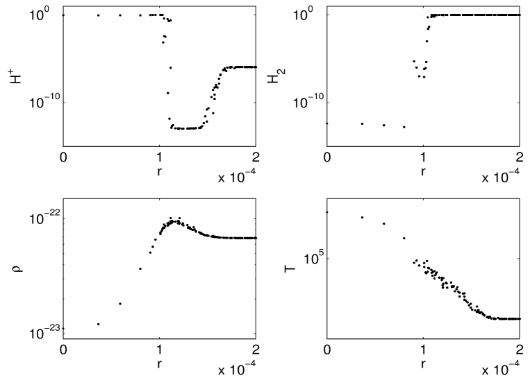
Figure 4: Sedov-Taylor OB-wind test with chemical evolution. Left to right, top to bottom: radial profiles of $\mathrm{H^{+}}$ and $\mathrm{H_{2}}$ mass fractions, $\rho$, and T, at $t=0.5$ Myr. Plotted are all particles within the central 200 pc.

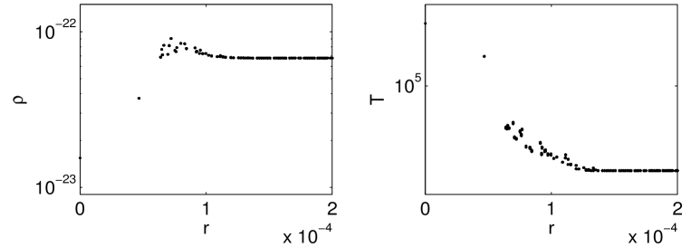
Figure 5: Sedov-taylor OB-wind test without chemical evolution. Left to right: radial profiles of $\rho$ and T, at $t=0.5$ Myr. Plotted are all particles within the central 200 pc.

6 MaNN interfaced with NB-TSPH simulations

To evaluate the performance of MaNN in real large -scale numerical simulations we implemented it in the NB-TSPH code EvoL, and run a “realistic” version of the ideal Sedov-Taylor problem, which is known to be a rather demanding test.

MaNN tracks the evolution of the relative abundances of $\mathrm{H},\mathrm{H^{+}},\mathrm{H_{2}}$ and $\mathrm{e^{-}}$ within each gas particle of the SPH simulation. The MaNN routine is called by each active gas particle during the computation of its radiative cooling (which is in turn obtained from look-up tables, see Merlin & Chiosi 2007,   for details). Since the time interval $\Delta t=10^{4}$ yr in between the initial and the final stage of any model in MaNN is usually smaller than the typical dynamical time step of a gas particle, the routine is called several times until the dynamical time step is covered. If the dynamical time step is not an integer multiple of the MaNN time interval, an interpolation is applied to the results of the last two calls of MaNN. During the whole procedure, all the physical parameters but the afore mentioned relative chemical abundances and the temperature (namely, total density, metallicity and mechanical heating rate) are kept constant.

Due to the detailed description of the chemical properties of each particle, the adiabatic index $\gamma$ in the equation of state governing the gas pressure $P=(\gamma-1)\rho u$ varies as a function of the relative abundances (see Grassi et al. (2010)). This will immediately reflect on the relationship between the internal energy and the temperature, and on the equation of the motion itself. Therefore, we expect an important change in the dynamical evolution of the whole system as compared to the case in which these chemical effects are ignored.

$\begin{array}[]{cc}\includegraphics[width=426.79134pt,height=184.9429pt]{figs/pres.eps}\end{array}$

Figure 6: Sedov-taylor OB-wind test. Pressure field in a central slice of side $l=500$ pc, with (left) and without (right) chemical evolution.

The test run is set up as follows. A uniform grid of $45^{3}$ equal mass gas particles is displaced inside a periodic box of size $l=1$ kpc. The mass of each mass element is $\simeq 10^{4}$ M_⊙, so the initial uniform density is $\rho\simeq 6.78\times 10^{-23}$ g/cm³. The initial temperature is $200$ K. The initial chemical mass fractions of each gaseous element are $[\mathrm{H}^{+}]=10^{-20}$, $[\mathrm{H}_{2}]=0.99$, $\mathrm{H}=1-([\mathrm{H_{2}}]+[\mathrm{H^{+}}])$. These initial conditions resemble a dense interstellar cloud of cold molecular material.

At time $t=0$, the temperature of the central particle is instantaneously raised up to $T=2\times 10^{7}$ K, a temperature similar to that of the gas shocked by the winds ejected by O-B young stars. We name this physical case as the Sedov-Taylor OB-wind. At the same time, the chemical composition of the particle is changed to $[\mathrm{H}_{2}]=10^{-20}$, $[\mathrm{H}^{+}]=0.99$, $\mathrm{H}=1-([\mathrm{H_{2}}]+[\mathrm{H^{+}}])$. The temperature of the central particle is maintained constant, to mimic the continuous energy injection by the central star, and the system is let evolve freely under the action of hydrodynamic interactions and chemical reactions. We also include thermal conduction and radiative cooling that are usually neglected in standard Sedov-Taylor explosion tests (see Merlin et al. 2010,   for more details).

A region of hot material expands in the surroundings of the central particle. This is due to a spurious numerical conduction which, however, causes a numerical smoothing of the initial condition and favors the correct developing of the subsequent evolutionary stages. Then, a shock wave forms and moves outwards radially. Note that the continuous energy release from the central particle and the effect of radiative cooling, almost prevent the inward motion of shocked particles like in standard tests of the Sedov-Taylor explosion.

In Fig. 4 we show the state of the system after $\simeq 0.5$ Myr of evolution. The bottom panels display the density and temperature profiles, and the top panels the abundances of $\mathrm{H}^{+}$ and $\mathrm{H}_{2}$. In the central hot and less dense region, the molecular hydrogen gets completely ionized (the abundance of $\mathrm{H}_{2}$ falls to very low values), due to the high temperatures and low densities. The less dense cavity is surrounded by a layer of over-dense material (the shock layer) which in turn is surrounded by another layer with the initial density. The over-dense front is moving outwards. In the pre-shock region, near the shock layer, the density increase causes the $\mathrm{H^{+}}$ to recombine into neutral hydrogen. These results fairly agree with the theoretical predictions.

To strengthen the above conclusion, we performed another simulation of the Sedov-Taylor OB-wind, in which the effects of the chemical composition and its changes on the gas particles are ignored (by the way this is exactly what is assumed in most if not all the cosmological simulations). In practice, all the gas particles are assumed to be composed of solely neutral H, so that the adiabatic index $\gamma$ is fixed and equal to 5/3. the results are shown in Fig. 5, in which the density and temperature profiles are displayed at the same age of the previous case presented in Fig. 4. Clearly, the dynamical evolution of the system is substantially different. The over-dense front moves at significantly lower speed. In particular, it is clear how the variable chemical composition ensures a higher pressure in the central region containing ionized particles, with respect to the outer region containing molecules. This causes the faster expansion of the central bubble with respect to present case. This is also supported by the pressure fields in the two cases shown in Fig. 6. The left panel shows the pressure field of the first case with evolving chemical composition of the gas particles, whereas the right panel shows the same but for constant chemical composition. The color code shows the value of the pressure in code units. Both pressure fields are measured at the same age of 0.5 Myr and on the surface of an arbitrary plane passing through the center of the computational box. There are a number of interesting features to note: (i) The pressure in the outskirts is lower in the case with chemical evolution, where the adiabatic index is $\gamma=7/5$ for the bi-atomic molecule $\mathrm{H}_{2}$. At the same time, the pressure in the central region of the case with chemical evolution is higher by nearly a factor of two because the number of free particles (or equivalently the internal energy corresponding to a given temperature) is nearly doubled. (ii) The continuous energy release from the central particle, plus the action of the radiative cooling, almost prevent the inward motion of shocked particles (conversely to what happens in the standard Sedov-Taylor explosion test). Instead, they are compressed in a thin layer, which moves outwards under the action of the central source of pressure. For this reason, we are interested in the state of the system shortly after the beginning of the energy release, before the shock layer is pushed too far away from the central region. However, at that moment only a relatively small number of particles have already felt a strong hydrodynamical interaction. This explains the geometrical features that can be seen in Figs. 6. They are due to the initial regular displacement of the particles, whose effects are still to be smeared out by hydrodynamics interactions. Because the detailed chemical treatment implies a larger pressure gradient and, consequently, a faster expansion of the central bubble, after a given $\Delta t$ the simulation without the inclusion of MaNN shows a stronger geometrical spurious asymmetry with respect to the “standard” case: this is simply because it is at a more primordial stage of its evolution.

7 Summary and conclusions

We presented MaNN, an artificial neural network aimed at providing a light and versatile interface between databases of models of the ISM and numerical hydrodynamical codes. In our specific case the ISM models are the outputs of the Robo code developed by Grassi et al. (2010) and the Padova NB-TSPH code EvoL developed by Merlin et al. (2010).

With the aid of Robo we have calculated a large database of ISM models (55000 in total). In these models, given a set of initial conditions, the thermodynamical and chemical evolution of the ISM is followed during a given time interval to get the new physical state of the ISM. A large volume of the hyper-space o f the physical parameters and their initial conditions is explored to get an ensemble of Robo models. For the aims of this first study, the ISM models are calculated switching off the dust, the external heating, and the cosmological evolution. They can be restored at any time.

The above database is fed to MaNN with some simplifications. First of all, a MaNN model is made of two strings (vectors) of quantities: the initial condition for the key parameters (input vector) and the results for the quantities describing the final state after a certain time interval of evolution (output vector). Not necessarily they must be identical in dimension and type of physical quantities. The first step to undertake is to train MaNN to reproduce the results obtained with Robo. The technique in use is the back-propagation algorithm. Once the training stage is completed and the architecture of MaNN is fixed, MaNN is able to mimic the results of Robo with a great degree of accuracy. The great advantage of all of this is that in large cosmological or galactic simulations the thermodynamical and chemical properties of all the gas particles can be determined at each time step with great accuracy in practice at no computational cost.

Finally, we have implemented MaNN into EvoL and run the Sedov-Taylor OB-wind test, i.e. the evolution of a dense and cold molecular cloud during the release of a high amount of energy in its central region. The results are fairly good, showing a nice agreement with the theoretical expectations: while a shock wave develops and moves outwards, a hot and ionized region forms in the central region. Taking into account the detailed chemical evolution greatly affects the thermo-dynamical evolution of the system. Similar effects should be expected in realistic NB-TSPH simulations of cosmological or galactic large scale structures.

In conclusion, MaNN proves to be a practical, easy-to-handle and robust method to include the thermal and chemical properties of the ISM in NB-TSPH simulations.