Bubble nucleation in stout beers

Abstract

Bubble nucleation in weakly supersaturated solutions of carbon dioxide—such as champagne, sparkling wines and carbonated beers—is well understood. Bubbles grow and detach from nucleation sites: gas pockets trapped within hollow cellulose fibres. This mechanism appears not to be active in stout beers that are supersaturated solutions of nitrogen and carbon dioxide. In their canned forms these beers require additional technology (widgets) to release the bubbles which will form the head of the beer. We extend the mathematical model of bubble nucleation in carbonated liquids to the case of two gasses and show that this nucleation mechanism is active in stout beers, though substantially slower than in carbonated beers and confirm this by observation. A rough calculation suggests that despite the slowness of the process, applying a coating of hollow porous fibres to the inside of a can or bottle could be a potential replacement for widgets.

I Introduction

The production of bubbles in weakly supersaturated solutions of carbon dioxide is of great interest to the beverage industry. Such solutions include many soft drinks and beers, as well as sparkling wines and champagne. While it has long been appreciated that spontaneous bubble formation in these liquids is strongly inhibited and thus that bubble formation can only occur at certain nucleation sites [10, 3], it is only comparatively recently that the nature of these sites has been fully elucidated. In a series of papers, Liger-Belair and co-workers demonstrated that the most important nucleation sites are pockets of gas trapped in cellulose fibres [5] (an example of type IV nucleation in the classification of Jones et al. [3]) and developed a mathematical model of the growth and detachment of these bubbles [6], (a complementary model making slighly different assumptions was developed by Uzel et al. [9]).

While most beers are carbonated, there are advantages to using a mixture of nitrogen and carbon dioxide in beers, as is done in a number of stouts. (Hereafter, the term ‘stout’ will be used to refer to a beer containing a mixture of dissolved nitrogen and carbon dioxide.) These advantages include lower acidity in the beer leading to an improved taste; and smaller bubbles giving a creamy mouthfeel and a long lasting head [1, 2]. These beers are interesting scientifically because they show interesting fluid dynamical phenomena such as roll waves [8] and sinking bubbles [11]. Also of scientific interest is the technology used to create the head in the canned products.

Pouring a carbonated beer from the can into a glass is enough to generate the head. This is not the case for stouts. Foaming in canned stouts is promoted by a widget: a hollow ball containing pressurised gas. When the can is opened, the widget depressurises by releasing a gas jet into the beer. The jet breaks up into tiny bubbles which are carried throughout the liquid by the turbulent flow generated by the gas jet and by pouring the beer into a glass. Dissolved gasses diffuse from the liquid into the bubbles which rise to the surface of the beer to form the head.

In this paper we extend the mathematical model of bubble formation in carbonated liquids developed by Liger-Belair et al. [6] to the case of two dissolved gasses and use it to investigate two questions:

• Why do stout beers require widgets? Is the bubbling mechanism described by Liger-Belair et al. completely inactive in stout beers or merely very slow?

• Could an alternative to the widget be developed by coating part of the inside of the can by hollow fibres?

Table 1: Values of parameters used in this work.

Parameter	Value		Reference
$r$	$6.00\times 10^{-6}$	$\,\mathrm{m}$	[6]
$\lambda$	$14.00\times 10^{-6}$	$\,\mathrm{m}$	[6]
$\gamma$	$47.00\times 10^{-3}$	$\,\mathrm{N}\,\mathrm{m}^{-1}$	[1]
$D_{1}$	$1.40\times 10^{-9}$	$\,\mathrm{m}^{2}\,\mathrm{s}^{-1}$
$D_{2}$	$2.00\times 10^{-9}$	$\,\mathrm{m}^{2}\,\mathrm{s}^{-1}$
$H_{1}$	$3.4\times 10^{-4}$	$\,\mathrm{mol}\,\mathrm{m}^{-1}\,\mathrm{N}^{-1}$
$H_{2}$	$6.1\times 10^{-6}$	$\,\mathrm{mol}\,\mathrm{m}^{-1}\,\mathrm{N}^{-1}$
$T$	$293$	$\,\mathrm{K}$
$P_{0}$	$1.00\times 10^{5}$	$\,\mathrm{Pa}$
$P_{1}$	$0.80\times 10^{5}$	$\,\mathrm{Pa}$	[7]
$P_{2}$	$3.00\times 10^{5}$	$\,\mathrm{Pa}$	[7]

II Mathematical Model

In this section we develop a mathematical model of the rate of growth of a gas pocket in a cellulose fibre for the case in which there are two dissolved gasses: nitrogen and carbon dioxide. Once a gas pocket reaches a critical size (when it reaches an opening of the fibre) it rapidly forms a bubble outside the fibre, leaving behind the original gas pocket. Since bubble formation and detachment is much faster than the growth of the gas pocket, the rate at which bubbles are nucleated can be deduced from the rate of growth of the gas pocket [6].

The geometry of a gas pocket in a cellulose fibre is shown in Fig. 1. Dissolved gasses in the fluid diffuse into the bubble through the walls of the cellulose fibre and through the spherical caps at the ends of the gas pocket. The rate at which this occurs is determined by the surface area, the diffusion constant and a diffusion length scale. The diffusion constants used to calculate the fluxes of carbon dioxide and nitrogen through the spherical caps are the diffusion constants in free fluid: $D_{1}$ and $D_{2}$. The relevant diffusion constants for flow through the cellulose walls are $D_{1\perp}$ and $D_{2\perp}$. NMR measurements show that for carbon dioxide $D_{1\perp}\approx 0.2D_{1}$ [4]. We assume the same relationship holds between $D_{2\perp}$ and $D_{2}$. The diffusion lengthscale $\lambda$ was measured experimentally for carbon dioxide [6], again we assume that this value is also valid for nitrogen diffusion.

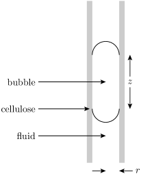
Figure 1: Geometry of a gas pocket trapped in a cellulose fibre.

In this model the rate of change of the numbers of carbon dioxide ($N_{1}^{*}$) and nitrogen ($N_{2}^{*}$) molecules in the gas pocket are given by

$$\dfrac{\text{d}N_{1}^{*}}{\text{d}t^{*}} =4\pi r^{2}D_{1}\dfrac{\Delta c_{1}}{\lambda}+2\pi rzD_{1\perp}\dfrac{\Delta c_{1}}{\lambda},$$ (1)

$$\dfrac{\text{d}N_{2}^{*}}{\text{d}t^{*}} =4\pi r^{2}D_{2}\dfrac{\Delta c_{2}}{\lambda}+2\pi rzD_{2\perp}\dfrac{\Delta c_{2}}{\lambda},$$ (2)

where asterisks indicate dimensional variables that will be non-dimensionalised later.

Using Henry’s law, Laplace’s law and the ideal gas equation:

$$\Delta c_{1} =H_{1}\left(P_{1}-\dfrac{P_{\text{B}}N_{1}^{*}}{N_{1}^{*}+N_{2}^{*}}\right),$$ (3)

$$\Delta c_{2} =H_{2}\left(P_{2}-\dfrac{P_{\text{B}}N_{2}^{*}}{N_{1}^{*}+N_{2}^{*}}\right).$$ (4)

$$P_{\text{B}} =P_{0}+\dfrac{2\gamma}{r},$$ (5)

$$z =\dfrac{\left(N_{1}^{*}+N_{2}^{*}\right)RT}{\pi r^{2}P_{\text{B}}},$$ (6)

where $P_{1}$ is the partial pressure of dissolved carbon dioxide, $P_{2}$ is partial pressure of dissolved nitrogen, $P_{\text{B}}$ is the pressure in the gas pocket given by the Laplace law, $P_{0}$ is atmospheric pressure and $\gamma$ surface tension.

These equations can be non-dimensionalised by using the scales

$$N_{\text{scale}}=\dfrac{2D_{2}}{D_{2\perp}}\dfrac{P_{\text{B}}\pi r^{3}}{RT}\approx 3.22\times 10^{-13}\,\mathrm{mol},$$ (7)

$$t_{\text{scale}}=\dfrac{rP_{\text{B}}\lambda}{2D_{2\perp}H_{2}P_{2}RT}\approx 2.73\,\mathrm{s},$$ (8)

to introduce dimensionless variables $N_{1}$, $N_{2}$ and $t$ (by assumption $D_{2}/D_{2\perp}=D_{1}/D_{1\perp}$). The dimensionless equations are

$$\epsilon\dfrac{\text{d}N_{1}}{\text{d}t} =\left(1+N_{1}+N_{2}\right)\left(1-\dfrac{\alpha_{1}N_{1}}{N_{1}+N_{2}}\right),$$ (9)

$$\dfrac{\text{d}N_{2}}{\text{d}t} =\left(1+N_{1}+N_{2}\right)\left(1-\dfrac{\alpha_{2}N_{2}}{N_{1}+N_{2}}\right).$$ (10)

Using values typical of stouts, given in Table 1, the dimensionless parameters are

$$\epsilon=\dfrac{D_{2}H_{2}P_{2}}{D_{1}H_{1}P_{1}}\approx 0.096,$$ (11)

$$\alpha_{1}=\dfrac{P_{\text{B}}}{P_{1}}\approx 1.45,$$ (12)

$$\alpha_{2}=\dfrac{P_{\text{B}}}{P_{2}}\approx 0.39.$$ (13)

III Asymptotic Solution

Equations 9 and 10 cannot be solved directly. They can, however, be solved in two asymptotic limits: $\epsilon\ll 1$ and $N_{1}+N_{2}\gg 1$. The former limit does not produce particularly accurate results but the analysis of this limit helps us to interpret the results from taking the second asymptotic limit. The results from taking the second asymptotic limit are more accurate but harder to understand intuitively.

III.1 First asymptotic limit: $\boldsymbol{\epsilon\ll 1}$

Taking the limit in which the small parameter $\epsilon\approx 0.1$ is zero, equation 9 becomes an algebraic equation

$$0=1-\dfrac{\alpha_{1}N_{1}}{N_{1}+N_{2}},$$ (14)

which can be substituted into equation 10

$$\dfrac{\text{d}N_{2}}{\text{d}t}=\dfrac{\alpha_{1}+\alpha_{2}-\alpha_{1}\alpha_{2}}{\alpha_{1}-1}N_{2}+\dfrac{\alpha_{1}+\alpha_{2}-\alpha_{1}\alpha_{2}}{\alpha_{1}}.$$ (15)

This equation is solved by

$$N_{2}=A\exp\!\left(\dfrac{t}{\tau}\right)-\dfrac{\alpha_{1}+\alpha_{2}-\alpha_{1}\alpha_{2}}{\alpha_{1}},$$ (16)

where $A$ is a constant of integration and $\tau$ a dimensionless time constant describing the timescale of growth of the gas pocket in this approximation

$$\tau=\dfrac{\alpha_{1}-1}{\alpha_{1}+\alpha_{2}-\alpha_{1}\alpha_{2}}\approx 0.35,$$ (17)

$$\tau t_{\text{scale}}=0.954\,\mathrm{s}.$$ (18)

Physically this approximation corresponds to assuming that diffusion of carbon dioxide is infinitely fast, and thus the partial pressure of carbon dioxide in the gas pocket is always equal to the partial pressure of carbon dioxide in solution. Obviously this approximation is only valid if the partial pressure of carbon dioxide is less than the gas pocket pressure, otherwise equation 14 has no physical solutions. Note that this approximation will underestimate $\tau$ since it assumes carbon dioxide diffusion is infinitely fast.

III.2 Second asymptotic limit: $\boldsymbol{N_{1}+N_{2}\gg 1}$

Table 2: Numerical values of the parameters in equations 21 and 22.

Parameter	Value
$a_{11}$	0.	989
$a_{12}$	0.	836
$a_{21}$	–0.	145
$a_{22}$	0.	548
$\tau_{1}$	0.	161
$\tau_{2}$	0.	468
$\tau_{1}t_{\text{scale}}$	0.	439 s
$\tau_{2}t_{\text{scale}}$	1.	278 s

In the limit $N_{1}+N_{2}\gg 1$ equations 9 and 10 become

$$\dfrac{\text{d}N_{1}}{\text{d}t} =-\dfrac{\alpha_{1}-1}{\epsilon}N_{1}+\dfrac{N_{2}}{\epsilon},$$ (19)

$$\dfrac{\text{d}N_{2}}{\text{d}t} =N_{1}+\left(1-\alpha_{2}\right)N_{2}.$$ (20)

These equations have two independent solutions

$$N_{1}=Aa_{11}\exp\!\left(-\dfrac{t}{\tau_{1}}\right),\quad N_{2}=Aa_{21}\exp\!\left(-\dfrac{t}{\tau_{1}}\right),$$ (21)

and

$$N_{1}=Ba_{12}\exp\!\left(\dfrac{t}{\tau_{2}}\right),\quad N_{2}=Ba_{22}\exp\!\left(\dfrac{t}{\tau_{2}}\right),$$ (22)

where $A$ and $B$ can be chosen independently to satisfy initial conditions. The numerical values of the other parameters are given in Table 2.

The analysis of the $\epsilon\ll 1$ case allows us to interpret these two solutions. The first solution, equation 21, decays exponentially with a small timescale. This corresponds to the rapid establishment of the (dynamic) equilibrium concentrations (or partial pressures) of CO₂ and N₂ within the gas pocket (assumed instantaneous in the previous analysis). The second solution, equation 22, shows exponential growth with a longer timescale. This describes the steady state growth of the gas pocket at a fixed concentration ratio of CO₂ to N₂. The timescale of this process describes the timescale of bubble production. This analysis produces a longer estimate of that timescale than the previous analysis. This is because, previously, diffusion of CO₂ was assumed to be instantaneous. As the numerical results described in the next section show, the $\epsilon\ll 1$ limit underestimates the correct timescale, while the $N_{1}+N_{2}\gg 1$ analysis gives a good estimate.

IV Numerical Solution

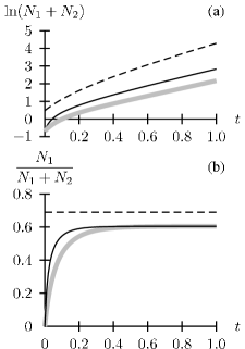
Figure 2: Results of the numerical solution of equations 9 and 10. The black line shows the numerical solution, the grey line shows the $N_{1}+N_{2}\gg 1$ limit, and the dashed black line shows the $\epsilon\ll 1$ limit. (a) Rate of growth of the gas pocket. (b) Evolution of the concentration of CO₂ in the gas pocket.

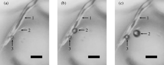
Figure 3: Bubble nucleation in stout from a cellulose fibre taken from a coffee filter. The scalebar is $50\,\upmu\text{m}$ in each figure. The arrows show: 1 a gas pocket in the fibre which nucleates a bubble; 2 the bubble fed by gas from pocket 1; 3 a bubble nucleated on the outside of the fibre. (a) The air pocket (1) has reached maximum size. (b) The air pocket (1) has created bubble (2). (c) Bubble (2) has visibly detached from the fibre, air pocket (1) is starting to refill with gas. (a), (b) and (c) are frames from a movie. (b) is $80\,\mathrm{ms}$ after (a), (c) is $520\,\mathrm{ms}$ after (a).

A full solution of the dimensionless equations can be obtained by numerical integration. A fourth order Runge-Kutta scheme with a timestep of $10^{-3}$ was used to solve equations 9 and 10 with initial conditions $N_{1}=0$, $N_{2}=0.5$. The differential equations were solved over the interval $0<t<10$. The result for $N=N_{1}+N_{2}$ for $5<t<10$ were fitted to an exponential curve giving a dimensionless bubble growth timescale of $\tau=0.47$ corresponding to a dimensional timescale of $\tau t_{\text{scale}}=1.28\,\mathrm{s}$, in agreement with that predicted from the analysis of the $N_{1}+N_{2}\gg 1$ case. This can be compared with the value for carbonated liquids at the same total pressure: $0.079\,\mathrm{s}$. Fig. 2 shows the results of the numerical simulations over the interval $0<t<1$.

In conclusion, these analytic and numerical results suggest that the mechanism of bubble formation described by Liger-Belair et al. is potentially active in stout beers but acts much more slowly than in carbonated drinks.

V Experimental Confirmation

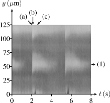
Figure 4: Growth of the gas pocket. This figure shows the growth of the gas pocket within the cellulose fibre shown in Fig. 3. As in Fig. 3 dark colours correspond to gas and light colours to liquid. The columns of pixels from the frames corresponding to parts (a), (b) and (c) of Fig. 3 are indicated. The location of the gas pocket indicated by a (1) in Fig. 3 is shown.

To confirm experimentally that cellulose fibres could nucleate bubbles in stout beer, we observed a canned draught stout in contact with cellulose fibres (taken from a coffee filter). Before opening the can, we made a small hole in the can to slowly degass the widget. This prevented it from foaming, which would have removed the dissolved gasses from solution. Using a microscope we observed that bubbles were indeed nucleated from the cellulose fibres but at a relatively slow rate. Fig. 3 shows bubbles nucleated by a gas pocket: the three parts of Fig. 3 are frames taken from a movie.

Fig. 4 shows the growth of the gas pocket shown in Fig. 3. The figure was constructed from the same movie of the bubbling process used for Fig. 3. Two hundred frames, corresponding to $8\,\mathrm{s}$ were extracted from the movie and rotated so that the fibre shown in Fig. 3 was vertical. From each frame the same column of pixels, passing through the centre of the fibre, was extracted and those columns placed side by side to construct a new figure: Fig. 4. This figure shows the evolution of the gas pocket: its slow growth (as predicted by the model) and then its rapid loss of gas to form an external bubble (as assumed by the model).

VI Widget Alternatives

The model developed above allows us to investigate the feasibility of an alternative foaming strategy for stout beers in cans and bottles in which a coating of hydrophobic fibres on the inside of the can is used to promote foaming. A typical pouring time for a stout beer is $30\,\mathrm{s}$. In this time about $10^{8}$ postcritical nuclei must be released. A single fibre produces one bubble every $1.28\,\mathrm{s}$. Therefore about $4.3\times 10^{6}$ fibres are needed. If each fibre occupies a surface of area $\lambda^{2}$ then the total area that must be occupied by fibres is $8.3\times 10^{-4}\,\mathrm{m}^{2}$ equivalent to a square with edge length $2.9\,\mathrm{cm}$. This indicates that such an approach may be possible.

VII Conclusions

A model of bubble formation in carbonated liquids has been extended to the case of liquids containing both dissolved nitrogen and carbon dioxide. Taking values typical of stout beers shows that bubble formation by this mechanism does occur but at a substantially slower rate. This is consistent with the observation that widgets are needed to promote foaming in canned stouts. The possibility of replacing widgets with an array of hollow fibre nucleation sites was investigated and shown to be potentially feasible.

- [1] C. W. Bamforth. The relative significance of physics and chemistry for beer foam excellence: Theory and practice. Journal of the Institute of Brewing, 110:259–266, 2004.
- [2] M. Denny. Froth!: the science of beer. The Johns Hopkins University Press, Baltimore, 2009. Pages 129–131.
- [3] S. F. Jones, G. M. Evans, and K. P. Galvin. The cycle of bubble production from a gas cavity in a supersaturated solution. Adv. Colloid Interface Sci., 80:51–84, 1999.
- [4] G. Liger-Belair, D. Topgaard, C. Voisin, and P. Jeandet. Is the wall of a cellulose fiber saturated with liquid whether or not permeable with CO2 dissolved molecules? Application to bubble nucleation in champagne wines. Langmuir, 20:4132–4138, 2004.
- [5] G. Liger-Belair, M. Vignes-Adler, C. Voisin, B. Robillard, and P. Jeandet. Kinetics of gas discharging in a glass of champagne: The role of nucleation sites. Langmuir, 18:1294–1301, 2002.
- [6] G. Liger-Belair, C. Voisin, and P. Jeandet. Modeling nonclassical heterogeneous bubble nucleation from cellulose fibers: Application to bubbling in carbonated beverages. J. Phys. Chem. B, 109:14573–14580, 2005.
- [7] O. A. Power, W. T. Lee, A. C. Fowler, P. J. Dellar, L. W. Schwartz, S. Lukaschuk, G. Lessells, A. F. Hegarty, M. O’Sullivan, and Y. Liu. The initiation of Guinness. In S. B. G. O’Brien, M. O’Sullivan, P. Hanrahan, W. T. Lee, J. Mason, J. Charpin, M. Robinson, and A. Korobeinikov, editors, Proceedings of the Seventieth European Study Group with Industry, pages 141–182, 2009.
- [8] M. Robinson, A. C. Fowler, A. J. Alexander, and S. B. G. O’Brien. Waves in Guinness. Phys. Fluids, 20:067101, 2008.
- [9] S. Uzel, M. A. Chappell, and S. J. Payne. Modeling the cycles of growth and detachment of bubbles in carbonated beverages. J. Phys. Chem. B, 110:7579–7586, 2006.
- [10] J. Walker. Reflections on the rising bubbles in a bottle of beer. Am. Sci., 245:124–132, 1981.
- [11] Y. Zhang and Z. Xu. “Fizzics” of bubble growth in beer and champagne. Elements, 4:47–49, 2008.