On the $\text{AdS}_{5}/\text{CFT}_{4}$ TBA and its analytic properties

Abstract

The thermodynamic Bethe Ansatz equations arising in the context of the $\text{AdS}_{5}/\text{CFT}_{4}$ correspondence exhibit an important difference with respect to their analogues in relativistic integrable quantum field theories: their solutions (the Y functions) are not meromorphic functions of the rapidity, but live on a complicated Riemann surface with an infinite number of branch points and therefore enjoy a new kind of extended Y-system. In this paper we review the analytic properties of the TBA solutions, and present new information coming from their numerical study. An identity allowing to simplify the equations and the numerical implementation is presented, together with various plots which highlight the analytic structure of the Y functions.

1 Introduction

In 1997 Maldacena [1] (see also [2]) conjectured a correspondence between gravity and conformal gauge theory of strong/weak type and, in particular, the duality $\text{AdS}_{5}/\text{CFT}_{4}$ between the supersymmetric string theory of type IIB on a curved space $\text{AdS}_{5}\times\text{S}^{5}$ and ${\cal N}=4$ super Yang-Mills (SYM).

A turning point for the study of the correspondence $\text{AdS}_{5}/\text{CFT}_{4}$ was the discovery of integrability in the ’t Hooft limit, both for the string theory [3, 4] and the conformal field theory $\text{CFT}_{4}$ [5]. The ’t Hooft planar limit is defined by the scaling of the colour number $N\rightarrow\infty$ and the SYM coupling $g_{YM}\rightarrow 0$ while keeping the coupling $Ng_{YM}^{2}=\lambda=4\pi^{2}g^{2}$ finite, so that $g$ is proportional to the string tension. In this limit only planar Feynman diagrams survive [6].

The Bethe Ansatz (BA) method was originally introduced by H. Bethe [7] in 1931 to study a one-dimensional quantum system of spin $1/2$ and determine its eigenvalues and eigenstates. This system is also known as the Heisenberg XXX model and, since the scattering of the possible excitations can always be factored in terms of two-body amplitudes, it has the feature of being integrable.

In the ${\cal N}=4$ SYM context, a set of Bethe Ansatz-like equations were formulated by Beisert and Staudacher  [8] (see also  [9]) as a useful tool to compute the anomalous dimensions of SYM composite single trace operators or the energy of the quantum states of the string. However, the equations emerging in this framework do not take into account the wrapping effects due to the finite number of elementary operators in the trace [10, 11]. Therefore, the Beisert-Staudacher’s equations lead to exact results only for asymptotically long operators and are the analogue of the Bethe-Yang equations for scattering models describing the quantisation of momenta for a finite number of interacting particles living on a ring with very large circumference [12, 13].

A first important step towards the partial solution of the wrapping problem was made in [14]. Adapting the formulas for the finite-size Lüscher corrections [15, 16] to the $\text{AdS}_{5}/\text{CFT}_{4}$ context, Bajnok and Janik were able to predict the four loop contribution to the Konishi operator. The result was readily confirmed by the perturbative calculations of [17]. The ideas proposed in [14] can be applied to higher perturbative orders and twists [18, 19] but technical complications increase dramatically with the loop order and, through this approach, exact all-loop results are probably out of reach.

An alternative tool to find the finite-size corrections to the ground state energy in 2D integrable models was proposed many years ago by Aliosha Zamolodchikov [20] modifying the thermodynamic Bethe Ansatz (TBA) whose original formulation traces back to Yang and Yang [21]. The TBA method leads to a set of coupled non-linear integral equations governing, as the parameters of the model are changed, the ground state energy of the theory on a cylinder exactly and non-perturbatively.

As discussed in [22], consider a two-dimensional euclidean quantum field theory defined on a torus with circumferences $R$ and $L$, as shown in Figure 1.

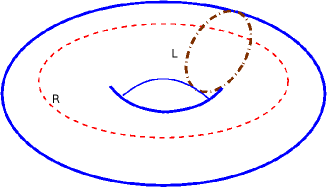
Figure 1: The two hamiltonian descriptions of a 2D euclidean model.

The quantization of this theory is equivalently obtained by considering two alternative hamiltonian schemes. In the direct scheme the system is quantised along the direction $L$ and the hamiltonian ${\cal H}_{L}$ propagates the states in the time direction $R$. In the mirror scheme the system is described by the hamiltonian ${\cal H}_{R}$ and the roles of $L$ and $R$ are swapped. The two descriptions lead to the same partition function

(1) $$Z(R,L)=\text{Tr}(e^{-R{\cal H}_{L}})=\text{Tr}(e^{-L{\cal H}_{R}}).$$

Sending $R\rightarrow\infty$, in the direct description of the theory the partition function is dominated by the smallest eigenvalue $E_{0}(L)$ of ${\cal H}_{L}$:

(2) $$Z(R,L)=\text{Tr}(e^{-R{\cal H}_{L}})\sim e^{-RE_{0}(L)}.$$

While, in the mirror description, the $R\rightarrow\infty$ limit corresponds to the thermodynamics of a one-dimensional quantum system with hamiltonian ${\cal H}_{R}$ defined on a volume $R$ at temperature $T=\frac{1}{L}$. In this picture, the partition function becomes

(3) $$Z(R,L)=\text{Tr}(e^{-L{\cal H}_{R}})\sim e^{-LRf(L)},$$

where $f(L)$ is the free energy per unit length at equilibrium. Comparing (2) with (3) we see that the ground state energy of the direct theory is related to the equilibrium free energy of the mirror theory:

(4) $$E_{0}(L)=Lf(L).$$

Starting from the Bethe-Yang equations for the mirror theory, $f(L)$ can be found [20] adapting the method proposed in [21] for a one-dimensional system of bosons with repulsive delta-function interaction. As a result of the TBA procedure, the exact finite-size ground state energy $E_{0}(L)$ is written in terms of the pseudoenergies $\varepsilon_{a}$, solutions to a set of coupled non-linear integral equations. In [23, 24, 25, 26] the method was extended to excited states and an alternative but equivalent approach was proposed in [27, 28, 29] (This alternative tool has also been used in the $\text{AdS}/\text{CFT}$ setup in [30, 31, 32, 33]). Starting from the mirror version of the Beisert-Staudacher’s equations [34, 35], the ground state TBA equations were independently derived in [36, 37, 38] and precise conjectures for particular excited state sectors were made in [39, 37, 40].

Because the equations for excited states are expected to be the analytic continuation of the ground state equations [24, 25], the understanding of the analytic structure of the TBA system is essential in the attempt to establish the results of [39, 37, 40] rigorously and to generalize them to other sectors of the theory.

The rest of this paper is organised as follows. Section 2 contains the TBA equations of [36, 37, 38]. The pseudoenergies have an infinite number of square root branch cuts and, basically, the $\text{AdS}_{5}/\text{CFT}_{4}$ TBA equations are equivalent to a set of functional relations containing also information on the discontinuities across the cuts [41]: the extended Y-systems described in Section 3. Following [41], Section 4 discusses briefly the interpretation of the TBA as dispersion relations and, using byproduct identities of [41], a variant of the TBA equations more suitable for numerical integration is proposed in Section 3. Sections 6-8 contain our preliminary numerical results for the ground state energy and a study of the pseudoenergies in the complex rapidity plane. Finally, Section 9 contains our conclusions and the S-matrix elements corresponding to the TBA kernels are listed in Appendix A.

2 The TBA equations

The TBA equations with arbitrary chemical potentials $\{\mu_{a}\}$ are [36, 37, 38] :

(5) $$\begin{split}\varepsilon_{Q}(u)&=\mu_{Q}+L\,\tilde{E}_{Q}(u)-\sum_{Q^{\prime}}L_{Q^{\prime}}*\phi^{\Sigma}_{Q^{\prime}Q}(u)\\ &+\sum_{\alpha}{\Big{(}}\sum_{M}L^{(\alpha)}_{(v|M)}*\phi_{(v|M),Q}(u)+L^{(\alpha)}_{y}{*_{\bar{\gamma}_{\sf o}}}\;\phi_{y,Q}(u){\Big{)}},\\ \end{split}$$

(6) $$\begin{split}\varepsilon^{(\alpha)}_{(v|K)}(u)&=\mu_{(v|K)}^{(\alpha)}-\sum_{Q}L_{Q}*\phi_{Q,(v|K)}(u)+\sum_{M}L^{(\alpha)}_{(v|M)}*\phi_{MK}(u)+L^{(\alpha)}_{y}{*_{\bar{\gamma}_{\sf o}}}\;\phi_{K}(u),\end{split}$$

(7) $$\begin{split}\varepsilon^{(\alpha)}_{(w|K)}(u)&=\mu_{(w|K)}^{(\alpha)}+\sum_{M}L^{(\alpha)}_{(w|M)}*\phi_{MK}(u)+L^{(\alpha)}_{y}{*_{\bar{\gamma}_{\sf o}}}\;\phi_{K}(u),\end{split}$$

(8) $$\begin{split}\varepsilon_{y}^{(\alpha)}(u)&=\mu_{y}^{(\alpha)}-\sum_{Q}L_{Q}*\phi_{Q,y}(u)+\sum_{M}(L^{(\alpha)}_{(v|M)}-L^{(\alpha)}_{(w|M)})*\phi_{M}(u),\end{split}$$

where $L\in{\mathbb{N}}$ is the inverse of the temperature, while the sums are taken as $\sum_{{\alpha}=1,2}$, $\sum_{K=1}^{\infty}$, with

$$\tilde{E}_{Q}(u)=\ln{\frac{x(u-i{\textstyle\frac{Q}{g}})}{x(u+i{\textstyle\frac{Q}{g}})}},\;\;x(u)=\left(\frac{u}{2}-i\sqrt{1-\frac{u^{2}}{4}}\right),\;\;\text{Im}(x)<0,$$

(9) $$Y_{a}(u)=e^{\varepsilon_{a}(u)},~{}~{}L_{a}(u)=\ln(1+1/Y_{a}(u)),$$

and the symbols ‘$*$’ and ‘$*_{\gamma}$’ denote the convolutions

$${\cal F}*\phi(u)=\int_{{\mathbb{R}}}dz\;{\cal F}(z)\,\phi(z,u),~{}~{}{\cal F}*_{\gamma}\phi(u)=\oint_{\gamma}dz\;{\cal F}(z)\,\phi(z,u).$$

The kernels are derived from the matrix elements $S_{ab}(z,u)$ listed in Appendix A using the relation: $\phi_{ab}(z,u)=\frac{1}{2\pi i}\frac{d}{dz}\ln S_{ab}(z,u)$. $\phi^{\Sigma}_{Q^{\prime}Q}$ in (5) can be written as:

(10) $$\phi^{\Sigma}_{Q^{\prime}Q}(z,u)=-\phi_{Q^{\prime}Q}(z-u)-2K^{\Sigma}_{Q^{\prime}Q}(z,u),$$

with [36, 37, 38, 42, 43, 44, 45, 41]

(11) $$\phi_{Q^{\prime}Q}(u)=\frac{1}{2\pi i}\frac{d}{du}\ln S_{Q^{\prime}Q}(u),~{}K_{\Gamma}^{[2]}(z-t)=\frac{1}{2\pi i}\frac{d}{dz}\ln\frac{\Gamma(1-ig(z-t)/2)}{\Gamma(1+ig(z-t)/2)},$$

(12) $$K^{\Sigma}_{Q^{\prime}Q}(z,u)=\frac{1}{2\pi i}\frac{d}{dz}{\ln\Sigma}_{Q^{\prime}Q}(z,u)=\oint_{\bar{\gamma}_{\sf x}}ds\;\phi_{Q^{\prime},y}(z,s)\oint_{\bar{\gamma}_{\sf x}}dt\;K_{\Gamma}^{\left[2\right]}(s-t)\phi_{y,Q}(t,u).$$

The contours of integration $\bar{\gamma}_{\sf o}$ and $\bar{\gamma}_{\sf x}$ are represented in Figure 3 and Figure 3, respectively.

Figure 2: The contour $\bar{\gamma}_{\sf o}$.

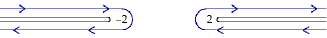
Figure 3: The contour $\bar{\gamma}_{\sf x}$.

The functions $Y_{a}(u)=e^{\varepsilon_{a}(u)}$ solutions of equations (5-8) live on branched coverings of the complex u-plane with an infinite number of square root singularities $u=\{\pm 2+im/g\}$ with $m\in{\mathbb{Z}}$. For the mirror $\text{AdS}_{5}/\text{CFT}_{4}$ theory under consideration -on the sheet containing the physical values of the Ys- all the cuts are conventionally set parallel to the real axis and external to the strip $|\text{Re}(u)|<2$. This will be referred to as the reference or first sheet. Table 1 shows the location of the square branch points for the various Ys.

Function	Singularity positions
$Y^{(\alpha)}_{y}(u)$	$u=\pm 2+i\frac{2J}{g}$,	$J=0,\pm 1,\pm 2,\dots$
$Y^{(\alpha)}_{(w|M)}(u)$
$Y^{(\alpha)}_{(v|M)}(u)$	$u=\pm 2+i\frac{J}{g}$,	$J=\pm M,\pm(M+2),\pm(M+4),\dots$
$Y_{M}(u)$

Table 1: Square root branch points for the Y functions.

Finally, we shall denote with $Y^{(\alpha)}_{(y|-)}(u)$ (or simply $Y^{(\alpha)}_{y}(u)$) the first sheet determination of $Y^{(\alpha)}_{y}$ and with $Y^{(\alpha)}_{(y|+)}(u)=Y^{(\alpha)}_{y}(u_{*})$ its second sheet evaluation obtained by analytically continuing $u$ to $u_{*}$ through the branch cut $u\in(-\infty,-2)$ (see, Figure 5).

3 The extended Y-system

The Y-system [46, 47, 48, 49] for $\text{AdS}_{5}/\text{CFT}_{4}$ was conjectured in [39], rigorously derived in [36, 37, 38] and it is associated to the diagram represented in Figure 4. Setting

(13) $$\begin{split}\Lambda_{Q}&=\prod_{Q^{\prime}}e^{\mu_{Q^{\prime}}\;C_{Q^{\prime}Q}},~{}~{}~{}\Lambda^{(\alpha)}_{(y|-)}=e^{2\mu_{y}^{(\alpha)}-\mu_{(v|1)}^{(\alpha)}+\mu_{(w|1)}^{(\alpha)}},\\ \Lambda^{(\alpha)}_{(w|K)}&=\prod_{M}e^{\mu_{(w|M)}^{(\alpha)}\;C_{MK}},~{}~{}~{}\Lambda^{(\alpha)}_{(v|K)}=\prod_{M}e^{\mu_{(v|M)}^{(\alpha)}\;C_{MK}},\end{split}$$

with $C_{MN}=2\delta_{M,N}-A_{MN}$, $A_{1,M}=\delta_{2,M}$, $A_{NM}=\delta_{M,N+1}+\delta_{M,N-1}$ and $A_{MN}=A_{NM}$, the Y-system with arbitrary chemical potentials is:

(14) $$Y_{Q}(u-{\textstyle\frac{i}{g}})Y_{Q}(u+{\textstyle\frac{i}{g}})=\Lambda_{Q}\prod_{Q^{\prime}}\left(1+Y_{Q^{\prime}}(u)\right)^{A_{QQ^{\prime}}}\prod_{\alpha}\frac{\left(1+\frac{1}{Y_{(v|Q-1)}^{(\alpha)}(u)}\right)^{\delta_{Q,1}-1}}{{\left(1+\frac{1}{Y_{(y|-)}^{(\alpha)}(u)}\right)^{\delta_{Q,1}}}},$$

(15) $$Y_{(y|-)}^{(\alpha)}(u+{\textstyle\frac{i}{g}})Y_{(y|-)}^{(\alpha)}(u-{\textstyle\frac{i}{g}})=\Lambda^{(\alpha)}_{(y|-)}\frac{\left(1+Y_{(v|1)}^{(\alpha)}(u)\right)}{\left(1+Y_{(w|1)}^{(\alpha)}(u)\right)}\frac{1}{\left(1+\frac{1}{Y_{1}(u)}\right)},$$

(16) $$Y_{(w|M)}^{(\alpha)}(u+{\textstyle\frac{i}{g}})Y_{(w|M)}^{(\alpha)}(u-{\textstyle\frac{i}{g}})=\Lambda^{(\alpha)}_{(w|M)}\prod_{N}\left(1+Y_{(w|N)}^{(\alpha)}(u)\right)^{A_{MN}}\left[\frac{\left(1+\frac{1}{Y^{(\alpha)}_{(y|-)}(u)}\right)}{\left(1+\frac{1}{Y^{(\alpha)}_{(y|+)}(u)}\right)}\right]^{\delta_{M,1}},$$

(17) $$Y_{(v|M)}^{(\alpha)}(u+{\textstyle\frac{i}{g}})Y_{(v|M)}^{(\alpha)}(u-{\textstyle\frac{i}{g}})=\Lambda^{(\alpha)}_{(v|M)}\frac{\prod_{N}\left(1+Y_{(v|N)}^{(\alpha)}(u)\right)^{A_{MN}}}{\left(1+\frac{1}{Y_{M+1}(u)}\right)}\left[\frac{\left(1+Y^{(\alpha)}_{(y|-)}(u)\right)}{\left(1+Y^{(\alpha)}_{(y|+)}(u)\right)}\right]^{\delta_{M,1}}.$$

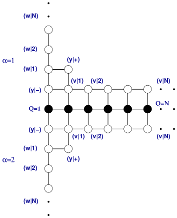
Figure 4: The Y-system diagram corresponding to the $\text{AdS}_{5}/\text{CFT}_{4}$ TBA equations.

In relativistic integrable models the Y functions are in general meromorphic in the rapidity $u$ with zeroes and poles both linked to $1+Y_{a}$ zeroes through the Y-system. Unfortunately, the situation for $\text{AdS}_{5}/\text{CFT}_{4}$ is further complicated by the presence of square root branch cuts inside and at the border of the fundamental strip $|\text{Im}(u)|\leq 1/g$. According to the known Y $\rightarrow$ TBA transformation procedures, together with the asymptotics of the Y functions this extra information on their analytic behaviour should be independently supplied.

However, the crucial discontinuity information is stored into functions which depend non-locally on the TBA pseudoenergies [38, 41] and thus on the particular excited state under consideration.

The main objective of the paper [41] was to show how this problem can be overcome and that all the necessary analytic information can compactly be encoded in the basic Y-system (14-17) extended by the following set of local and state-independent discontinuity relations. Setting

(18) $$\Delta(u)=\left[\ln Y_{1}(u)\right]_{+1},$$

then $\Delta$ is the function introduced in [38] and the discontinuity relations are:

(19) $$\left[\Delta\right]_{\pm 2N}=\mp\sum_{\alpha=1,2}{\biggl{(}}\biggl{[}\ln\biggl{(}1+\frac{1}{Y_{(y|\mp)}^{(\alpha)}}\biggr{)}\biggr{]}_{\pm 2N}+\sum_{M=1}^{N}\biggl{[}\ln\biggl{(}1+\frac{1}{Y^{(\alpha)}_{(v|M)}}\biggr{)}\biggr{]}_{\pm(2N-M)}+\ln{\biggl{(}\frac{Y_{(y|-)}^{(\alpha)}}{Y_{(y|+)}^{(\alpha)}}\biggl{)}}\biggl{)},$$

(20) $$\biggl{[}\ln\biggl{(}\frac{Y^{(\alpha)}_{(y|-)}}{Y^{(\alpha)}_{(y|+)}}\biggl{)}\biggr{]}_{\pm 2N}=-\sum_{Q=1}^{N}\left[\ln\left(1+\frac{1}{Y_{Q}}\right)\right]_{\pm(2N-Q)},$$

with $N=1,2,\dots,\infty$ and

(21) $$\left[\ln{Y^{(\alpha)}_{(w|1)}}\right]_{\pm 1}=\ln\biggl{(}\frac{1+1/Y_{(y|-)}^{(\alpha)}}{1+1/Y_{(y|+)}^{(\alpha)}}\biggl{)},~{}~{}~{}~{}\left[\ln{Y^{(\alpha)}_{(v|1)}}\right]_{\pm 1}=\ln\biggl{(}\frac{1+Y_{(y|-)}^{(\alpha)}}{1+Y_{(y|+)}^{(\alpha)}}\biggl{)},$$

where the symbol $[f]_{Z}$ with $Z\in{\mathbb{Z}}$ denotes the discontinuity of $f(z)$

(22) $$\left[f\right]_{Z}=\lim_{\epsilon\rightarrow 0^{+}}f(u+iZ/g+i\epsilon)-f(u+iZ/g-i\epsilon),$$

on the semi-infinite segments described by $z=u+iZ/g$ with $u\in(-\infty,-2)\cup(2,\infty)$ and the function $\left[f\right(u)]_{Z}$ is the analytic extension of the discontinuity (22) to generic complex values of $u$. Finally, $\Delta(u)$ has an additional constant discontinuity running along the imaginary axis:

(23) $$\Delta(iv+\epsilon)-\Delta(iv-\epsilon)=i2L\pi,~{}(v\in{\mathbb{R}}).$$

In conclusion, while the Y functions are defined on an infinite sheeted Riemann surface, the basic Y-system (14-17) connects points lying on a single reference sheet missing a huge amount of analyticity data. To recover this information it is necessary to extend (14-17) by including relations among different Riemann sheets. This is precisely the information contained in discontinuity relations and, to highlight this fact, one could write equations (18-21) in a more explicit functional form involving points from different sheets. For example (cf (21)):

(24) $$\frac{Y^{(\alpha)}_{(w|1)}(u\pm{\textstyle\frac{i}{g}})}{Y^{(\alpha)}_{(w|1)}(u_{*}\pm{\textstyle\frac{i}{g}})}=\biggl{(}\frac{1+1/Y_{(y|-)}^{(\alpha)}(u)}{1+1/Y_{(y|+)}^{(\alpha)}(u)}\biggl{)},~{}~{}~{}~{}\frac{Y^{(\alpha)}_{(v|1)}(u\pm{\textstyle\frac{i}{g}})}{Y^{(\alpha)}_{(v|1)}(u_{*}\pm{\textstyle\frac{i}{g}})}=\biggl{(}\frac{1+Y_{(y|-)}^{(\alpha)}(u)}{1+Y_{(y|+)}^{(\alpha)}(u)}\biggl{)},$$

where $u_{*}$ is the second sheet image of $u$ reached by analytic continuation through the branch cut $u\in(-\infty,-2)$ (see, Figure 5).

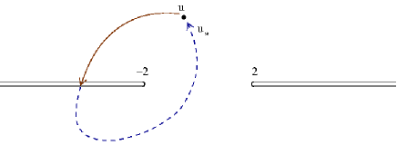
Figure 5: The second sheet image $u_{*}$ of $u$.

4 TBA equations as dispersion relations

As already mentioned in the introductory section, contrary to the more studied relativistic invariant cases, the transformation from Y-system to TBA equations is by no means straightforward since the local form of the $\text{AdS}_{5}/\text{CFT}_{4}$-related Y-system (14-17) alone does not contain information on the branch points and it is almost totally insensitive to the precise form of the dressing factor $\Sigma_{Q^{\prime}Q}$ defined through equation (12). The purpose of this section is to give some hints on why the extension of the basic Y-system by the discontinuity relations (19-21) resolves this problem completely. The interested reader is addressed to [41] for a more complete discussion on this important issue. Consider the following equation directly descending from (8):

(25) $$\ln\left(Y^{(\alpha)}_{(y|-)}(u)/Y^{(\alpha)}_{(y|+)}(u)\right)=-\sum_{Q}\int_{{\mathbb{R}}}dz\,L_{Q}(z)(K(u-iQ/g,z)-K(u+iQ/g,z)),$$

where

(26) $$K(z,u)=\frac{\sqrt{4-u^{2}}}{2\pi i\sqrt{4-z^{2}}}\frac{1}{z-u}.$$

Then, it can be shown that the functional relation (20) on the discontinuities

(27) $$\left[\ln\left(Y^{(\alpha)}_{(y|-)}/Y^{(\alpha)}_{(y|+)}\right)\right]_{\pm 2N}=-\sum_{Q=1}^{N}[L_{Q}]_{\pm(2N-Q)},$$

combined with some more general analyticity information, is equivalent to (25). This result comes from the observation that the quantity:

$$\frac{\ln\left(Y^{(\alpha)}_{(y|-)}(u)/Y^{(\alpha)}_{(y|+)}(u)\right)}{\sqrt{4-u^{2}}},$$

is analytic at the points $u=\pm 2$, but it still has an infinite set of branch points at $u=\pm 2\pm i2N/g$ with $N\in\mathbb{N}$. From the Cauchy’s integral theorem we can first write

(28) $$\frac{\ln\left(Y^{(\alpha)}_{(y|-)}(u)/Y^{(\alpha)}_{(y|+)}(u)\right)}{\sqrt{4-u^{2}}}=\oint_{\gamma}\frac{dz}{2\pi i}\frac{\ln\left(Y^{(\alpha)}_{(y|-)}(z)/Y^{(\alpha)}_{(y|+)}(z)\right)}{(z-u)\sqrt{4-z^{2}}},$$

where $\gamma$ is a positive oriented contour running inside the strip $|\text{Im}(u)|<1/g$, and then deform $\gamma$ into the homotopically equivalent contour $\Gamma_{\sf O}$ represented in Figure 6 as the union of an infinite number of rectangular contours lying between the branch cuts of (25).

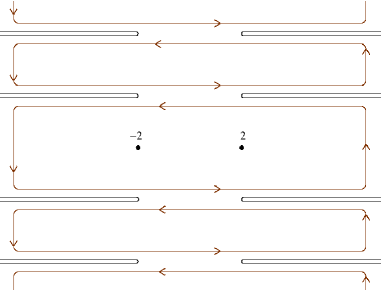
Figure 6: The deformed contour $\Gamma_{\sf O}$.

Restricting the analysis to the solutions that behave asymptotically as $\ln(Y^{(\alpha)}_{(y|-)}/Y^{(\alpha)}_{(y|+)})\rightarrow O(1)$ uniformly as $|u|\rightarrow\infty$ the sum of the vertical segment contributions vanishes as the horizontal size of the rectangles tends to infinity. Then, equation (25) is recovered after inserting relation (27) and observing that several cancelations take place between adjacent integral contributions. In [41] the entire set of TBA equations was retrieved starting from the extended Y-system and adopting certain minimality assumptions for the number of logarithmic singularities in the reference Riemann sheet. These are precisely the analytic conditions fulfilled by the ground state TBA solutions as $\mu_{y}\rightarrow i\pi$. Here, we would like to mention that is possible to show [50] that these assumptions can be relaxed, and that logarithmic singularities of the $\varepsilon_{a}$ and $L_{a}$ functions can lie on the first sheet without affecting the derivation provided they are far enough from the real axis and organized in complexes as required by the Y-system relations. We can summarize the situation at zero chemical potentials in the following proposition.

Proposition 4.1

Let the singularities on the first sheet be organized in complexes such as the following:

$$Y_{Q}(u_{1}^{(-1)})=Y_{Q}(u_{1}^{(-1)}+\frac{2i}{g})=-1;$$

$$Y_{Q+1}((u_{1}^{(-1)}+\frac{i}{g})=Y_{Q-1}((u_{1}^{(-1)}+\frac{i}{g})=1/Y^{(\alpha)}_{(v|Q-1)}(u_{1}^{(-1)}+\frac{i}{g})=0,$$

or

$$Y_{(v|M)}^{(\alpha)}(u_{2}^{(-1)})=Y_{(v|M)}^{(\alpha)}(u_{2}^{(-1)}+\frac{2i}{g})=-1;$$

$$Y_{(v|M+1)}^{(\alpha)}((u_{2}^{(-1)}+\frac{i}{g})=Y_{(v|M-1)}^{(\alpha)}((u_{2}^{(-1)}+\frac{i}{g})=0;\text{ }Y_{M+1}(u_{2}^{(-1)}+\frac{i}{g})=\infty^{2}{\text{ ( double pole )}},$$

or

$$Y_{(w|M)}^{(\alpha)}(u_{3}^{(-1)})=Y_{(w|M)}^{(\alpha)}(u_{3}^{(-1)}+\frac{2i}{g})=-1;$$

$$Y_{(w|M+1)}^{(\alpha)}((u_{3}^{(-1)}+\frac{i}{g})=Y_{(w|M-1)}^{(\alpha)}((u_{3}^{(-1)}+\frac{i}{g})=0,$$

or

$$Y_{(y|-)}^{(\alpha)}(u_{4}^{(-1)})=Y_{(y|-)}^{(\alpha)}(u_{4}^{(-1)}+\frac{2i}{g})=-1;$$

$$Y_{(v|1)}^{(\alpha)}((u_{4}^{(-1)}+\frac{i}{g})=Y_{(w|1)}^{(\alpha)}((u_{4}^{(-1)}+\frac{i}{g})=0;\text{ }Y_{1}(u_{4}^{(-1)}+\frac{i}{g})=\infty^{2}{\text{ ( double pole )}},$$

where, by definition, in equation (4.1): $Y_{(v|0)}^{(\alpha)}=Y_{(y|-)}^{(\alpha)}$, $Y_{0}=0$, and in equations (4.1, 4.1): $Y_{(v|0)}^{(\alpha)}=1/Y_{(w|0)}^{(\alpha)}=Y_{(y|\pm)}^{(\alpha)}$.

Moreover, let the zeroes $u^{(0)}=u^{(-1)}+\frac{i}{g}$ all lie outside the strip $|\text{Im}(u)|<\frac{1}{g}$.
Then the extended Y-system implies the ground state TBA equations.

The ground state equations are modified only when the two points $u^{(-1)}$ and $u^{(-1)}+\frac{2i}{g}$ lie on different sides with respect to the real axis, which can be interpreted as the result of a singularity having crossed the integration contour.

As we shall see in the following sections, the ground state TBA solution at $\mu_{a}=0$ shows indeed several of these complexes of singularities, in the reference sheet but far from the real axis.

5 A useful variant of the TBA equations

To facilitate the numerical implementation of the equations, the following auxiliary functions $E^{(\alpha)}$, $G^{(\alpha)}$, $T^{(\alpha)}$ and $U^{(\alpha)}$ are introduced:

(33) $$\begin{split}E^{(\alpha)}(u)&=\varepsilon^{(\alpha)}_{(y|-)}(u)-\varepsilon^{(\alpha)}_{(y|+)}(u)\\ &=-\sum_{Q}\int_{{\mathbb{R}}}dz\,L_{Q}(z)\left(K(z-i{\textstyle\frac{Q}{g}},u)-K(z+i{\textstyle\frac{Q}{g}},u)\right),\end{split}$$

(34) $$\begin{split}G^{(\alpha)}(u)&=\varepsilon^{(\alpha)}_{(y|-)}(u)+\varepsilon^{(\alpha)}_{(y|+)}(u)\\ &=2\sum_{M}\int_{{\mathbb{R}}}dz\,\left(L^{(\alpha)}_{(v|M)}(z)-L^{(\alpha)}_{(w|M)}(z)\right)\,\phi_{M}(z-u)+2\mu^{(\alpha)}_{y}\\ &-\sum_{Q}\int_{{\mathbb{R}}}dz\,L_{Q}(z)\,\phi_{Q}(z-u),\end{split}$$

(35) $$T^{(\alpha)}(u)=L^{(\alpha)}_{(y|-)}(u)-L^{(\alpha)}_{(y|+)}(u),~{}~{}~{}~{}~{}U^{(\alpha)}(u)=L^{(\alpha)}_{(y|-)}(u)+L^{(\alpha)}_{(y|+)}(u).$$

Using these definitions the TBA equations (5-8) can be recast in the form:

(36) $$\begin{split}\varepsilon^{(\alpha)}_{(w|K)}(u)&=\mu_{(w|K)}^{(\alpha)}+\sum_{M}\int_{{\mathbb{R}}}dz\,L^{(\alpha)}_{(w|M)}(z)\,\phi_{MK}(z-u)+\int_{-2}^{2}dz\,T^{(\alpha)}(z)\,\phi_{K}(z-u),\\ \end{split}$$

(37) $$\begin{split}\varepsilon^{(\alpha)}_{(v|K)}(u)&=\mu_{(v|K)}^{(\alpha)}+\sum_{M}\int_{{\mathbb{R}}}dz\,L^{(\alpha)}_{(v|M)}(z)\,\phi_{MK}(z-u)+\int_{-2}^{2}dz\,(T^{(\alpha)}(z)+E^{(\alpha)}(z))\,\phi_{K}(z-u)\\ &-\sum_{Q}\int_{{\mathbb{R}}}dz\,L_{Q}(z)\,\psi_{QK}(z-u),\end{split}$$

(38) $$\begin{split}\varepsilon_{Q}(u)&=\mu_{Q}+L\,\tilde{E}_{Q}(u)+\sum_{Q^{\prime}}\int_{{\mathbb{R}}}dz\,L_{Q^{\prime}}(z)\,\phi_{Q^{\prime}Q}(z-u)\\ &+\sum_{\alpha}\int_{-2}^{2}dz\,(\varphi^{(\alpha)}(z)+\frac{1}{2}U^{(\alpha)}(z))\left(K(z,u-i{\textstyle\frac{Q}{g}})-K(z,u+i{\textstyle\frac{Q}{g}})\right)\\ &-\frac{1}{2}\sum_{\alpha}\int_{-2}^{2}dz\,T^{(\alpha)}(z)\,\phi_{Q}(z-u)+\sum_{\alpha,M}\int_{{\mathbb{R}}}dz\,L^{(\alpha)}_{(v|M)}(z)\,\psi_{MQ}(z-u)\\ &-\sum_{\alpha}\left(\int_{-\infty}^{-2}dz+\int_{2}^{\infty}dz\right)\,E^{(\alpha)}(z)\,\chi_{Q}(z,u),\end{split}$$

with

(39) $$\chi_{Q}(z,u) =\left(\int_{-\infty}^{-2}dt+\int_{2}^{\infty}dt\right)\,K_{\Gamma}^{[2]}(z-t)\left(K(t,u-i{\textstyle\frac{Q}{g}})-K(t,u+i{\textstyle\frac{Q}{g}})\right),$$

where the last term of (38) is obtained from the last term of (10) using the following important relation discussed in Appendix D of [41]:

(40) $$\begin{split}\sum_{Q^{\prime}}L_{Q^{\prime}}\ast K_{Q^{\prime}Q}^{\Sigma}(v)&=\sum_{Q^{\prime}}L_{Q^{\prime}}\ast\oint_{\bar{\gamma}_{\sf x}}ds\;\phi_{Q^{\prime},y}^{(\alpha)}(s)\oint_{\bar{\gamma}_{\sf x}}dt\;K_{\Gamma}^{\left[2\right]}(s-t)\phi_{y,Q}(t,v)\\ &=-\oint_{\bar{\gamma}_{\sf x}}ds\;\ln Y_{y}^{(\alpha)}(s)\oint_{\bar{\gamma}_{\sf x}}K_{\Gamma}^{\left[2\right]}(s-t)\phi_{y,Q}(t,v).\end{split}$$

To further optimize the implementation of the equations, we have minimized the number of terms that depend on the two variables $z$ and $u$ separately . The last term appearing on the rhs of (37) was rewritten considering relation (E8) in [41]:

(41) $$\begin{split}-\sum_{Q}\int_{{\mathbb{R}}}dz\,L_{Q}(z)\,\phi_{Q,(v|K)}(z,u)&=\int_{-2}^{2}dz\,E^{(\alpha)}(z)\,\phi_{K}(z-u)\\ &-\sum_{Q}\int_{{\mathbb{R}}}dz\,L_{Q}(z)\psi_{QK}(z-u),\end{split}$$

with

(42) $$\psi_{QM}(u)=\sum_{j=0}^{M-1}\phi_{Q-M+2j}(u)=\left\{\begin{array}[]{rl}&{\stackrel{{\scriptstyle\mbox{\tiny{step 2}}}}{{\sum}}}_{j=|Q-M|}^{|Q+M|-2}\;\phi_{j}(u)\;;\;Q>M;\\ \\ &{\stackrel{{\scriptstyle\mbox{\tiny{step 2}}}}{{\sum}}}_{j=|Q-M|+2}^{|Q+M|-2}\;\phi_{j}(u)\;;\;Q\leq M.\end{array}\right.$$

Similarly for the penultimate term on the rhs of (38) we have used

(43) $$\begin{split}\sum_{\alpha,M}\int_{{\mathbb{R}}}dz\,L^{(\alpha)}_{(v|M)}(z)\,\phi_{(v|M),Q}(z,u)&=\sum_{\alpha}\int_{-2}^{2}dz\,\varphi^{(\alpha)}(z)\,\left(K(z,u-i{\textstyle\frac{Q}{g}})-K(z,u+i{\textstyle\frac{Q}{g}})\right)\\ &-\sum_{\alpha,M}\int_{{\mathbb{R}}}dz\,L^{(\alpha)}_{(v|M)}(z)\psi_{MQ}(z-u),\end{split}$$

with

(44) $$\varphi^{(\alpha)}(u) =\sum_{N}\int_{{\mathbb{R}}}dz\,L^{(\alpha)}_{(v|N)}(z)\,\phi_{N}(z-u).$$

The equations for the pseudoenergies used in the numerical work to be described shortly correspond to an appropriately discretized version of (36-44) where the infinite sums are truncated to a finite number of terms $N_{max}$ and the integrals performed only in the range $(-z_{max};z_{max})$. The chemical potentials are set to zero but for those associated to the fermionic particles $(y|\pm)$ where $\mu_{y}=\mu^{(1)}_{y}=-\mu^{(2)}_{y}$. The results obtained and partially discussed in this paper correspond to the parameters in the ranges reported in Table 2.

Convergence threshold for $L_{a}$	$\epsilon=1\times 10^{-14}$
Coupling	$g\in(0,1]$
Scale	$L\in(0,10]$
Integration range ($-z_{max};z_{max}$)	$z_{max}=50$
Number of $\Delta z$ intervals in ($-2;2$)	$N_{F}\in(1,150]$
Truncation	$N_{max}\in[2,15]$
Chemical potentials for $(y|\pm)$	$\mu_{y}\in\{(-10,10)\times[0,\pi)\}$

Table 2: Parameter ranges.

6 TBA numerical solution: the real axis

The functions $L_{a}(u)$, solutions of the thermodynamic Bethe Ansatz equations, are represented in Figure 7 to Figure 12.

Figure 7: Solutions $\text{Re}(L_{Q})$: $L=4$, $g=0.5$, $\mu_{y}=0$.

Figure 7 shows the real parts of $L_{Q}(u)$ for $Q=1$ and $Q=2$ at $L=4$, $g=0.5$ and $\mu_{y}=0$. The solutions are well localized around the origin, tend exponentially to the asymptotic value $L_{Q}^{0}=0$ and in addition $L_{1}(u)\gg L_{2}(u)$. These are general features of the solutions of this TBA: at moderate values of the coupling constant $g$ the difference between $L_{a}(u)$ and its asymptotic value $L_{a}^{0}$ is always well localized about the origin and a given component $L_{a}(u)$ strongly dominates over the next, ie $L_{a}(u)\gg L_{a+1}(u)$. This justifies both the relatively small range of integration and the truncation of the sums to a finite number of terms $N_{max}$. Unfortunately, both the localization and the subdominancy features get -for generic values of $\mu_{y}$ and $L$- worse and worse as $g$ is increased above $1$ and in the strong coupling regime one has to push the computer internal resources to the extreme. Figure 8 shows the results for the excitations of type $v$ and $w$ with $M=1$, they also reach the asymptotic values $L^{0}_{(v|1)}=L^{0}_{(w|1)}=\ln{\textstyle\frac{4}{3}}$ exponentially fast in the large $|u|$ region. Figure 9 shows instead the real parts of $L(u)$ for the excitations $v,w$ with $M=2$, they are smaller and reach the asymptotic value $L^{0}_{(v|2)}=L^{0}_{(w|2)}=\ln{\textstyle\frac{9}{8}}$ faster that the $M=1$ cases. Again we see that the $M$ components dominate over the $M+1$ ones.

Figure 8: Solutions $\text{Re}(L_{(v|1)})$, $\text{Re}(L_{(w|1)})$: $L=4$, $g=0.5$, $\mu_{y}=0$.

Figure 9: Solutions $\text{Re}(L_{(v|2)})$, $\text{Re}(L_{(w|2)})$: $L=4$, $g=0.5$, $\mu_{y}=0$.

The imaginary parts of $L(u)$ for the excitations $Q$, $v$ and $w$ vanish within our computer working precision.

Figure 10: Solutions $\text{Re}(L_{(y|\pm)})$: $L=4$, $g=0.5$, $\mu_{y}=0$.

Figure 10 compares the real parts for the $(y|\pm)$ fermionic particles. These solutions have a physical interpretation in terms of particle and hole densities only in the rapidity range $u\in(-2,2)$ [36, 37, 38].

Indeed, one can see cusps at $u=\pm 2$ highlighted in Figure 11. Outside the physical interval $(-2,2)$ both functions tend to the corresponding asymptotic value $\ln 2$.

The imaginary parts are depicted in Figure 12 and they vanish for $u\in(-2,2)$, confirming that only in such interval the pseudoenergies $\varepsilon^{(\alpha)}_{(y|\pm)}(u)$ are physically meaningful.

Figure 11: The square root branch point of $\text{Re}(L_{y})$: $L=4$, $g=0.5$, $\mu_{y}=0$.

Figure 12: Solutions $\text{Im}(L_{(y|\pm)})$: $L=4$, $g=0.5$, $\mu_{y}=0$.

The solutions of the TBA equations expressed in terms of the functions $L_{a}(u)$ have, in principle, a maximum precision of the order of the threshold of convergence shown in Table 2. In fact, the solutions are mainly affected by errors due to the discretisation of the domain of integration and the truncation of the infinite sums. The TBA equations are non-linear, this makes it difficult to assess a priori the magnitude of those errors but we have estimated the precision by comparing solutions at various values of $N_{max}$, $z_{max}$ and $\Delta z$. As a result of this analysis, in the range of parameters reported in Table 2, the estimated precision is between $10^{-6}$ and $10^{-9}$.

7 $E=0$ protected state and scale quantisation

The ground state energy of the model is obtained from the pseudoenergies for the $Q$-particles as:

(45) $$E_{0}(L)=-\sum_{Q=1}^{\infty}\int_{{\mathbb{R}}}\frac{du}{2\pi}\frac{d\tilde{p}^{Q}}{du}\,L_{Q}(u),$$

where

(46) $$\tilde{p}^{Q}(u)=gx(u-iQ/g)-gx(u+iQ/g)+iQ,$$

is the mirror theory momentum. In ${\cal N}=4$ SYM the true vacuum state is protected by supersymmetry and from the TBA this state is found by sending the chemical potential for the fermionic particles to [52]

(47) $$\mu_{y}=\mu_{y}^{(1)}=-\mu_{y}^{(2)}\rightarrow i\pi\quad\Longrightarrow\quad E_{0}(L,\mu_{y},g)\rightarrow 0\quad\forall g,L,$$

while all the other chemical potentials are kept at zero.

Figure 13 shows the occurrence of this condition at different values of the parameters while Figure 14 compares the numerical result with the asymptotic estimate given in [51]:

(48) $$E_{0}\sim-\sum_{Q=1}^{\infty}\int_{{\mathbb{R}}}\frac{du}{2\pi}\frac{d\tilde{p}^{Q}}{du}\,\ln\left(1+16Q^{2}\sin^{2}\!\frac{h}{2}e^{-L\tilde{E}_{Q}(u)}\right)\;;\;\mbox{ general $h$, large $L$.}$$

with $h=-i\mu_{y}-\pi$.

Figure 13: $E_{0}$ versus $\mu_{y}$ and $g$: $L=4$.

Figure 14: $E_{0}$, numerical versus the exact asymptotic result: $L=4$, $g=0.5$.

Further, from the point of view of ${\cal N}=4$ super Yang-Mills the parameter $L$ should be restricted to strictly positive integer values. In fact, $L$ is related to the number of elementary operators building the composite trace operator of which we would like to determine the anomalous dimension. On the contrary, within the TBA setup $L$ is simply the inverse of the temperature and does not necessarily need be quantised. In [51] and more generally in [41] a drastic simplification of the analytic properties of the solutions was observed at integer $L$ but, up to now, these mathematical facts have not been neatly linked to the gauge theory origin of the equations.

Indeed, the pseudoenergies change smoothly on the real axis with the scale and the chemical potential $\mu_{y}$ giving a smooth variation of $E_{0}(L,\mu_{y})$, as shown in Figures 15 and 16.
Figure 15 corresponds to a truncation at $N_{max}=2$, and we see that the energy tends uniformly to zero as $\mu_{y}\rightarrow i\pi$. Notice also that, regardless of $\mu_{y}$, there is a particular value of $L\approx 2.3$ where the curves simultaneously intersect the horizontal axis.

Figure 15: $E_{0}$ versus $L$, $\mu_{y}$: $g=0.5$, $N_{max}=2$.

Figure 16 corresponds to a truncation $N_{max}=5$, again the ground state energy tends uniformly to zero as $\mu_{y}\rightarrow i\pi$ and at $L\approx 2.07$ the various curves intersect on the horizontal axis. Increasing $N_{max}$ we observed that the intersection point approaches $L=2$, but unfortunately the program fails to converge at $L=2$ for $N_{max}\geq 8$.

Figure 16: $E_{0}$ versus $L$, $\mu_{y}$: $g=0.5$, $N_{max}=5$.

8 Mapping the complex plane

In this section we shall describe qualitatively the analytic properties of the TBA solutions in the complex rapidity plane. Following [24, 25] the solutions for complex values of the rapidity were first obtained in the fundamental strip $|\text{Im}(u)|\leq{\textstyle\frac{1}{g}}$ starting from the $L_{a}(u)$ computed on the real axis and using the TBA equations as integral representations for the pseudoenergies.

Then, the solutions were calculated in the other strips, defined as

(49) $$\begin{split}{\text{Strip}}^{(+k)}&=\{u\;/\;\text{Re}(u)\in(-\infty,+\infty)\;,\;\text{Im}(u)\in(+{\textstyle\frac{k}{g}},+{\textstyle\frac{k+1}{g}})\},\\ {\text{Strip}}^{(-k)}&=\{u\;/\;\text{Re}(u)\in(-\infty,+\infty)\;,\;\text{Im}(u)\in(-{\textstyle\frac{k+1}{g}},-{\textstyle\frac{k}{g}})\},\end{split}$$

with $k=1,2,\cdots$, using the basic Y-system (14-17) and connecting two points in a given strip $k$ to a point outside it, as exemplified in Figure 17. In this way the whole complex plane can be mapped.

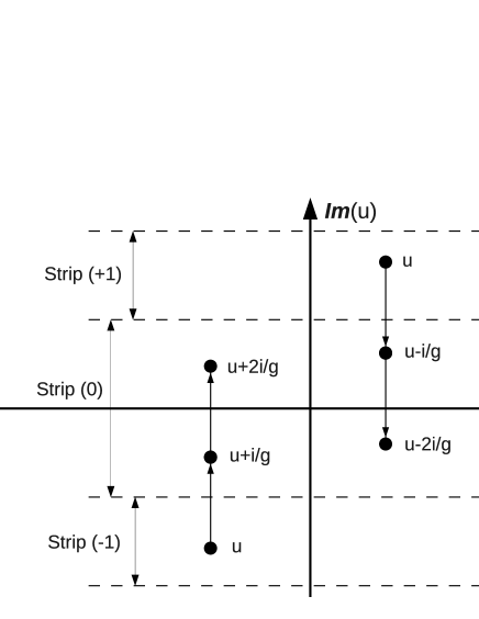
Figure 17: Mapping of the complex plane of rapidity $u$.

Notice that the basic Y-system does not contain a functional equation for $Y^{(\alpha)}_{(y|+)}$, to overcome this problem we used equation (34)

(50) $$\varepsilon^{(\alpha)}_{(y|+)}(u)=G^{(\alpha)}(u)-\varepsilon^{(\alpha)}_{(y|-)}(u),$$

with

(51) $$\begin{split}G^{(\alpha)}(u)&=\sum_{M}{\cal L}^{(\alpha)}_{M}*\phi_{M}(u)+2\mu^{(\alpha)}_{y},\end{split}$$

and ${\cal L}^{(\alpha)}_{M}(u)=2L^{(\alpha)}_{(v|M)}(u)-2L^{(\alpha)}_{(w|M)}(u)-L_{M}(u)$ and analytically continued it to a generic strip in the complex plane:

(52) $$u\in{\text{Strip}}^{(\pm k)}\;;\;G^{(\alpha)}(u)=\sum_{M}{\cal L}^{(\alpha)}_{M}*\phi_{M}(u)+2\mu^{(\alpha)}_{y}+\sum_{n=1}^{k}{\cal L}^{(\alpha)}_{n}(u\mp{\textstyle\frac{i}{g}}n).$$

The last term on the rhs of (52) comes from the residues of the simple pole singularities in $\phi_{M}(u)$. In order to unveil the analytical properties of the Y functions in the complex rapidity plane we have introduced the functions [25]

(53) $$F^{\pm}_{a}(u)=\frac{|1+Y^{\pm 1}_{a}(u)|}{1+|1+Y^{\pm 1}_{a}(u)|}\in[0,1],$$

and considered the special or critical points $u^{(0)}$,$u^{(-1)}$,$u^{(\infty)}$ such that

(54) $$Y_{A}(u^{(0)})=0\;\;;\;\;Y_{A}(u^{(-1)})=-1\;\;;\;\;Y_{A}(u^{(\infty)})\rightarrow\infty.$$

Table 3 summarizes the values assumed by $F^{(\pm)}_{a}(u)$ in correspondence to these points. The functions $F^{+}_{a}$ emphasize better the $u^{(-1)}$ and $u^{(\infty)}$ points, on the contrary the function $F^{-}_{a}$ are best suited to highlight the points $u^{(0)}$ and $u^{(-1)}$.

$u$	$u^{(0)}$	$u^{(-1)}$	$u^{(\infty)}$
$Y_{a}(u)$	0	-1	$\infty$
$F^{+}_{a}(u)$	${\textstyle\frac{1}{2}}$	0	1
$F^{-}_{a}(u)$	1	0	${\textstyle\frac{1}{2}}$

Table 3: $F^{\pm}$ values corresponding to $u^{(0)}$, $u^{(-1)}$, $u^{(\infty)}$.

Figure 18 shows a three dimensional plot of $F^{-}_{1}(u)$ where the square root branch cuts emerge and we also see peaks at zero ($u^{(-1)}$) and peaks at one ($u^{(0)}$). A picture of this kind is certainly nice looking but it is not very easy to interpret.

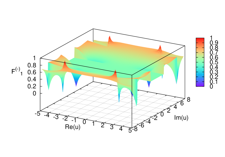
Figure 18: 3D plot of $F^{-}_{1}(u)$: $L=4$, $g=0.5$, $\mu_{y}=0$.

We therefore consider two dimensional plots with contour lines, in which the value of the functions $F^{(\pm)}_{a}$ is encoded using a scale of colours. Blue corresponds to $F^{(\pm)}_{a}=0$ while red to $F^{(\pm)}_{a}=1$. Figure 19 plots $F^{-}_{1}$, where the critical points of type $u^{(0)}$ and $u^{(-1)}$ and the branch cuts are easily recognisable.

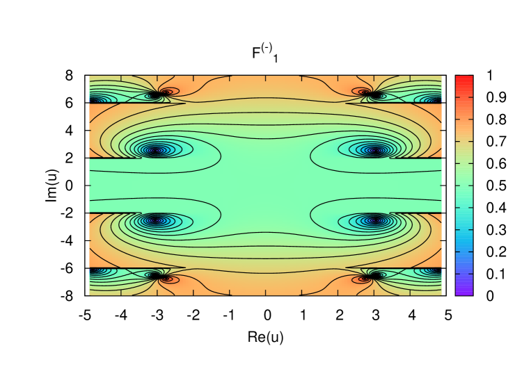
Figure 19: Contour plot of $F^{-}_{1}(u)$: $L=4$, $g=0.5$, $\mu_{y}=0$.

The basic Y-system relates poles and zeroes between adjacent strips on the reference sheet, so that complexes or strings of critical points emerge. As an example of these phenomena, we shall highlight the link between points $u^{(0)}$, $u^{(-1)}$ and $u^{(\infty)}$ induced by equation (14) at $Q=1$:

(55) $$Y_{1}(u-{\textstyle\frac{i}{g}})Y_{1}(u+{\textstyle\frac{i}{g}})=\left(1+Y_{2}(u)\right){\left(\frac{Y_{(y|-)}^{(1)}(u)}{1+Y_{(y|-)}^{(1)}(u)}\right)}^{2},$$

where we have used the symmetry $Y_{(y|-)}^{(1)}=Y_{(y|-)}^{(2)}$ for $\mu^{(\alpha)}_{y}=0$. Equation (55) shows that there are relations between the zeroes and the poles of the functions

(56) $$Y_{1},\,Y_{2},\,(1+Y_{2}),\,Y^{(1)}_{(y|-)},\,(1+Y^{(1)}_{(y|-)}).$$

From Figure 20 we see that the functions $F^{\pm}_{(y|-)}(u)$ vanish at $u=u^{(-1)}\approx(3.7,4.4)\in\text{Strip}^{(+2)}$ (in blue). At this point the rhs of equation (55) tends to infinity, this implies that $F^{+}_{1}(u)=1$ at $u=u^{(\infty)}\approx(3.7,6.4)\in\text{Strip}^{(+3)}$ (a double pole of $Y_{1}$) which can be clearly spotted in Figure 21 (in red). Consider now Figure 21, the functions $F^{\pm}_{1}(u)$ show the existence of zeroes at $u=u^{(-1)}\approx(3.1,6.5)\in\text{Strip}^{(+3)}$ (in blue) so at that point the lhs of (55) is equal to one. In turn, this implies that $F^{-}_{2}(u)=1$ at $u=u^{(0)}\approx(3.1,4.5)\in\text{Strip}^{(+2)}$, this also clearly emerges from Figure 22 (in red).

This is not sufficient to guarantee compatibility between the lhs and rhs of (55), in fact also the part related to $Y^{(1)}_{(y|-)}$ on the rhs must tend to one. This implies that $F^{+}_{(y|-)}(u)$ must have a critical point at $u=u^{(\infty)}\approx(3.1,4.5)\in\text{Strip}^{(+2)}$ which presence is clearly observable in Figure 20 (in red).

Finally, the reader can see that the function $F^{+}_{2}(u)$ plotted in Figure 22 vanishes at $u=u^{(-1)}\approx(2.8,4.7)\in\text{Strip}^{(+2)}$ (in blue), this is related to a critical point $u^{(0)}\approx(2.8,6.7)\in\text{Strip}^{(+3)}$(in red) observable in $F^{-}_{1}(u)$ plotted in Figure 21. Notice that the picture emerging from this quick inspection matches perfectly the complexes of critical points defined in Proposition 4.1. The interest for the classification of these complexes or strings is not purely academic but it is actually an important preliminary step for the classification of the excited states of the theory.

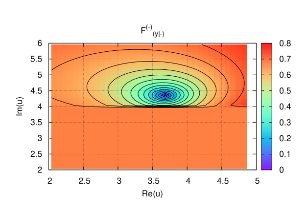
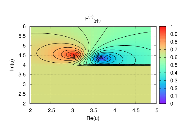
Figure 20: Details of $F^{\pm}_{(y|-)}(u)$: $L=4$, $g=0.5$, $\mu_{y}=0$.

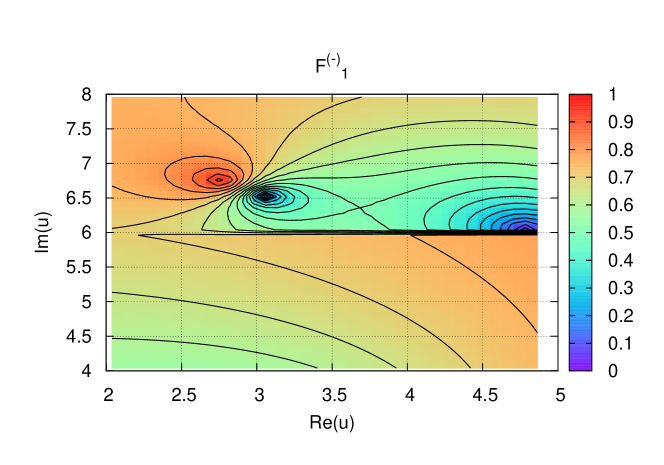
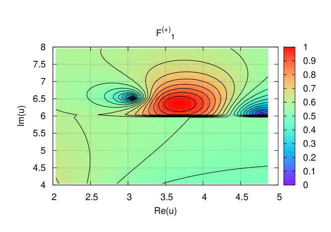
Figure 21: Details of $F^{\pm}_{1}(u)$ : $L=4$, $g=0.5$, $\mu_{y}=0$.

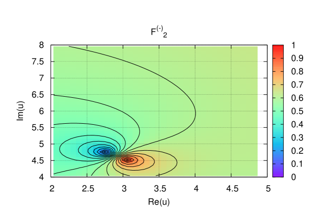
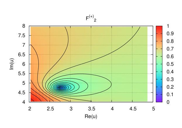
Figure 22: Details of $F^{\pm}_{2}(u)$: $L=4$, $g=0.5$, $\mu_{y}=0$.

9 Conclusions

The correspondence between strings and gauge theories provides exactly soluble models with remarkable properties. These important systems can be studied using the powerful tools developed over the years in the integrability context for the study of models mainly relevant to condensed matter physics in low dimensions.

A main objective of this article is to describe preliminary numerical results concerning a new variant of the TBA equations for the $\text{AdS}_{5}/\text{CFT}_{4}$ correspondence in the attempt to reveal the analytic properties of their solutions.

Studying the evolution of the ground state energy at different values of the scale and the chemical potential, we have checked that -as predicted by supersymmetry- the equations correctly lead to a vacuum state with zero energy as $\mu_{y}\rightarrow i\pi$ at arbitrary scale $L$.

It was then possible to explore the functions $F^{(\pm)}_{a}$ in the complex plane of the rapidity, allowing us to study the zeroes and the singularities of the functions $Y_{a}(u)$ and $1+Y_{a}(u)$. We have seen that the basic Y-system relates points between adjacent strips of the complex plane and verified the presence of square root branch cuts exactly at the points predicted by [41] and summarized in Table 1. These results confirm that the analytic properties of the $\text{AdS}_{5}/\text{CFT}_{4}$ thermodynamic Bethe Ansatz equations are very different from those of the relativistic integrable quantum field theories. The Y functions live on a complicated and -up to now- only superficially explored Riemann surface with an infinite number of square root branch points.

Finally our set of programs should be easily adaptable to other non-linear integral equations, as for example those for the $\text{AdS}_{4}/\text{CFT}_{3}$ correspondence, linking the type IIA string theory on $\text{AdS}_{4}\times{\mathbb{C}}{\mathbb{P}}^{3}$ to the Chern-Simons model with supersymmetry ${\cal N}=6$ in three dimensions [53, 54, 55].

10 Acknowledgements

RT thanks the organizers of the conference “Infinite Analysis 10: Developments in Quantum Integrable Systems” and especially Atsuo Kuniba, Tomoki Nakanishi and Masato Okado for the invitation to speak and the kind hospitality.

We acknowledge the INFN grants IS PI14, FI11, PI11 and the University PRIN 2007JHLPEZ for travel financial support.

Appendix A The S-matrix elements

Here we report the scalar factors $S_{AB}$ involved in the definition of kernels in the TBA equations (5-8).

(57) $$S_{y,Q}(u,z)=S_{Q,y}(z,u)=\left(\frac{x(z-\frac{i}{g}Q)-x(u)}{x(z+\frac{i}{g}Q)-x(u)}\right)\sqrt{\frac{x(z+\frac{i}{g}Q)}{x(z-\frac{i}{g}Q)}}.$$

(58) $$\begin{split}S_{(v|M),Q}(u,z)=&S_{Q,(v|M)}(z,u)=\left(\frac{x(z-\frac{i}{g}Q)-x(u+\frac{i}{g}M)}{x(z+\frac{i}{g}Q)-x(u+\frac{i}{g}M)}\right)\left(\frac{x(z+\frac{i}{g}Q)}{x(z-\frac{i}{g}Q)}\right)\\ &\times\left(\frac{x(z-\frac{i}{g}Q)-x(u-\frac{i}{g}M)}{x(z+\frac{i}{g}Q)-x(u-\frac{i}{g}M)}\right)\prod_{j=1}^{M-1}\left(\frac{z-u-\frac{i}{g}(Q-M+2j)}{z-u+\frac{i}{g}(Q-M+2j)}\right),\end{split}$$

(59) $$S_{M}(u)=\left(\frac{u-\frac{i}{g}M}{u+\frac{i}{g}M}\right),$$

(60) $$S_{KM}(u) =\prod_{k=1}^{K}\prod_{l=1}^{M}S_{((K+2-2k)-(M-2l))}(u)$$

$$=\left(\frac{u-{\textstyle\frac{i}{g}}|K-M|}{u+\frac{i}{g}|K-M|}\right)\left(\frac{u-\frac{i}{g}(K+M)}{u+\frac{i}{g}(K+M)}\right)\prod_{k=1}^{\text{min}(K,M)-1}\left(\frac{u-\frac{i}{g}(|K-M|+2k)}{u+\frac{i}{g}(|K-M|+2k)}\right)^{2}.$$

The elements $S^{\Sigma}_{Q^{\prime}Q}$ are:

(61) $$S^{\Sigma}_{Q^{\prime}Q}(z,u)=(S_{Q^{\prime}Q}(z-u))^{-1}(\Sigma_{Q^{\prime}Q}(z,u))^{-2},$$

where $\Sigma_{Q^{\prime}Q}$ is the improved dressing factor for the mirror bound states

(62) $$\Sigma_{Q^{\prime}Q}(z,u)=\prod_{k=1}^{Q^{\prime}}\prod_{l=1}^{Q}\left(\frac{1-\frac{1}{x(z+\frac{i}{g}(Q^{\prime}+2-2k))x(u+\frac{i}{g}(Q-2l))}}{1-\frac{1}{x(z+\frac{i}{g}(Q^{\prime}-2k))x(u+\frac{i}{g}(Q+2-2l))}}\right)\sigma_{Q^{\prime}Q}(z,u),$$

with $\sigma_{Q^{\prime}Q}$ evaluated in the mirror kinematics. A precise analytic expression for the mirror improved dressing factor has been given in [43], and a more compact integral representation in [37]. The equivalence between these two results was proved in [41] .

References

- [1] J.M. Maldacena, The large limit of superconformal field theories and supergravity, Adv. Theor. Math. Phys.2 (1998) 231 [arXiv:hep-th/9711200].
-
[2]
S.S. Gubser, I.R. Klebanov and A.M. Polyakov,
Gauge theory correlators from non-critical string theory,
Phys. Lett. B428 (1998) 105
[arXiv:hep-th/9802109];
E. Witten, Anti-de Sitter space and holography, Adv. Theor. Math. Phys.2 (1998) 253, [arXiv:hep-th/9802150]. - [3] I. Bena, J. Polchinski and R. Roiban, Hidden symmetries of the superstring, Phys. Rev. D69 (2004) 046002 [arXiv:hep-th/0305116].
-
[4]
V.A. Kazakov, A. Marshakov, J.A. Minahan and K. Zarembo,
Classical/quantum integrability in AdS/CFT,
JHEP05 (2004) 024
[arXiv:hep-th/0402207];
V.A. Kazakov, K. Zarembo, Classical/quantum integrability in non-compact sector of AdS/CFT, JHEP10 (2004) 060 [arXiv:hep-th/0410105]. - [5] J.A. Minahan and K. Zarembo, The Bethe Ansatz for Super Yang-Mills, JHEP03 (2003) 013 [arXiv:hep-th/0212208].
- [6] G. ’t Hooft, A planar diagram theory for strong interactions, Nucl. Phys. B72 (1974) 461.
- [7] H. Bethe, On the theory of metals. 1. Eigenvalues and eigenfunctions for the linear atomic chain, Z. Phys.71 (1931) 205;
-
[8]
N. Beisert and M. Staudacher,
The SYM integrable super spin chain,
Nucl. Phys. B670 (2003) 439
[arXiv:hep-th/0307042];
M. Staudacher, The factorized S-matrix of CFT/AdS, JHEP05 (2005) 054 [arXiv:hep-th/0412188];
N. Beisert and M. Staudacher, Long-range Bethe Ansatz for gauge theory and strings, Nucl. Phys. B727 (2005) 1 [arXiv:hep-th/0504190];
G. Arutyunov, S. Frolov and M. Staudacher, Bethe Ansatz for quantum strings, JHEP10 (2004) 016 [arXiv:hep-th/0406256];
R. Janik, The superstring worldsheet S-matrix and crossing symmetry, Phys. Rev. D73 (2006) 086006 [arXiv:hep-th/0603038];
N. Beisert, R. Hernandez and E. Lopez, A crossing symmetric phase for strings, JHEP11 (2006) 070 [arXiv:hep-th/0609044]. - [9] N. Beisert, B. Eden and M. Staudacher, Transcendentality and crossing, J. Stat. Mech.0701 (2007) P021 [arXiv:hep-th/0610251].
-
[10]
C. Sieg and A. Torrielli,
Wrapping interactions and the genus expansion of the 2-point function of composite operators,
Nucl. Phys. B723, (2005) 3
[arXiv:hep-th/0505071];
T. Fischbacher, T. Klose and J. Plefka, Planar plane-wave matrix theory at the four loop order: Integrability without BMN scaling, JHEP0502 (2005) 039 [arXiv:hep-th/0412331]. - [11] J. Ambjorn, R.A. Janik and C. Kristjansen, Wrapping interactions and a new source of corrections to the spin-chain string duality, Nucl. Phys. B736 (2006) 288 [arXiv:hep-th/0510171];
-
[12]
C.N. Yang and C.P. Yang,
One-dimensional chain of anisotropic spin-spin interactions. I: Proof of Bethe’s hypothesis for ground state in a finite system,
Phys. Rev.150 (1966) 321;
C.N. Yang, Some exact results for the many body problems in one dimension with repulsive delta function interaction, Phys. Rev. Lett.19 (1967) 1312;
R.J. Baxter, Partition function of the eight-vertex model, Ann. Phys.70 (1972) 193;
L.D. Faddeev, E.K. Sklyanin and L.A. Takhtajan, The quantum inverse problem method. 1, Theor. Math. Phys.40 (1980) 688 [Teor. Mat. Fiz.40 (1979) 194]; A.B. Zamolodchikov and A.B. Zamolodchikov, Factorized S-matrices in two dimensions as the exact solutions of certain relativistic quantum field models, Annals Phys.120 (1979) 253. -
[13]
N. Beisert,
The su(2—2) dynamic S-matrix,
Adv. Theor. Math. Phys.12 (2008) 945
[arXiv:hep-th/0511082];
M.J. Martins and C.S. Melo, The Bethe Ansatz approach for factorizable centrally extended S-matrices, Nucl. Phys. B785 (2007) 246 [arXiv:hep-th/0703086]. - [14] Z. Bajnok and R. A. Janik, Four-loop perturbative Konishi from strings and finite size effects for multiparticle states, Nucl. Phys. B807, 625 (2009) [arXiv:0807.0399 [hep-th]].
-
[15]
M. Lüscher,
Volume dependence of the energy spectrum in massive quantum field theories.
1. Stable particle states,
Commun. Math. Phys.104 (1986) 177;
M. Lüscher, On a relation between finite size effects and elastic scattering processes, Lecture given at Cargese Summer Inst., Cargese, France, Sep 1-15, 1983. - [16] T.R. Klassen and E. Melzer, On the relation between scattering amplitudes and finite size mass corrections in QFT, Nucl. Phys. B362 (1991) 329.
-
[17]
F. Fiamberti, A. Santambrogio, C. Sieg and D. Zanon,
Wrapping at four loops in N=4 SYM,
Phys. Lett. B666 (2008) 100
[arXiv:0712.3522 [hep-th]];
F. Fiamberti, A. Santambrogio, C. Sieg and D. Zanon, Anomalous dimension with wrapping at four loops in N=4 SYM, Nucl. Phys. B805 (2008) 231 [arXiv:0806.2095 [hep-th]]. - [18] M. Beccaria, V. Forini, T. Lukowski and S. Zieme, Twist-three at five loops, Bethe Ansatz and wrapping, JHEP0903, (2009) 129 [arXiv:0901.4864 [hep-th]].
- [19] Z. Bajnok, A. Hegedus, R. A. Janik and T. Lukowski, Five loop Konishi from AdS/CFT, Nucl. Phys. B827 (2010) 426 [arXiv:0906.4062 [hep-th]].
- [20] Al.B. Zamolodchikov, Thermodynamic Bethe Ansatz in relativistic models. Scaling three state Potts and Lee-Yang models, Nucl. Phys. B342, 695 (1990).
- [21] C. N. Yang and C. P. Yang, Thermodynamics of a one-dimensional system of bosons with repulsive delta-function interaction, J. Math. Phys.10, 1115 (1969).
- [22] T.R. Klassen and E. Melzer, The thermodynamics of purely elastic scattering theories and conformal perturbation theory, Nucl. Phys. B350 (1991) 635.
- [23] V.V. Bazhanov, S.L. Lukyanov and A.B. Zamolodchikov, Quantum field theories in finite volume: Excited state energies, Nucl. Phys. B489, 487 (1997) [arXiv:hep-th/9607099].
- [24] P. Dorey and R. Tateo, Excited states by analytic continuation of TBA equations, Nucl. Phys. B482 (1996) 639 [arXiv:hep-th/9607167].
- [25] P. Dorey and R. Tateo, Excited states in some simple perturbed conformal field theories, Nucl. Phys. B515 (1998) 575 [arXiv:hep-th/9706140].
- [26] P. Dorey, A. Pocklington, R. Tateo and G. Watts, TBA and TCSA with boundaries and excited states, Nucl. Phys. B525, (1998) 641 [arXiv:hep-th/9712197].
- [27] C. Destri and H. J. de Vega, New thermodynamic Bethe Ansatz equations without strings, Phys. Rev. Lett.69 (1992) 2313.
- [28] D. Fioravanti, A. Mariottini, E. Quattrini and F. Ravanini, Excited state Destri-De Vega equation for sine-Gordon and restricted sine-Gordon models, Phys. Lett. B390 (1997) 243 [arXiv:hep-th/9608091].
- [29] G. Feverati, F. Ravanini and G. Takacs, Truncated conformal space at c = 1, nonlinear integral equation and quantization rules for multi-soliton states, Phys. Lett. B430, 264 (1998) [arXiv:hep-th/9803104].
- [30] D. Fioravanti and M. Rossi, On the commuting charges for the highest dimension SU(2) operator in planar SYM, JHEP0708 (2007) 089 [arXiv:0706.3936 [hep-th]].
- [31] L. Freyhult, A. Rej and M. Staudacher, A generalized scaling function for AdS/CFT, J. Stat. Mech.0807 (2008) P07015 [arXiv:0712.2743 [hep-th]].
- [32] D. Bombardelli, D. Fioravanti and M. Rossi, Large spin corrections in SYM sl(2): still a linear integral equation, Nucl. Phys. B810 (2009) 460 [arXiv:0802.0027 [hep-th]].
- [33] G. Feverati, D. Fioravanti, P. Grinza and M. Rossi, Hubbard’s adventures in N = 4 SYM-land? Some non-perturbative considerations on finite length operators, J. Stat. Mech.0702 (2007) P001 [arXiv:hep-th/0611186].
- [34] G. Arutyunov and S. Frolov, On string S-matrix, bound states and TBA, JHEP0712 (2007) 024 [arXiv:0710.1568 [hep-th]].
- [35] G. Arutyunov and S. Frolov, String hypothesis for the mirror, JHEP0903, 152 (2009) [arXiv:0901.1417 [hep-th]].
- [36] D. Bombardelli, D. Fioravanti and R. Tateo, Thermodynamic Bethe Ansatz for planar AdS/CFT: a proposal, J. Phys. A42 (2009) 375401 [arXiv:0902.3930 [hep-th]].
-
[37]
N. Gromov, V. Kazakov, A. Kozak and P. Vieira,
Exact spectrum of anomalous dimensions of planar N = 4 Supersymmetric Yang-Mills theory: TBA and excited states,
Lett. Math. Phys.91, 265 (2010)
[arXiv:0902.4458 [hep-th]].
(arXiv Title: Integrability for the full spectrum of planar AdS/CFT II.) - [38] G. Arutyunov and S. Frolov, Thermodynamic Bethe Ansatz for the mirror model, JHEP0905 (2009) 068 [arXiv:0903.0141 [hep-th]].
-
[39]
N. Gromov, V. Kazakov and P. Vieira,
Exact spectrum of anomalous dimensions of planar N=4 Supersymmetric Yang-Mills theory,
Phys. Rev. Lett.103, 131601 (2009)
[arXiv:0901.3753 [hep-th]].
(arXiv Title:Integrability for the full spectrum of planar AdS/CFT.) - [40] G. Arutyunov, S. Frolov and R. Suzuki, Exploring the mirror TBA, JHEP1005, 031 (2010) [arXiv:0911.2224 [hep-th]].
- [41] A. Cavaglià, D. Fioravanti and R. Tateo, Extended Y-system for the correspondence, Nucl. Phys. B843, 302 (2011) [arXiv:1005.3016 [hep-th]].
- [42] N. Dorey, D.M. Hofman and J.M. Maldacena, On the singularities of the magnon S-matrix, Phys. Rev. D76, 025011 (2007) [arXiv:hep-th/0703104].
- [43] G. Arutyunov and S. Frolov, The dressing factor and crossing equations, J. Phys. A42, 425401 (2009) [arXiv:0904.4575 [hep-th]].
- [44] D. Volin, Minimal solution of the AdS/CFT crossing equation, J. Phys. A42, 372001 (2009) [arXiv:0904.4929 [hep-th]].
- [45] D. Volin, Quantum integrability and functional equations, [arXiv:1003.4725 [hep-th]].
- [46] A.B. Zamolodchikov, On the thermodynamic Bethe Ansatz equations for reflectionless ADE scattering theories, Phys. Lett. B253 (1991) 391.
- [47] A. Kuniba and T. Nakanishi, Spectra in conformal field theories from the Rogers dilogarithm, Mod. Phys. Lett. A7, 3487 (1992) [arXiv:hep-th/9206034].
- [48] F. Ravanini, R. Tateo and A. Valleriani, Dynkin TBAs, Int. J. Mod. Phys. A8 (1993) 1707 [arXiv:hep-th/9207040].
- [49] A. Kuniba, T. Nakanishi and J. Suzuki, T-systems and Y-systems in integrable systems, [arXiv:1010.1344 [hep-th]].
- [50] A. Cavaglià, D. Fioravanti, M. Mattelliano and R. Tateo, in preparation.
- [51] S. Frolov and R. Suzuki, Temperature quantization from the TBA equations, Phys. Lett. B679 (2009) 60 [arXiv:0906.0499 [hep-th]].
- [52] S. Cecotti, P. Fendley, K. A. Intriligator and C. Vafa, A new supersymmetric index, Nucl. Phys. B386, 405 (1992) [arXiv:hep-th/9204102].
- [53] O. Aharony, O. Bergman, D. L. Jafferis and J. Maldacena, N=6 superconformal Chern-Simons-matter theories, M2-branes and their gravity duals, JHEP0810, 091 (2008) [arXiv:0806.1218 [hep-th]].
- [54] D. Bombardelli, D. Fioravanti and R. Tateo, TBA and Y-system for planar , Nucl. Phys. B834 (2010) 543 [arXiv:0912.4715 [hep-th]].
- [55] N. Gromov and F. Levkovich-Maslyuk, Y-system, TBA and quasi-classical strings in , [arXiv:0912.4911 [hep-th]].