LASER INTERACTION WITH A DIELECTRIC BLOCK

Abstract

Some optical experiments provide the easiest way to test quantum mechanical predictions. Such a situation applies to a laser beam traversing a dielectric structure. The dielectric structure mirroring quantum mechanical potentials. The simplest of these, studied in this paper, involves a single dielectric block. We exhibit both by analytic and numerical calculations explicit examples of total coherence and total incoherence phenomena. Which case appears depends upon the angle of incidence of the laser beam and/or the dimensions of beam vs block width. Unlike our previous studies our calculations here are three-dimensional, although, with suitable approximations, somewhat simpler planar expressions can be derived.

I. INTRODUCTION

Everything in nature is quantum mechanical at its core but, as the history of Physics teaches us, many processes can be studied through “classical” equations. More specifically with equations that do not involve explicitly (or implicitly as occurs when using natural units) Planck’s constant. Examples are Newton’s equation, thermodynamic equations, classical field equations and amongst these, of particular interest to us, Maxwell’s equations[1]. Maxwell’s equations encompass optical phenomena which have a surprising aspect. Under certain conditions[2, 3], which we recall in the next section, the equations of say the electric field is analogous to the non relativistic Schrodinger equation[4]. The potentials in Quantum Mechanics (QM) are identifiable with dielectric materials with different refractive indices with which the laser interacts. One of the advantages of this fact is that QM effects, probabilistic in nature and valid for massive particle wave packets, can be reproduced, and the theory tested far easier, with optical analog experiments[5, 6, 7, 8, 9, 10, 11, 12].

In this paper we wish to simulate one of the simplest of all QM potentials, i.e. a square potential. We present both analytic and numerical calculations of a gaussian laser incident upon a single block dielectric. We shall in particular concentrate upon the transmitted beam or beams. It will be shown that in the so-called wave limit, where coherence between individual amplitude terms dominates, a single outgoing laser beam emerges. In the other limit, when incoherence dominates, multiple laser beams are transmitted. We shall calculate both the intensity and position of the first few of these beams. Our intention is to apply these methods to more complex systems, such as twin barrier diffusion and tunnelling[13, 14]. The basic ingredients of our approach will be detailed in this paper. This work differs from some previous papers of the present authors[15, 16, 17, 18] by calculating in three dimensions and by the explicit use of a laser as the light source. This provides for a more realistic theoretical study, closer to laboratory experiments. For some of the analytical calculations we shall make use of the stationary phase method, SPM[19, 20]. We shall demonstrate in detail how our results depend critically upon the laser angle of incidence with the dielectric block.

In the next section we derive the gaussian laser amplitude in three-dimensional free space. In section III we describe the geometry of the laser with respect to a dielectric block corresponding to a QM well. Also in this section we derive the modification to the laser beam within the dielectric. In section IV we derive the transmission and reflection amplitudes for the laser beam (or beams) exiting the dielectric. The method of calculation follows the so called two step approach[15, 16, 17]. This yields an infinite number of contributing amplitudes. We study the conditions for which complete coherence occurs yielding a single outgoing beam. In the other extreme infinite outgoing beams are predicted. We calculate the exit points and intensities of the leading contributions as a function of the incoming angle. In section V we calculate the first few incoherent beam intensities and their exit points from the dielectric block. This is performed both analytically and numerically. For this analysis typical helium-neon laser parameters are employed[21].

II. THE GAUSSIAN LASER AMPLITUDE

Throughout this paper we consider a fixed frequency $\omega=|\boldsymbol{k}|/c$. A fixed frequency implies a stationary system, so we can forego writing the time dependence $e^{-i\omega t}$. For the theoretical analysis we start with plane waves. These correspond to momentum eigenvalues and determine a fixed direction $\boldsymbol{k}$. A general solution can then be obtained by convoluting plane waves with a suitable integral.

Consider a plane wave moving in the $\boldsymbol{k}$-direction, the electric field vector can be then expressed by

$$\boldsymbol{E}=E\,\boldsymbol{\hat{s}}\propto\exp^{i\,(k_{x}x+k_{y}y+k_{z}z)}\,\boldsymbol{\hat{s}}\,\,,$$

where $\boldsymbol{\hat{s}}$ is a unitary polarization vector, assumed linear, which lies in the plane perpendicular to $\boldsymbol{k}$. The condition $\mbox{div}\boldsymbol{E}=0$ imposed by one of the Maxwell equations implies $\boldsymbol{k}\cdot\boldsymbol{\hat{s}}=0$. This means that $\boldsymbol{\hat{s}}$ is $\boldsymbol{k}$ dependent. Now a possible but not unique choice for $\boldsymbol{\hat{s}}$ is

$$\boldsymbol{\hat{s}}=\frac{k_{z}}{k}\,\left(\,\frac{k_{x}}{\sqrt{k_{x}^{{}^{2}}+k_{y}^{{}^{2}}}}\,,\,\frac{k_{y}}{\sqrt{k_{x}^{{}^{2}}+k_{y}^{{}^{2}}}}\,,\,-\,\frac{\sqrt{k_{x}^{{}^{2}}+k_{y}^{{}^{2}}}}{k_{z}}\,\right)\,\,.$$

We claim this is not unique since, as we vary the direction, we may also rotate the above $\boldsymbol{\hat{s}}$ about the plane wave direction with impunity. Furthermore, as given, these do not determine a unique $\boldsymbol{\hat{s}}$ in the limit $k_{x,y}\to 0$. In fact the direction of $\boldsymbol{\hat{s}}$ depends upon how these limits are performed. If first we take $k_{x}\to 0$ and then $k_{y}\to 0$ we find $\boldsymbol{\hat{s}}=(0,1,0)$. If we first take $k_{y}\to 0$ and then $k_{x}\to 0$ we find $\boldsymbol{\hat{s}}=(1,0,0)$. A general direction in the $xy$-plane is obtained by fixing the ratio of $k_{x}/k_{y}$ and taking simultaneously $k_{x,y}\to 0$. All of the above tells us that the components of $\boldsymbol{E}$ are not the same and thus, after integrations with a chosen convolution function, they will yield different component functions of $\boldsymbol{E}$. However, if use is made, as we shall do, of a peaked gaussian function that limits all significant values of wave number to $k_{x,y}\ll k_{z}\approx k$ we can approximate $\boldsymbol{\hat{s}}$ by a fixed vector in the $xy$-plane. The calculation of $\boldsymbol{E}$ then greatly simplifies to the calculation of the amplitude $E$.

In free space the gaussian laser is obtained by convoluting a plane wave with a peaked gaussian,

$$G(k_{x},k_{y})=\exp\left[\,-\,\frac{\mbox{w}_{\mbox{\tiny$0$}}^{\mbox{\tiny$2$}}}{4}\,\left(\,k_{x}^{{}^{2}}+k_{y}^{{}^{2}}\,\right)\right]\,\,,$$

where the arguments are the components of the wave number in the direction orthogonal to the laser direction, here chosen as the $z$ direction, and with a Dirac delta function,

$$\delta(\,k_{z}-\sqrt{k^{{}^{2}}-k_{x}^{{}^{2}}-k_{y}^{{}^{2}}}\,\,)\,\,.$$

The electric field amplitude, $E(x,y,z)$, is then proportional to

$$\int\mbox{d}^{\mbox{\tiny$3$}}k\,\,G(k_{x},k_{y})\,\delta(\,k_{z}-\sqrt{k^{{}^{2}}-k_{x}^{{}^{2}}+k_{y}^{{}^{2}}}\,\,)\,\exp\left[\,i\,(k_{x}\,x+k_{y}\,y+k_{z}\,z\,)\,\right]\,\,.$$

The integral over $\mbox{d}k_{z}$ is straightforward because of the Dirac delta function. So we have

$$E(x,y,z)=E_{\mbox{\tiny$0$}}\,\frac{\mbox{w}^{\mbox{\tiny$2$}}_{\mbox{\tiny$0$}}}{4\,\pi}\,\,\int\mbox{d}k_{x}\,\mbox{d}k_{y}\,\,G(k_{x},k_{y})\,\exp\left[\,i\,\left(k_{x}\,x+k_{y}\,y+k_{z}\,z\,\right)\,\right]\,\,,$$ (1)

where $E_{\mbox{\tiny$0$}}=E(0,0,0)$. The use of a sharp gaussian also allows us to approximate the electric field amplitude above as follows

$$E(x,y,z)\approx E_{\mbox{\tiny$0$}}\,\frac{\mbox{w}^{\mbox{\tiny$2$}}_{\mbox{\tiny$0$}}}{4\,\pi}\,\,e^{ikz}\,\int\mbox{d}k_{x}\,\mbox{d}k_{y}\,\,G(k_{x},k_{y})\,\exp\left[\,i\,\left(k_{x}\,x+k_{y}\,y-\frac{k_{x}^{{}^{2}}+k_{y}^{{}^{2}}}{2k}\,z\,\right)\,\right]\,\,.$$ (2)

From this, after performing two generalized gaussian integrations, we obtain the well known closed formula which describes the free propagation of a gaussian laser beam[22], i.e.

$$E(x,y,z)\approx E_{\mbox{\tiny$0$}}\,\exp[\,i\,k\,z\,]\,\,\frac{\mbox{w}_{\mbox{\tiny$0$}}^{\mbox{\tiny$2$}}}{\mbox{w}_{\mbox{\tiny$0$}}^{\mbox{\tiny$2$}}+2\,i\,z/\,k}\,\exp\left[\,-\,\frac{x^{{}^{2}}+y^{{}^{2}}}{\mbox{w}_{\mbox{\tiny$0$}}^{\mbox{\tiny$2$}}+2\,i\,z/\,k}\right]\,\,.$$ (3)

The intensity distribution of the gaussian beam, $I(x,y,z)=|E(x,y,x)|^{{}^{2}}$, is then given by

$$I(x,y,z)\approx\frac{2\,P}{\pi\,\mbox{w}^{\mbox{\tiny$2$}}(z)}\,\exp\left[\,-\,2\,\,\frac{x^{{}^{2}}+y^{{}^{2}}}{\mbox{w}^{\mbox{\tiny$2$}}(z)}\right]\,\,,$$ (4)

where

$$\mbox{w}(z)=\mbox{w}_{\mbox{\tiny$0$}}\,\sqrt{1+\left(\,\frac{\lambda\,\,z}{\pi\,\mbox{w}_{\mbox{\tiny$0$}}^{\mbox{\tiny$2$}}}\,\right)^{{}^{2}}}$$

is the radius of the $1/e^{\mbox{\tiny$2$}}$ contour after the wave has propagated a distance $z$ and $P$ the total power in the beam,

$$P=\int\mbox{d}x\,\mbox{d}y\,I(x,y,z)\approx\frac{\pi\,\mbox{w}_{\mbox{\tiny$0$}}^{\mbox{\tiny$2$}}}{2}\,I_{\mbox{\tiny$0$}}\,\,,$$

with $I_{\mbox{\tiny$0$}}=I(0,0,0)$.

In Fig 1 we plot a side view of the laser intensity for different beam waists, $\mbox{w}_{\mbox{\tiny$0$}}=1\,\mbox{mm}$ and $\mbox{w}_{\mbox{\tiny$0$}}=2\,\mbox{mm}$, and for a wavelength value of $\lambda=2\pi/k=633\,\mbox{nm}$. These figures display the fact that the spread in momentum is complementary to the spatial laser width. Indeed with the angular opening $\theta$ defined as

$$\tan\theta=\lim_{z\to\infty}\frac{\mbox{w}(z)}{z}=\frac{\lambda}{\pi\,\mbox{w}_{\mbox{\tiny$0$}}}\,\,,$$

the $1/e^{\mbox{\tiny$2$}}$ intensity contours asymptotically approach a cone of angular radius $\theta$. For our choice of lambda and for a beam waist of the order of mm ($\lambda\ll\pi\mbox{w}_{\mbox{\tiny$0$}}$) the angular radius is then given by

$$\theta\approx\lambda\,/\,\pi\mbox{w}_{\mbox{\tiny$0$}}\,\,.$$

This angle is indicative of the spread in wavelength and as given by $G(k_{x},k_{y})$ decreases with increasing w${}_{\mbox{\tiny$0$}}$. On the contrary, as seen by the explicit form of the intensity $I(x,y,z)$, the width of a laser, for any chosen value of $z$, grows with w${}_{\mbox{\tiny$0$}}$. As an aside we recall that the wave number and position variance are not “complementary” (in the QM sense) since there is, of course, no uncertainty principle involved for classical variables. Finally we observe that after convolution the laser rays do not travel in a unique direction. However we shall refer to the laser direction as the direction of the ray of peak intensity. This is the $z$-axis in Eq. $(\ref{l2})$ .

III. GEOMETRY OF A PROPOSED EXPERIMENT

We sketch below the geometry of a laser source at $O$, with the $z$-axis extended to a dielectric block with normal the $z_{*}$-axis. The angle between the $z$ and $z_{*}$ axis is $\alpha$. A laser impinging along the $z$-axis travels, initially, within the dielectric with refractive index greater than air in a different direction, $z_{d}$, with angle $\beta(<\alpha)$ w.r.t the $z_{*}$-axis and angle $\alpha-\beta$ w.r.t. the $z$-axis. The outgoing situation when the laser exits the dielectric is, as we shall see, conditioned by the impact angle and the laser spatial dimensions. The axis indicated by $y_{*}$ and $z_{*}$, and for completeness $x_{*}$, are obtained from $y$ and $z$, and $x$, by a rotation of $\alpha$ around the $x$-axis. We chose the $z$-axis as that of the center of the laser beam so that we may use directly the expressions for the laser of the previous section. Since the dielectric block is perpendicular to the $z_{*}$-axis, it is stratified in the $z_{*}$ direction.

If a plane wave traverses the block, the separation of variables implies that the wave numbers in the $x_{*}(=x)$ and $y_{*}$ directions remain unaltered. Only the $z_{*}$ wave number changes, in analogy to the momentum in one-dimensional QM, thus within the dielectric we have the following plane wave

$$\exp[\,i\,(k_{x_{*}}x_{*}+k_{y_{*}}y_{*}+q_{z_{*}}z_{*}\,)\,]\,\,.$$

Such a plane wave satisfies the Maxwell equations for a stratified media,

$$\left(\,\partial^{{}^{2}}_{x_{*}}+\partial^{{}^{2}}_{y_{*}}+\partial^{{}^{2}}_{z_{*}}\right)\,E+n^{\mbox{\tiny$2$}}(z_{*}\,)\,k^{\mbox{\tiny$2$}}E=0\,\,.$$ (5)

From this equation we get

$$q_{z_{*}}=\sqrt{n^{\mbox{\tiny$2$}}k^{{}^{2}}-k^{{}^{2}}_{x_{*}}-k^{{}^{2}}_{y_{*}}}=\sqrt{(n^{\mbox{\tiny$2$}}-1)k^{{}^{2}}+k^{{}^{2}}_{z_{*}}}\,\,.$$

Note that for $n>1$, $q_{z_{*}}$ is a real number. Thus, in our setup, for whatever incident angle there are no evanescent waves and hence no tunneling. We have only diffusion in QM terms. This implies that our dielectric block corresponds to a potential well. Now we observe that, after convolution with $G(k_{x},k_{y})$,

$$k_{z_{*}}=k_{z}\,\cos\alpha-k_{y}\,\sin\alpha\approx k\,\cos\alpha-k_{y}\,\sin\alpha\,\,,$$

where the approximation is justified if we neglect terms of second order in $k_{x}$ and $k_{y}$ and consequently spreading effects. Similarly we find, after using Snell’s law $\sin\alpha=n\,\sin\beta$,

$$q_{z_{*}}\approx n\,k\cos\beta-k_{y}\,\tan\beta\cos\alpha\,\,.$$ (6)

Using these approximations and the fact that $\boldsymbol{k}\cdot\boldsymbol{r}=\boldsymbol{k_{*}}\cdot\boldsymbol{r_{*}}$, the plane wave phase within the dielectric,

$$k_{x_{*}}\,x_{*}+k_{y_{*}}\,y_{*}+q_{z_{*}}\,z_{*}\,\,,$$

can be rewritten as follows

$$\begin{array}[]{l}k_{x}\,x+k_{y}\,y+k_{z}\,z+(q_{z_{*}}-k_{z_{*}})\,z_{*}\\ \approx\,\,k_{x}\,x+k_{y}\,\left[\,y+(\sin\alpha-\tan\beta\cos\alpha)\,z_{*}\,\right]+k\,\left[\,z+(n\,\cos\beta-\cos\alpha)\,z_{*}\,\right]\\ =\,\,k_{x}\,x+k_{y}\,\frac{\cos\alpha}{\cos\beta}\,\underbrace{[\,\cos(\alpha-\beta)\,y+\sin(\alpha-\beta)\,z\,]}_{y_{d}}+n\,k\,\underbrace{[\,\cos(\alpha-\beta)\,z-\sin(\alpha-\beta)\,y\,]}_{z_{d}}\,\,.\end{array}$$

However we should not simply convolute the above plane wave with $G(k_{x},k_{y})$. We have first to calculate the “‘step” reflection and transmission amplitudes. Indeed there is a reflected beam at the interface. Nevertheless, if the transmission amplitude at the interface is close to one we can ignore reflection and write

$$E_{d}(x,y,z)\approx E_{\mbox{\tiny$0$}}\,\exp[\,i\,n\,k\,z_{d}\,]\,\,\exp\left[\,-\,\frac{x^{{}^{2}}+(\cos\alpha/\cos\beta)^{{}^{2}}y_{d}^{{}^{2}}}{\mbox{w}_{\mbox{\tiny$0$}}^{\mbox{\tiny$2$}}}\right]\,\,.$$ (7)

As expected this is seen to represent a laser with principal direction along the $z_{d}$-axis and with the transverse $y_{d}$ spread increased by $\cos\beta/\cos\alpha$. This deforms the laser cross section from circular to elliptic. This result can also be directly derived by simple geometry and Snell’s law. Our analytic derivation confirms the validity of our approximations which will also be used in later sections.

In the next section we calculate the reflection and transmission coefficients with the method in which entry and exit from the dielectric are treated separately as successive and repeated “step” calculations[15].

IV. TRANSMISSION AND REFLECTION AMPLITUDES

As we have demonstrated in previous works[16, 17, 18], the transmission and reflection amplitudes both in Optics and QM can be built up by successive applications of the “step” analysis at dielectric or potential discontinuities. In this case at dielectric interfaces. The general $z_{*}$ solutions, be they oscillatory or evanescent, are constrained by applying continuity to the amplitude and its first derivative in $z_{*}$.

This procedure is repeated ad infinitum for multiply reflected amplitudes. The final “formal” transmission and reflected amplitudes are obtained by summing the appropriate series. However if, for example, incoherence dominates between successive contributions then the individual terms are more relevant than the formal sum. In numerical calculations, which involve the convolution function and the plane wave as well, we must work, in general, with the summed amplitudes to reproduce any, even partial, coherence phenomena. Our two-step calculations are one-dimensional, $z_{*}$, and perfectly recall those of QM.

The above trilogy of figures are those relevant to a plane wave impinging upon a dielectric block. In the first figure (step $1\to n$) $R_{\mbox{\tiny$1$}}$ is the reflected amplitude and $T_{\mbox{\tiny$1$}}$ the transmitted amplitude within the dielectric for an incident plane wave of unit amplitude. The continuity equations when solved yield

$$R_{\mbox{\tiny$1$}}=\displaystyle{\frac{k_{z_{*}}-\,q_{z_{*}}}{k_{z_{*}}+\,q_{z_{*}}}}\,\exp\left[\,2\,i\,k_{z_{*}}\,a\,\right]\,\,\,,\,\,\,\,\,\,\,T_{\mbox{\tiny$1$}}=2\,\displaystyle{\frac{k_{z_{*}}}{k_{z_{*}}+\,q_{z_{*}}}}\,\exp\left[\,i\,(k_{z_{*}}-q_{z_{*}})\,a\,\right]\,\,.$$ (8)

Note that, in accordance with flux conservation[1],

$$|R_{\mbox{\tiny$1$}}|^{{}^{2}}+\,\frac{q_{z_{*}}}{k_{z_{*}}}\,\,|T_{\mbox{\tiny$1$}}|^{{}^{2}}=1\,\,.$$

The second figure (step $n\to 1$) corresponds to the exiting of the plane wave from the dielectric. Again it is convenient to use a unit normalization for the incoming wave. The results for the reflected, $R_{\mbox{\tiny$2$}}$, and transmitted, $T_{\mbox{\tiny$2$}}$, amplitudes are given by the previous expressions with $k_{z_{*}}\leftrightarrow\,\,q_{z_{*}}$ and $a\to a+b$,

$$R_{\mbox{\tiny$2$}}=\displaystyle{\frac{q_{z_{*}}-\,k_{z_{*}}}{k_{z_{*}}+\,q_{z_{*}}}}\,\exp\left[\,2\,i\,q_{z_{*}}\,(a+b)\,\right]\,\,\,,\,\,\,\,\,\,\,T_{\mbox{\tiny$2$}}=2\,\displaystyle{\frac{q_{z_{*}}}{k_{z_{*}}+\,q_{z_{*}}}}\,\exp\left[\,i\,(q_{z_{*}}-k_{z_{*}})\,(a+b)\,\right]\,\,.$$ (9)

Again we observe that, as required,

$$|R_{\mbox{\tiny$2$}}|^{{}^{2}}+\,\frac{k_{z_{*}}}{q_{z_{*}}}\,\,|T_{\mbox{\tiny$2$}}|^{{}^{2}}=1\,\,.$$

Finally a reflected wave at the second interface, $z_{*}=a+b$, returns to the first interface, $z_{*}=a$, and again gives rise to a reflected, $\widetilde{R}_{\mbox{\tiny$1$}}$, and transmitted, $\widetilde{T}_{\mbox{\tiny$1$}}$, wave. The solution of the continuity equations are now obtained from $R_{\mbox{\tiny$1$}}$ and $T_{\mbox{\tiny$1$}}$ by $k_{z_{*}}\leftrightarrow\,\,-\,q_{z_{*}}$,

$$\widetilde{R}_{\mbox{\tiny$1$}}=\displaystyle{\frac{q_{z_{*}}-\,k_{z_{*}}}{k_{z_{*}}+\,q_{z_{*}}}}\,\exp\left[\,-\,2\,i\,q_{z_{*}}\,a\,\right]\,\,\,,\,\,\,\,\,\,\,\widetilde{T}_{\mbox{\tiny$1$}}=2\,\displaystyle{\frac{q_{z_{*}}}{k_{z_{*}}+\,q_{z_{*}}}}\,\exp\left[\,i\,(k_{z_{*}}-q_{z_{*}})\,a\,\right]\,\,.$$ (10)

These amplitudes satisfy

$$|\widetilde{R}_{\mbox{\tiny$1$}}|^{{}^{2}}+\,\frac{k_{z_{*}}}{q_{z_{*}}}\,\,|\widetilde{T}_{\mbox{\tiny$1$}}|^{{}^{2}}=1\,\,.$$

The total transmission and reflection amplitudes can now be built up by repeated multiplication and summation of the reflection and transmission coefficients just given. The figure below gives the first few of these multiple reflection and transmission terms.

The first contribution to the total reflection amplitude is simply $R_{\mbox{\tiny$1$}}$. The second contribution is clearly $T_{\mbox{\tiny$1$}}R_{\mbox{\tiny$2$}}\widetilde{T}_{\mbox{\tiny$1$}}$. The third is $T_{\mbox{\tiny$1$}}R_{\mbox{\tiny$2$}}\widetilde{R}_{\mbox{\tiny$1$}}R_{\mbox{\tiny$2$}}\widetilde{T}_{\mbox{\tiny$1$}}$ and so forth. Hence the full reflection amplitude is

$$R=R_{\mbox{\tiny$1$}}+T_{\mbox{\tiny$1$}}R_{\mbox{\tiny$2$}}\sum_{m=0}^{\infty}(\widetilde{R}_{\mbox{\tiny$1$}}R_{\mbox{\tiny$2$}})^{{}^{m}}\widetilde{T}_{\mbox{\tiny$1$}}=R_{\mbox{\tiny$1$}}+\frac{T_{\mbox{\tiny$1$}}R_{\mbox{\tiny$2$}}\widetilde{T}_{\mbox{\tiny$1$}}}{1-\widetilde{R}_{\mbox{\tiny$1$}}R_{\mbox{\tiny$2$}}}=\frac{i\,(q_{z_{*}}^{{}^{2}}-\,k_{z_{*}}^{{}^{2}})\,\sin(q_{z_{*}}b)\,e^{2\,i\,k_{z_{*}}a}}{2\,k_{z_{*}}q_{z_{*}}\cos(q_{z_{*}}b)-i\,(k_{z_{*}}^{{}^{2}}+\,q_{z_{*}}^{{}^{2}})\sin(q_{z_{*}}b)}\,\,.$$ (11)

In the same way, it is easy to derive the full transmitted amplitude

$$T=T_{\mbox{\tiny$1$}}\sum_{m=0}^{\infty}(\widetilde{R}_{\mbox{\tiny$1$}}R_{\mbox{\tiny$2$}})^{{}^{m}}T_{\mbox{\tiny$2$}}=\frac{T_{\mbox{\tiny$1$}}T_{\mbox{\tiny$2$}}}{1-\widetilde{R}_{\mbox{\tiny$1$}}R_{\mbox{\tiny$2$}}}=\frac{2\,k_{z_{*}}q_{z_{*}}\,e^{-\,i\,k_{z_{*}}b}}{2\,k_{z_{*}}q_{z_{*}}\cos(q_{z_{*}}b)-i\,(k_{z_{*}}^{{}^{2}}+\,q_{z_{*}}^{{}^{2}})\sin(q_{z_{*}}b)}\,\,.$$ (12)

Now these amplitudes, after some calculation, satisfy the well known condition[1, 4]

$$|R|^{{}^{2}}+|T|^{{}^{2}}=1\,\,,$$

as must be the case when total coherence and a single reflected and transmitted wave in free space occur. However we also find that the sum of the modulus squared of all the contributions to reflection,

$$|R_{\mbox{\tiny$1$}}|^{{}^{2}}+\frac{|T_{\mbox{\tiny$1$}}R_{\mbox{\tiny$2$}}\widetilde{T}_{\mbox{\tiny$1$}}|^{{}^{2}}}{1-|\widetilde{R}_{\mbox{\tiny$1$}}R_{\mbox{\tiny$2$}}|^{{}^{{}^{2}}}}=\frac{(k_{z_{*}}-\,q_{z_{*}})^{{}^{2}}}{k^{{}^{2}}_{z_{*}}+\,q^{{}^{2}}_{z_{*}}}\,\,,$$

and to transmission,

$$\frac{|T_{\mbox{\tiny$1$}}T_{\mbox{\tiny$2$}}|^{{}^{2}}}{1-|\widetilde{R}_{\mbox{\tiny$1$}}R_{\mbox{\tiny$2$}}|^{{}^{{}^{2}}}}=\frac{2\,k_{z_{*}}q_{z_{*}}}{k^{{}^{2}}_{z_{*}}+\,q^{{}^{2}}_{z_{*}}}\,\,,$$

also sum to one. This result is reasonable since it implies conservation of intensity in the limit of total incoherence. Obviously a similar result must hold for any level of coherence. We recall that the transmission and reflection intensities are crucially dependent upon the degree of coherence. For example, total coherence displays the phenomena of resonance[4].

V. TRANSMISSION PHENOMENA

In this section we calculate both numerically and with the use of the SPM the exit positions of individual beams for various incident angles of our gaussian laser. For these calculations, we have chosen

$$\begin{array}[]{lclclcl}\lambda&=&633\,\mbox{nm}\,\,\,,&&\mbox{w}_{\mbox{\tiny$0$}}=2\,\mbox{mm}\,\,\,,\\ a&=&10\,\mbox{cm}\,\,\,,&&b=5\,\mbox{cm}\,\,\,,\\ n&=&\sqrt{3}\,\,\,,&&\alpha=\pi/60\,\,,\pi/30\,\,,\pi/6\,\,,\pi/3\,\,\,.\end{array}$$

The expression for the transmitted amplitude is, with the approximation described in the text for $k_{z}$,

$$E_{\mbox{\tiny T}}(x,y,z)=E_{\mbox{\tiny$0$}}\,\frac{w_{\mbox{\tiny$0$}}^{{}^{2}}}{4\,\pi}\,\,\int\,\mbox{d}k_{x}\,\mbox{d}k_{y}\,\,T(k_{x},k_{y})\,G(k_{x},k_{y})\,\exp\left[\,i\,\left(k_{x}\,x+k_{y}\,y+k_{z}\,z\,\right)\,\right]\,\,.$$ (13)

Now, as shown in Table 1, the dependence of $T$ upon $k_{x}$ is almost negligible. This follows from the fact that all angles are rotations about the $x$-axis and thus do not involve $k_{x}$. On the other hand the angles do depend upon $k_{y}$ to first order. Thus we can approximate $T(k_{x},k_{y})$ with $T(0,k_{y})$. Furthermore, the use of a sharp gaussian allows us to use $k_{z}\approx k-(k_{x}^{{}^{2}}+k_{y}^{{}^{2}})/2k$. Consequently the $k_{x}$ integration can be performed analytically, as for the incoming laser, and we obtain

$$E_{\mbox{\tiny T}}(x,y,z) \approx E_{\mbox{\tiny$0$}}\,\frac{\mbox{w}^{\mbox{\tiny$2$}}_{\mbox{\tiny$0$}}}{4\,\pi}\,\,e^{\,i\,k\,z}\,\,\sqrt{\frac{4\,\pi}{\mbox{w}_{\mbox{\tiny$0$}}^{\mbox{\tiny$2$}}+2\,i\,z/\,k}}\,\exp\left[\,-\,\frac{x^{{}^{2}}}{\mbox{w}_{\mbox{\tiny$0$}}^{\mbox{\tiny$2$}}+2\,i\,z/\,k}\right]\,\,\times$$ (14)

$$\int\,\mbox{d}k_{y}\,\,T(0,k_{y})\,\exp\left[\,-\,\left(\,\frac{w_{\mbox{\tiny$0$}}^{\mbox{\tiny$2$}}}{4}+i\,\frac{z}{2\,k}\,\right)\,k_{y}^{{}^{2}}\,+\,i\,k_{y}\,y\right]\,\,.$$

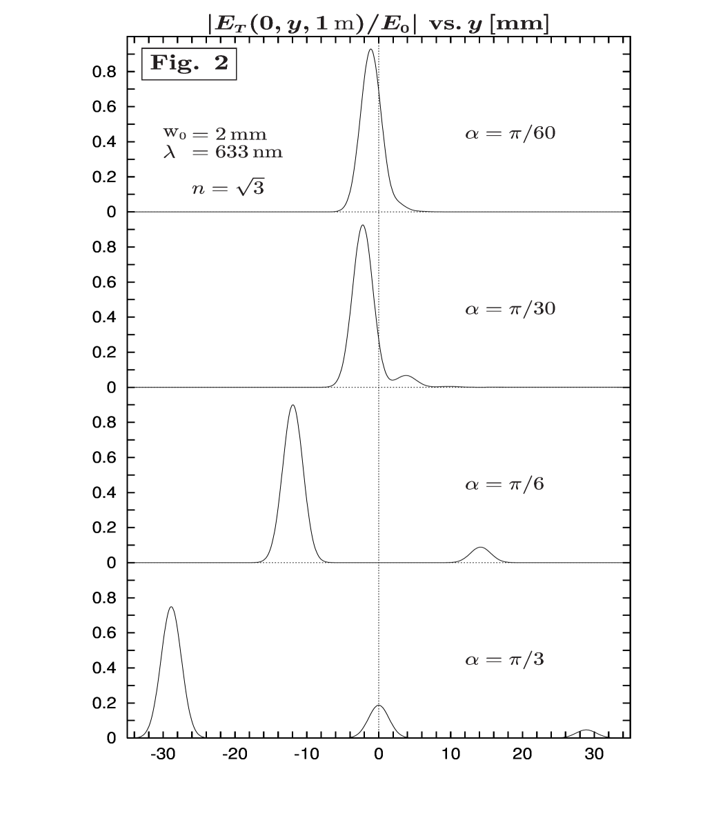
Figure 2: Numerical profiles of the modulus of the transmitted (normalized) electric field amplitude, for $x=0$ and $z=1\,\mbox{m}$, as a function of $y$. Four values of incident angles are shown. For increasing $\alpha$ the appearance of secondary peaks is seen.

This integral must be performed numerically. In Fig. 2, we plot the results for $|E_{\mbox{\tiny T}}/E_{\mbox{\tiny$0$}}|$ versus $y$ for four values of the incoming $\alpha$. The $x$-dependence is not plotted because it is the same as the incoming laser beam. We observe that for small $\alpha$ angles a single beam emerges. However, its peak is somewhat displaced w.r.t. the incoming beam (an effect of $T$). As $\alpha$ increases, evidence of a secondary beam is seen. For even high $\alpha$, this beam and others separate and we observe the effect of the incoherent limit of the transmission coefficient. Our curves are calculated directly from the full $T$, however they of course agree with those calculated from each appropriate transmission term. We exhibit only the first three terms in our plots.

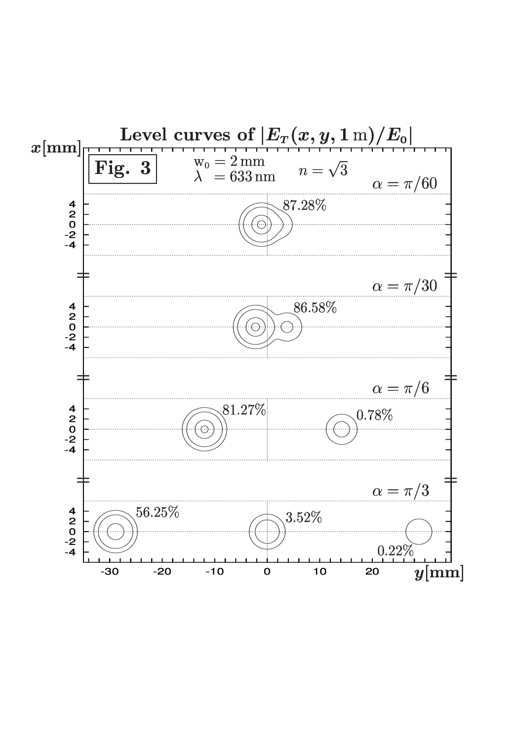
Figure 3: Planar view of the transmitted laser profiles displayed in Fig. 2. The outer curve corresponds to an intensity density of $0.01$ compared to the intensity of the incident peak, the second curve, where it exists, corresponds to $0.05$, the third to $0.4$ and the fourth to $0.8$. For each beam, we also give the numerical value of the integrated relative power $P_{rel}$ expressed in Eq. (16).

In Fig. 3 we plot these same results in a different manner suitable to direct experimental verification. We plot the $xy$-profile of each intensity for the four chosen $\alpha$. For these plots we have arbitrarily chosen $z=1\,\mbox{m}$, however, with the very small spreading in our simulation, the exact value of $z$ (below several meters) is irrelevant. All centers lie upon the $x$-axis as does the incoming beam profile. However the $y$ values depend upon $\alpha$. Another way of determining these $y$ values without going through a numerical calculation is by means of the SPM. We must now work with the individual transmission terms since the SPM only yields a single peak position $y$. The SPM applied to an expression which involves a sum of peaks yields only the mean value, normally not even coincident with any of the peaks. The SPM involves taking the derivative of the argument of the phase of a peaked function assuming it more relevant to the peak’s position compared to the modulus of the amplitude. Now the phase of our amplitudes take the form

$$e^{i\,[k_{y}y+f(k_{y})]}\,\,,$$

where $f(k_{y})$ is a function of $k_{y}$ (independent of any $y$ dependence). The function $f$ is calculated below. The SPM then says that the peak occurs where

$$y+\left.\frac{\mbox{d}f(k_{y})}{\mbox{d}k_{y}}\right|_{{}_{k_{y}=0}}=\,\,0\,\,.$$

Consider, the first leading transmission amplitude term $T_{\mbox{\tiny$1$}}T_{\mbox{\tiny$2$}}$, the phase is

$$(q_{z_{*}}-\,k_{z_{*}})(a+b)\,+\,(k_{z_{*}}-\,q_{z_{*}})\,a=(q_{z_{*}}-\,k_{z_{*}})\,b\,\,,$$

to which, we must add the plane wave phase $e^{ik_{y}y}$. Thus in this case, $f(k_{y})=(q_{z_{*}}-\,k_{z_{*}})\,b$. Before deriving w.r.t. $k_{y}$ this function, we recall that

$$q_{z_{*}}-\,k_{z_{*}}=k\,(n\cos\beta-\cos\alpha)+k_{y}\,(\sin\alpha-\tan\beta\cos\alpha)+\mbox{O}\left(k_{y}^{{}^{2}}\right)\,\,.$$

Thus,

$$\left.\frac{\mbox{d}f(k_{y})}{\mbox{d}k_{y}}\right|_{{}_{k_{y}=0}}=\,\,\frac{\sin(\alpha-\beta)}{\cos\beta}\,\,b\,\,.$$

Hence, for the first transmission term, the exit point is

$$y_{{}_{(1)}}[\,z_{*}=a+b\,]=-\,\frac{\sin(\alpha-\beta)}{\cos\beta}\,\,b\,\,.$$

The linear dependence upon $b$ is obvious because of geometry, indeed this expression and those below are also derivable by pure geometry. Repeating this procedure for the $m$-th peak ($m=1$ being the first), we must include the phase of $(R_{\mbox{\tiny$2$}}\widetilde{R}_{\mbox{\tiny$1$}})^{{}^{m-1}}$. This yields

$$y_{{}_{(m)}}[z_{*}=a+b]=-\,\left[\,\frac{\sin(\alpha-\beta)}{\cos\beta}-2\,(m-1)\,\tan\beta\cos\alpha\,\right]\,b\,\,.$$ (15)

In particular, the resulting values of the peaks for $\alpha=\pi/3$ are $y_{{}_{(m)}}=-\,(2-m)\,b\,/\,\sqrt{3}$. These agree very well with the center positions plotted in Fig. 3. The integrated power $P$ of each outgoing laser beam relative to the incoming beam power is given by

$$P_{rel}\approx\frac{\mbox{w}_{\mbox{\tiny$0$}}}{2\sqrt{2}\,\pi^{{}^{3/2}}}\,\int\,\mbox{d}y\,\,\left|\,\int\,\mbox{d}k_{y}\,\,T(0,k_{y})\,\exp\left[\,-\,\left(\,\frac{w_{\mbox{\tiny$0$}}^{\mbox{\tiny$2$}}}{4}+i\,\frac{z}{2\,k}\,\right)\,k_{y}^{{}^{2}}\,+\,i\,k_{y}\,y\right]\,\right|^{{}^{2}}\,\,.$$ (16)

For the calculation of the separate laser terms it is sufficient to use the following approxiamtions

$$|\,T_{\mbox{\tiny$1$}}T_{\mbox{\tiny$2$}}\,|\approx 4\,n\cos\alpha\,\cos\beta\,\mbox{\large$/$}(\cos\alpha+n\cos\beta)^{{}^{2}}\,\,\,\,\,\,\,\mbox{and}\,\,\,\,\,\,\,|\,R_{\mbox{\tiny$2$}}\widetilde{R}_{\mbox{\tiny$1$}}\,|\approx[\,(\cos\alpha-n\cos\beta)\mbox{\large$/$}(\cos\alpha+n\cos\beta)\,]^{{}^{2}}\,\,.$$

These are valid for small $k_{x,y}$. For example, for the particular case of an incident angle $\alpha=\pi/3$ and for a refractive index $n=\sqrt{3}$ (for which we have a diffusion angle $\beta=\pi/6$),

$$|\,T_{\mbox{\tiny$1$}}T_{\mbox{\tiny$2$}}\,|\approx 3/4\,\,\,\,\,\,\,\mbox{and}\,\,\,\,\,\,\,|\,R_{\mbox{\tiny$2$}}\widetilde{R}_{\mbox{\tiny$1$}}\,|\approx 1/4\,\,.$$

Hence the first three laser transmission beams have the following relative powers

$$P_{rel}(\pi/3)\approx\left(\,\frac{9}{16}\,,\,\frac{9}{16^{2}}\,,\,\frac{9}{16^{3}}\,\right)\,\,.$$

This result is in excellent agreement with the numerical results obtained from Eq.(16) and shown in Fig. 3.

VI. CONCLUSIONS

Our principal objective in this paper is to develop the formalism, conventions and approximations for the interaction of a gaussian laser beam with dielectric structures. We emphasize in particular the dominant role played by the momentum perpendicular to the dielectric block, $z_{*}$ component, and in general to any stratified dielectric system. This result draws a strong analogy with one-dimensional non-relativistic QM. Indeed we have noted in the text that our system corresponds to a QM well potential. The numerical and other calculations displayed in this work invite experimental confirmation. It is particularly interesting to note the conditions for coherence and incoherence in this study and compare them with those of one-dimensional QM. In QM we deal with time dependent wave packets and coherence requires the size of these wave packets to be large w.r.t. the well size. In this work the analogy is the separation in the $y$-variable of laser beams. For this optical study, coherence can be achieved not only by increasing the laser beam size w.r.t. the block depth $b$ so that overlap occurs between outgoing beams, but also by reducing the incident angle $\alpha$. This also leads to overlap of individual terms since the separation of the $y$ exit points is reduced, for any fixed laser size, by decreasing $\alpha$. We have calculated the various $y$ values for incoherence, both by the SPM and numerically and found complete agreement. They remain, of course, to be confirmed experimentally. We have also calculated, for various incident angles $\alpha$, the outgoing incoherent beam intensities and profiles.

A more complex and interesting situation occurs if we consider a dielectric slab cut diagonally, see the figure below.

The dielectric-air-dielectric system now mimics a potential barrier and in addition to diffusion we encounter tunneling. Tunneling still holds a number of theoretical conundrums notwithstanding its practical importance in technology such as in the tunneling microscope. It seems that technology has leap-frogged theory in this case. For example, there is still discussion in the literature about tunneling times[23, 24, 25] and possible superluminal velocities[13, 14]. Another theoretical conundrum is that for tunneling, our series calculation (two step method) yields a non convergent sum. Transmission seems always to be coherent, independent of the barrier/wave packet ratio. In the optical analogy, we pass from diffusion to tunneling by simply varying the incident angle. Tunneling occurs when $\varphi>\beta_{\mbox{\tiny critical}}=\arcsin(1/n)$.

Let us rapidly recall some of the contents of the previous sections. We started by representing the analytic function of a gaussian laser[22] and consequently extended our studies to 3-dimensional optics. We also extended this analysis to the laser beam within the dielectric. We then presented the optical analogy of a QM well problem and derived both by numerical and approximate analytic methods, SPM[20], the exit points from the dielectric block of the laser beam or beams for various incidence angles. We have calculated the intensities of the first few incoherent terms (beams) in the transition amplitude for a realistic experimental setup.

Finally, in this section, we have outlined a structure suitable for investigating both diffusion and tunneling again dependent upon the incident angle. Another more complex structure would be the optical analogy of twin barrier tunneling[16] which, as known, exhibits the extraordinary phenomena of resonant tunneling[9, 26]. These structures will be the subject of a subsequent report.

$\boldsymbol{T(k_{x},k_{y})}$
$\boldsymbol{\alpha=\pi/60}\,\,\bullet$	$\mbox{w}_{\mbox{\tiny$0$}}k_{x}\,:\,\,\,\,0\hskip 34.14322pt$	$\pm 2$	$\pm 4$	$\pm 6$
$\mbox{w}_{\mbox{\tiny$0$}}k_{y}\,:\,\,\,-6$	( 0.380 , 0.859 )	( 0.380 , 0.860 )	( 0.377 , 0.862 )	( 0.373 , 0.865 )
$-4$	( -0.475 , 0.788 )	( -0.476 , 0.788 )	( -0.478 , 0.786 )	( -0.482 , 0.782 )
$-2$	( -0.900 , 0.200 )	( -0.900 , 0.201 )	( -0.900 , 0.204 )	( -0.900 , 0.209 )
$\hskip 7.11317pt0$	( -0.356 , 0.868 )	( -0.355 , 0.868 )	( -0.352 , 0.869 )	( -0.347 , 0.869 )
$2$	( 0.686 , -0.592 )	( 0.687 , -0.592 )	( 0.689 , -0.590 )	( 0.693 , -0.586 )
$4$	( 0.921 , 0.248 )	( 0.920 , 0.249 )	( 0.919 , 0.252 )	( 0.917 , 0.256 )
$6$	( 0.060 , 0.892 )	( 0.059 , 0.892 )	( 0.057 , 0.893 )	( 0.051 , 0.894 )
$\boldsymbol{\alpha=\pi/30}\,\,\bullet$	$\mbox{w}_{\mbox{\tiny$0$}}k_{x}\,:\,\,\,\,0\hskip 34.14322pt$	$\pm 2$	$\pm 4$	$\pm 6$
$\mbox{w}_{\mbox{\tiny$0$}}k_{y}\,:\,\,\,-6$	( 0.345 , 0.904 )	( 0.344 , 0.904 )	( 0.341 , 0.904 )	( 0.337 , 0.905 )
$-4$	( -0.941 , -0.284 )	( -0.941 , -0.285 )	( -0.940 , -0.287 )	( -0.938 , -0.291 )
$-2$	( 0.813 , -0.572 )	( 0.814 , -0.571 )	( 0.815 , -0.570 )	( 0.817 , -0.565 )
$0$	( -0.056 , 0.998 )	( -0.056 , 0.998 )	( -0.059 , 0.998 )	( -0.063 , 0.997 )
$2$	( -0.746 , -0.664 )	( -0.746 , -0.664 )	( -0.744 , -0.666 )	( -0.742 , -0.670 )
$4$	( 0.978 , -0.170 )	( 0.978 , -0.169 )	( 0.979 , -0.167 )	( 0.980 , -0.163 )
$6$	( -0.469 , 0.862 )	( -0.470 , 0.862 )	( -0.473 , 0.861 )	( -0.477 , 0.859 )
$\boldsymbol{\alpha=\pi/6}\,\,\bullet$	$\mbox{w}_{\mbox{\tiny$0$}}k_{x}\,:\,\,\,\,0\hskip 34.14322pt$	$\pm 2$	$\pm 4$	$\pm 6$
$\mbox{w}_{\mbox{\tiny$0$}}k_{y}\,:\,\,\,-6$	( 0.161 , 0.942 )	( 0.160 , 0.942 )	( 0.158 , 0.943 )	( 0.153 , 0.945 )
$-4$	( 0.775 , 0.632 )	( 0.774 , 0.633 )	( 0.773 , 0.634 )	( 0.770 , 0.637 )
$-2$	( 0.946 , -0.024 )	( 0.946 , -0.023 )	( 0.946 , -0.020 )	( 0.947 , -0.016 )
$0$	( 0.689 , -0.518 )	( 0.689 , -0.518 )	( 0.691 , -0.516 )	( 0.693 , -0.511 )
$2$	( 0.301 , -0.764 )	( 0.302 , -0.764 )	( 0.305 , -0.763 )	( 0.310 , -0.761 )
$4$	( -0.134 , -0.832 )	( -0.134 , -0.832 )	( -0.131 , -0.833 )	( -0.126 , -0.836 )
$6$	( -0.624 , -0.674 )	( -0.623 , -0.675 )	( -0.622 , -0.678 )	( -0.629 , -0.681 )
$\boldsymbol{\alpha=\pi/3}\,\,\bullet$	$\mbox{w}_{\mbox{\tiny$0$}}k_{x}\,:\,\,\,\,0\hskip 34.14322pt$	$\pm 2$	$\pm 4$	$\pm 6$
$\mbox{w}_{\mbox{\tiny$0$}}k_{y}\,:\,\,\,-6$	( 0.397 , 0.480 )	( 0.397 , 0.480 )	( 0.395 , 0.482 )	( 0.393 , 0.484 )
$-4$	( 0.054 , -0.997 )	( 0.055 , -0.997 )	( 0.057 , -0.997 )	( 0.060 , -0.997 )
$-2$	( -0.401 , 0.464 )	( -0.401 , 0.464 )	( -0.402 , 0.462 )	( -0.404 , 0.461 )
$0$	( 0.670 , -0.472 )	( 0.671 , -0.472 )	( 0.671 , -0.470 )	( 0.672 , -0.466 )
$2$	( -0.665 , -0.345 )	( -0.665 , -0.346 )	( -0.664 , -0.348 )	( -0.664 , -0.350 )
$4$	( 0.500 , 0.393 )	( 0.500 , 0.393 )	( 0.499 , 0.395 )	( 0.496 , 0.397 )
$6$	( -0.051 , -0.983 )	( -0.051 , -0.983 )	( -0.049 , -0.983 )	( -0.046 , -0.984 )

Table 1: Values of the transmission amplitude, $(\mbox{Re}[T],\mbox{Im}[T])$, as a function of $k_{x}$ and $k_{y}$ for four incident angles, $\alpha=(\pi/60,\,\pi/30,\,\pi/6,\,\pi/3)$, for the chosen parameters $\mbox{w}_{\mbox{\tiny$0$}}=2\,\mbox{mm}$, $\lambda=633\,\mbox{nm}$, $n=\sqrt{3}$ and $b=5\,\mbox{cm}$. The dependence of $T$ upon $k_{x}$ is clearly very small.

Figure 1: Laser intensity profiles in air for two typical beam waists, $\mbox{w}_{\mbox{\tiny$0$}}=1\,\mbox{mm}$ and $\mbox{w}_{\mbox{\tiny$0$}}=2\,\mbox{mm}$, and for a wavelength value of $633\,\mbox{nm}$. The plot shows the wave number spread and the spatial laser width are complementar.

REFERENCES

- [1] M. Born and E. Wolf, Principles of optics, Cambridge UP, Cambridge (1999).
- [2] F. Abelés, Ann. de Physique 5, 596 (1950).
- [3] K. Ohta and H. Ishida, App. Opt. 29, 1952 (1990).
- [4] C. Cohen-Tannoudji, B. Diu and F. Laloë, Quantum mechanics, John Wiley & Sons, Paris (1977).
- [5] S. Menon, Q. Su, and R. Grobe, Phys. Rev. E 67, 046619 (2003).
- [6] A.B. Shvartsburg, V. Kuzmiak and G. Petite, Phys. Rep. 452, 33 (2007).
- [7] A. M. Steinberg, P.G. Kwiat, and R.Y. Chiao, Phys. Rev. Lett. 71, 708 (1993).
- [8] S. Longhi, M. Marano, P. Laporta, and M. Belmonte, Phys. Rev E 64, 055602 (2001)
- [9] A. Haibel, G. Nimtz, and A.A. Stahlhofen, Phys. Rev. E 63, 047601 (2001).
- [10] S. Longhi, M. Marano, P. Laporta, and M. Belmonte, Phys. Rev E 64, 055602 (2001)
- [11] G. Nimtz, A. Haibel and R.M. Vetter, Phys. Rev. E 66, 037602 (2002).
- [12] E. Recami, J. Mod. Opt. 51, 913 (2004)
- [13] V. S. Olkhovsky, E. Recami and J. Jakiel, Phys. Rep. 398, 133 (2004).
- [14] H. Winful, Phys. Rep. 436, 1 (2006).
- [15] A. Bernardini, S. De Leo and P. Rotelli, Mod. Phys. Lett. A 19, 2717 (2004).
- [16] S. De Leo and P. Rotelli, Phys. Lett. A 342, 294 (2005).
- [17] S. De Leo and P. Rotelli, Eur. Phys. J. C 46, 551 (2006).
- [18] S. De Leo and P. Rotelli, J. Opt. A 10, 115001 (2008).
- [19] E. Wigner, Phys. Rev. 98, 145 (1955)
- [20] N. Bleistein and R. Handelsman, Asymptotic Expansions of Integrals, Dover, New York (1975).
- [21] M. J. Weber, Handbook of Lasers, CRC Press LLC, USA (2001).
- [22] J. Enderlein and F. Pampaloni, J. Opt. Soc. Am. A, 21, 1553 (2004).
- [23] T. E. Hartman, J. Appl. Phys. 33, 3427 (1962).
- [24] E.H. Hauge and J.A. Stovneng, Rev. Mod. Phys. 61, 917 (1989).
- [25] V. S. Olkhovsky and E. Recami, Phys. Rep. 214, 339 (1992).
- [26] S. Hayashi, H. Kurokawa, and H. Oga, Opt. Rev. 6, 204 (1990).