Symbolic and Asynchronous Semantics
via Normalized Coalgebras*

Abstract.

The operational semantics of interactive systems is usually described by labeled transition systems. Abstract semantics (that is defined in terms of bisimilarity) is characterized by the final morphism in some category of coalgebras. Since the behaviour of interactive systems is for many reasons infinite, symbolic semantics were introduced as a mean to define smaller, possibly finite, transition systems, by employing symbolic actions and avoiding some sources of infiniteness. Unfortunately, symbolic bisimilarity has a different shape with respect to ordinary bisimilarity, and thus the standard coalgebraic characterization does not work. In this paper, we introduce its coalgebraic models.

We will use as motivating examples two asynchronous formalisms: open Petri nets and asynchronous pi-calculus. Indeed, as we have shown in a previous paper, asynchronous bisimilarity can be seen as an instance of symbolic bisimilarity.

Introduction

A compositional interactive system is usually defined as a labelled transition system (lts) where states are equipped with an algebraic structure. Abstract semantics is often defined as bisimilarity. Then a key property is that “bisimilarity is a congruence”, i.e., that abstract semantics respects the algebraic operations.

Universal Coalgebra [40] provides a categorical framework where the behaviour of dynamical systems can be characterized as final semantics. More precisely, if ${\bf Coalg_{B}}$ (i.e., the category of ${\bf B}$-coalgebras and ${\bf B}$-cohomomorphisms for a certain endofunctor ${\bf B}$) has a final object, then the behavior of a ${\bf B}$-coalgebra is defined as a final morphism. Intuitively, a final object is a universe of abstract behaviors and a final morphism is a function mapping each system in its abstract behavior. Ordinary ltss can be represented as coalgebras for a suitable functor. Then, two states are bisimilar if and only if they are identified by a final morphism. The image of a certain lts through a final morphism is its minimal representative (with respect to bisimilarity), which in the finite case can be computed via the partition refinement algorithm [26]. Existence and construction of the minimal transition system is a key property of the coalgebraic approach. It allows to model check efficiently for several properties by eliminating redundant states once and for all. In fact most model checking logics are adequate, namely either a formula holds in both the given system and in its minimal representative or it does not hold in both of them.

When bisimilarity is not a congruence, the abstract semantics is defined either as the largest congruence contained in bisimilarity [31] or as the largest bisimulation that is also a congruence [36]. In this paper we focus on the latter and we call it saturated bisimilarity ($\sim^{S}$). Indeed it coincides with ordinary bisimilarity on the saturated transition system that is obtained from the original lts by adding the transition $p\stackrel{{\scriptstyle c,a}}{{\mathord{\smash{-}}\mkern-6.0mu\cleaders\hbox{$\mkern-2.0mu\mathord{\smash{-}}\mkern-2.0mu$}\hfill\mkern-6.0mu\mathord{\rightarrow}}}q$, for every context $c$, whenever $c(p)\stackrel{{\scriptstyle a}}{{\mathord{\smash{-}}\mkern-6.0mu\cleaders\hbox{$\mkern-2.0mu\mathord{\smash{-}}\mkern-2.0mu$}\hfill\mkern-6.0mu\mathord{\rightarrow}}}q$.

Many interesting abstract semantics are defined in this way. For example, since late and early bisimilarity of the $\pi$-calculus [33] are not preserved under substitution (and thus under input prefixes), in [41] Sangiorgi introduces open bisimilarity as the largest bisimulation on $\pi$-calculus agents which is closed under substitutions. Other noteworthy examples are asynchronous $\pi$-calculus [1, 25], mobile ambients calculus [12, 30] and (explicit [43]) fusion calculus [37]. The definition of saturated bisimilarity as ordinary bisimilarity on the saturated lts often makes infinite the portion of lts reachable by any nontrivial agent and, in any case, is very inefficient, since it introduces a large number of additional states and transitions. Inspired by Hennessy and Lin [24], who introduced a symbolic semantics of value passing calculi, Sangiorgi defines in [41] a symbolic transition system and symbolic bisimilarity that efficiently characterizes open bisimilarity. After this, many formalisms have been equipped with a symbolic semantics.

In [8], we have introduced a general model that describes at an abstract level both saturated and symbolic semantics. In this abstract setting, a symbolic transition $p\stackrel{{\scriptstyle c,\alpha}}{{\mathord{\smash{-}}\mkern-6.0mu\cleaders\hbox{$\mkern-2.0mu\mathord{\smash{-}}\mkern-2.0mu$}\hfill\mkern-6.0mu\mathord{\rightarrow}}}_{\beta}p^{\prime}$ means that $c(p)\stackrel{{\scriptstyle\alpha}}{{\mathord{\smash{-}}\mkern-6.0mu\cleaders\hbox{$\mkern-2.0mu\mathord{\smash{-}}\mkern-2.0mu$}\hfill\mkern-6.0mu\mathord{\rightarrow}}}p^{\prime}$ and $c$ is a smallest context that allows $p$ to performs such a transition. Moreover, a certain derivation relation $\vdash$ amongst the transitions of a system is defined: $p\stackrel{{\scriptstyle c_{1},\alpha_{1}}}{{\mathord{\smash{-}}\mkern-6.0mu\cleaders\hbox{$\mkern-2.0mu\mathord{\smash{-}}\mkern-2.0mu$}\hfill\mkern-6.0mu\mathord{\rightarrow}}}p_{1}\vdash p\stackrel{{\scriptstyle c_{2},\alpha_{2}}}{{\mathord{\smash{-}}\mkern-6.0mu\cleaders\hbox{$\mkern-2.0mu\mathord{\smash{-}}\mkern-2.0mu$}\hfill\mkern-6.0mu\mathord{\rightarrow}}}p_{2}$ means that the latter transition is a logical consequence of the former. In this way, if all and only the saturated transitions are logical consequences of symbolic transitions, then saturated bisimilarity can be retrieved via the symbolic lts.

Unfortunately, the ordinary bisimilarity over the symbolic transition system differs from saturated bisimilarity. Symbolic bisimilarity is thus defined with an asymmetric shape: in the bisimulation game, when a player proposes a transition, the opponent can answer with a move with a different label. For example in the open $\pi$-calculus, a transition $p\stackrel{{\scriptstyle[a=b],\tau}}{{\mathord{\smash{-}}\mkern-6.0mu\cleaders\hbox{$\mkern-2.0mu\mathord{\smash{-}}\mkern-2.0mu$}\hfill\mkern-6.0mu\mathord{\rightarrow}}}p^{\prime}$ can be matched by $q\stackrel{{\scriptstyle\tau}}{{\mathord{\smash{-}}\mkern-6.0mu\cleaders\hbox{$\mkern-2.0mu\mathord{\smash{-}}\mkern-2.0mu$}\hfill\mkern-6.0mu\mathord{\rightarrow}}}q^{\prime}$. Moreover, the bisimulation game does not restart from $p^{\prime}$ and $q^{\prime}$, but from $p^{\prime}$ and $q^{\prime}\{b/a\}$.

For this reason, ordinary coalgebras fail to characterize symbolic bisimilarity. Here, we provide coalgebraic models for it by relying on the framework of [8].

Consider the example of open bisimilarity discussed above. The fact that open bisimulation does not relate the arriving states $p^{\prime}$ and $q^{\prime}$, but $p^{\prime}$ and $q^{\prime}\{b/a\}$, forces us to look for models equipped with an algebraic structure. In [42], bialgebras are introduced as a both algebraic and coalgebraic model, while an alternative approach based on structured coalgebras, i.e., on coalgebras in categories of algebras, is presented in [13]. In this paper we adopt the latter and we introduce ${\bf Coalg_{{\bf H}}}$ (Section 6), a category of structured coalgebras where the saturated transition system can be naively modeled in such a way that $\sim^{S}$ coincides with the kernel of a final morphism. Then, we focus only on those ${\bf H}$-coalgebras whose sets of transitions are closed w.r.t. the derivation relation $\vdash$. These form the category of saturated coalgebras ${\bf Coalg_{{\bf{S_{T}}}}}$ (Section 7.1) that is (isomorphic to) a covariety of ${\bf Coalg_{{\bf H}}}$. Thus, it has a final object and bisimilarity coincides with the one in ${\bf Coalg_{{\bf H}}}$.

In order to characterize symbolic bisimilarity, we introduce the notions of redundant transition and semantically redundant transition. Intuitively, a transition $p\stackrel{{\scriptstyle c_{2},\alpha_{2}}}{{\mathord{\smash{-}}\mkern-6.0mu\cleaders\hbox{$\mkern-2.0mu\mathord{\smash{-}}\mkern-2.0mu$}\hfill\mkern-6.0mu\mathord{\rightarrow}}}q$ is redundant if there exists another transition $p\stackrel{{\scriptstyle c_{1},\alpha_{1}}}{{\mathord{\smash{-}}\mkern-6.0mu\cleaders\hbox{$\mkern-2.0mu\mathord{\smash{-}}\mkern-2.0mu$}\hfill\mkern-6.0mu\mathord{\rightarrow}}}p_{1}$ that logically implies it, that is $p\stackrel{{\scriptstyle c_{1},\alpha_{1}}}{{\mathord{\smash{-}}\mkern-6.0mu\cleaders\hbox{$\mkern-2.0mu\mathord{\smash{-}}\mkern-2.0mu$}\hfill\mkern-6.0mu\mathord{\rightarrow}}}p_{1}\vdash p\stackrel{{\scriptstyle c_{2},\alpha_{2}}}{{\mathord{\smash{-}}\mkern-6.0mu\cleaders\hbox{$\mkern-2.0mu\mathord{\smash{-}}\mkern-2.0mu$}\hfill\mkern-6.0mu\mathord{\rightarrow}}}q$; it is semantically redundant, if it is “redundant up to bisimilarity”, i.e., $p\stackrel{{\scriptstyle c_{1},\alpha_{1}}}{{\mathord{\smash{-}}\mkern-6.0mu\cleaders\hbox{$\mkern-2.0mu\mathord{\smash{-}}\mkern-2.0mu$}\hfill\mkern-6.0mu\mathord{\rightarrow}}}p_{1}\vdash p\stackrel{{\scriptstyle c_{2},\alpha_{2}}}{{\mathord{\smash{-}}\mkern-6.0mu\cleaders\hbox{$\mkern-2.0mu\mathord{\smash{-}}\mkern-2.0mu$}\hfill\mkern-6.0mu\mathord{\rightarrow}}}p_{2}$ and $q$ is bisimilar to $p_{2}$. Now, in order to retrieve saturated bisimilarity by disregarding redundant transitions, we have to remove from the saturated transition system not only all the redundant transitions, but also the semantically redundant ones. This is done in the category of normalized coalgebras ${\bf Coalg_{{\bf N_{T}}}}$ (Section 7.2). These are defined as coalgebras without redundant transitions. Thus, by definition, a final coalgebra in ${\bf Coalg_{{\bf N_{T}}}}$ has no semantically redundant transitions.

We prove that ${\bf Coalg_{{\bf{S_{T}}}}}$ and ${\bf Coalg_{{\bf N_{T}}}}$ are isomorphic (Section 7.3). This means that a final morphism in the latter category still characterizes $\sim^{S}$, but with two important differences w.r.t. ${\bf Coalg_{{\bf{S_{T}}}}}$. First of all, in a final ${\bf N_{T}}$-coalgebra, there are no semantically redundant transitions. Intuitively, a final ${\bf N_{T}}$-coalgebra is a universe of abstract symbolic behaviours and a final morphism maps each system in its abstract symbolic behaviour. Secondly, minimization in ${\bf Coalg_{{\bf N_{T}}}}$ is feasible, while in ${\bf Coalg_{{\bf{S_{T}}}}}$ is not, because saturated coalgebras have all the redundant transitions. Minimizing in ${\bf Coalg_{{\bf N_{T}}}}$ coincides with a symbolic minimization algorithm that we have introduced in [10] (Section 8). The algorithm shows another peculiarity of normalized coalgebras: minimization relies on the algebraic structure. Since in bialgebras bisimilarity abstracts away from this, we can conclude that our normalized coalgebras are not bialgebras. This is the reason why we work with structured coalgebras.

As motivating examples we will show open Petri nets [27, 3] (Section 2) and asynchronous $\pi$-calculus [25, 1] (Section 1). In [8], we have shown that asynchronous bisimilarity [1] is an instance of symbolic bisimilarity. Indeed, in the definition of asynchronous bisimulation, the input transition $p\stackrel{{\scriptstyle a(b)}}{{\mathord{\smash{-}}\mkern-6.0mu\cleaders\hbox{$\mkern-2.0mu\mathord{\smash{-}}\mkern-2.0mu$}\hfill\mkern-6.0mu\mathord{\rightarrow}}}p^{\prime}$ can be matched either by $q\stackrel{{\scriptstyle a(b)}}{{\mathord{\smash{-}}\mkern-6.0mu\cleaders\hbox{$\mkern-2.0mu\mathord{\smash{-}}\mkern-2.0mu$}\hfill\mkern-6.0mu\mathord{\rightarrow}}}q^{\prime}$ or by $q\stackrel{{\scriptstyle\tau}}{{\mathord{\smash{-}}\mkern-6.0mu\cleaders\hbox{$\mkern-2.0mu\mathord{\smash{-}}\mkern-2.0mu$}\hfill\mkern-6.0mu\mathord{\rightarrow}}}q^{\prime}$. In the latter case, the bisimulation game does not restart from $p^{\prime}$ and $q^{\prime}$ but from $p^{\prime}$ and $q^{\prime}|\overline{a}b$. Thus our framework will provide, as lateral result, also a coalgebraic model for asynchronous bisimilarity that, as far as we know, has never been proposed so far.

In Section 4 and 5 we report the framework of [8] and we recall the basic notions on (structured) coalgebras. In Section 3 we introduce a further example aimed at clarifying the whole framework (by avoiding all the technical details of open Petri nets and asynchronous $\pi$). All proofs are in Appendix.

Previous works.

Our work relies on the framework introduced in [8] and on the minimization algorithm in [10]. In this work we focus on the coalgebraic characterization of them that appeared in [9]. The present paper extends [9] by (1) introducing the example of asynchronous $\pi$-calculus, (2) by adding all the proofs, (3) by explaining in full details the relationship with the minimization algorithm in [10]. Normalized coalgebras have been previously introduced in [7] for giving a coalgebraic characterization of the theory of reactive systems by Leifer and Milner [29].

1. Asynchronous $\pi$-calculus

Asynchronous $\pi$-calculus has been introduced in [25] for modeling distributed systems interacting via asynchronous message passing. Differently from the synchronous case, where messages are sent and received at the same time, in the asynchronous communication, messages are sent and travel through some media until they reach the destination. Therefore sending messages is non blocking (i.e., a process can send messages even if the receiver is not ready to receive), while receiving is blocking (processes must wait until the message has arrived). This asymmetry is reflected on the observations: since sending is non blocking, receiving is unobservable.

In this section, we introduce asynchronous $\pi$-calculus and two definitions of bisimilarity ($\sim^{1}$ and $\sim^{a}$) that, as proved in [1], coincide. In Section 4, we will show that the first is an instance of our general definition of saturated bisimilarity (Definition 4.1) while the second of symbolic bisimilarity (Definition 4.2).

Let $\mathcal{N}$ be a set of names (ranged over by $a,b,c\dots$) with $\tau\notin\mbox{$\mathcal{N}$}$. The set of $\pi$-processes is defined by the following grammar:

$$p::=\overline{a}b,\;\;p_{1}|p_{2},\;\;\nu a.p,\;\;!g,\;\;m\;\;\;\;\;\;\;m::=\mathbf{0},\;\;\alpha.p,\;\;m_{1}+m_{2}\;\;\;\;\;\;\;\alpha::=a(b),\;\;\tau$$

The main difference with the ordinary $\pi$-calculus [33] is that here output prefixes are missing. The occurrence of an unguarded $\bar{a}b$ can be thought of as message $b$ that is available on some communication media named $a$. This message is received whenever it disappears, i.e., it is consumed by some process performing an input. Thus the action of sending happens when $\bar{a}b$ becomes unguarded.

Considering $a(b).p$ and $\nu b.p$, the occurrences of $b$ in $p$ are bound. An occurrence of a name in a process is free, if it is not bound. The set of free names of $p$ (denoted by $\mathrm{fn}(p)$) is the set of names that have a free occurrence in the process $p$. The process $p$ is $\alpha$-equivalent to $q$ (written $p\equiv_{\alpha}q$), if they are equivalent up to $\alpha$-renaming of bound occurrences of names. The operational semantics of $\pi$-calculus is a transition system labeled on actions $Act=\{a(b),\overline{a}b,\overline{{a}}({b}),\tau\mid a,b\in\mbox{$\mathcal{N}$}\}$ (ranged over by $\mu$) where $b$ is a bound name (written $b\in\mathrm{bn}(\mu)$) in $a(b)$ and $\overline{{a}}({b})$. In all the other cases $a$ and $b$ are free in $\mu$ ($a,b\in\mathrm{fn}(\mu)$). By $\mathrm{nm}(\mu)$ we denote the set of both free and bound names of $\mu$.

(tau) $\tau.p\stackrel{{\scriptstyle\tau}}{{\mathord{\smash{-}}\mkern-6.0mu\cleaders\hbox{$\mkern-2.0mu\mathord{\smash{-}}\mkern-2.0mu$}\hfill\mkern-6.0mu\mathord{\rightarrow}}}p$	(in) $a(b).p\stackrel{{\scriptstyle a(c)}}{{\mathord{\smash{-}}\mkern-6.0mu\cleaders\hbox{$\mkern-2.0mu\mathord{\smash{-}}\mkern-2.0mu$}\hfill\mkern-6.0mu\mathord{\rightarrow}}}p\{^{c}/_{b}\}$	(out) $\overline{a}b\stackrel{{\scriptstyle\overline{a}b}}{{\mathord{\smash{-}}\mkern-6.0mu\cleaders\hbox{$\mkern-2.0mu\mathord{\smash{-}}\mkern-2.0mu$}\hfill\mkern-6.0mu\mathord{\rightarrow}}}\mathbf{0}$
(com) $\frac{\displaystyle p\stackrel{{\scriptstyle\overline{a}b}}{{\mathord{\smash{-}}\mkern-6.0mu\cleaders\hbox{$\mkern-2.0mu\mathord{\smash{-}}\mkern-2.0mu$}\hfill\mkern-6.0mu\mathord{\rightarrow}}}p^{\prime}\quad q\stackrel{{\scriptstyle a(b)}}{{\mathord{\smash{-}}\mkern-6.0mu\cleaders\hbox{$\mkern-2.0mu\mathord{\smash{-}}\mkern-2.0mu$}\hfill\mkern-6.0mu\mathord{\rightarrow}}}q^{\prime}}{\displaystyle p|q\stackrel{{\scriptstyle\tau}}{{\mathord{\smash{-}}\mkern-6.0mu\cleaders\hbox{$\mkern-2.0mu\mathord{\smash{-}}\mkern-2.0mu$}\hfill\mkern-6.0mu\mathord{\rightarrow}}}p^{\prime}|q^{\prime}}$	(sum) $\frac{\displaystyle p\stackrel{{\scriptstyle\mu}}{{\mathord{\smash{-}}\mkern-6.0mu\cleaders\hbox{$\mkern-2.0mu\mathord{\smash{-}}\mkern-2.0mu$}\hfill\mkern-6.0mu\mathord{\rightarrow}}}p^{\prime}}{\displaystyle p+q\stackrel{{\scriptstyle\mu}}{{\mathord{\smash{-}}\mkern-6.0mu\cleaders\hbox{$\mkern-2.0mu\mathord{\smash{-}}\mkern-2.0mu$}\hfill\mkern-6.0mu\mathord{\rightarrow}}}p^{\prime}}$	(par) $\frac{\displaystyle p\stackrel{{\scriptstyle\mu}}{{\mathord{\smash{-}}\mkern-6.0mu\cleaders\hbox{$\mkern-2.0mu\mathord{\smash{-}}\mkern-2.0mu$}\hfill\mkern-6.0mu\mathord{\rightarrow}}}p^{\prime}}{\displaystyle p|q\stackrel{{\scriptstyle\mu}}{{\mathord{\smash{-}}\mkern-6.0mu\cleaders\hbox{$\mkern-2.0mu\mathord{\smash{-}}\mkern-2.0mu$}\hfill\mkern-6.0mu\mathord{\rightarrow}}}p^{\prime}|q}$ $\mathrm{bn}(\mu)\cap\mathrm{fn}(q)=\emptyset$
(opn) $\frac{\displaystyle p\stackrel{{\scriptstyle\overline{a}b}}{{\mathord{\smash{-}}\mkern-6.0mu\cleaders\hbox{$\mkern-2.0mu\mathord{\smash{-}}\mkern-2.0mu$}\hfill\mkern-6.0mu\mathord{\rightarrow}}}p^{\prime}}{\displaystyle\nu b.p\stackrel{{\scriptstyle\overline{{a}}({b})}}{{\mathord{\smash{-}}\mkern-6.0mu\cleaders\hbox{$\mkern-2.0mu\mathord{\smash{-}}\mkern-2.0mu$}\hfill\mkern-6.0mu\mathord{\rightarrow}}}p^{\prime}}$ $b\neq a$	(rep) $\frac{\displaystyle m|!m\stackrel{{\scriptstyle\mu}}{{\mathord{\smash{-}}\mkern-6.0mu\cleaders\hbox{$\mkern-2.0mu\mathord{\smash{-}}\mkern-2.0mu$}\hfill\mkern-6.0mu\mathord{\rightarrow}}}q}{\displaystyle!m\stackrel{{\scriptstyle\mu}}{{\mathord{\smash{-}}\mkern-6.0mu\cleaders\hbox{$\mkern-2.0mu\mathord{\smash{-}}\mkern-2.0mu$}\hfill\mkern-6.0mu\mathord{\rightarrow}}}q}$	(cls) $\frac{\displaystyle p\stackrel{{\scriptstyle\overline{{a}}({b})}}{{\mathord{\smash{-}}\mkern-6.0mu\cleaders\hbox{$\mkern-2.0mu\mathord{\smash{-}}\mkern-2.0mu$}\hfill\mkern-6.0mu\mathord{\rightarrow}}}p^{\prime}\quad q\stackrel{{\scriptstyle a(b)}}{{\mathord{\smash{-}}\mkern-6.0mu\cleaders\hbox{$\mkern-2.0mu\mathord{\smash{-}}\mkern-2.0mu$}\hfill\mkern-6.0mu\mathord{\rightarrow}}}q^{\prime}}{\displaystyle p|q\stackrel{{\scriptstyle\tau}}{{\mathord{\smash{-}}\mkern-6.0mu\cleaders\hbox{$\mkern-2.0mu\mathord{\smash{-}}\mkern-2.0mu$}\hfill\mkern-6.0mu\mathord{\rightarrow}}}\nu b.p^{\prime}|q^{\prime}}$$b\notin\mathrm{fn}(q)$
(res) $\frac{\displaystyle p\stackrel{{\scriptstyle\mu}}{{\mathord{\smash{-}}\mkern-6.0mu\cleaders\hbox{$\mkern-2.0mu\mathord{\smash{-}}\mkern-2.0mu$}\hfill\mkern-6.0mu\mathord{\rightarrow}}}p^{\prime}}{\displaystyle\nu b.p\stackrel{{\scriptstyle\mu}}{{\mathord{\smash{-}}\mkern-6.0mu\cleaders\hbox{$\mkern-2.0mu\mathord{\smash{-}}\mkern-2.0mu$}\hfill\mkern-6.0mu\mathord{\rightarrow}}}\nu b.p^{\prime}}$ $b\notin\mathrm{nm}(\mu)$

Table 1. Operational semantics of asynchronous $\pi$-calculus.

The labeled transition system (lts) is inductively defined by the rules in Table 1, where we have omitted the symmetric version of the rules sum, par, com and cls and where we consider processes up to $\alpha$-equivalence, i.e., we have implicitly assumed the rule

$$\displaystyle{\hbox{\hskip 27.12839pt\vbox{\hbox{\hskip-27.12839pt\hbox{\hbox{$\displaystyle\displaystyle{p\stackrel{{\scriptstyle\mu}}{{\mathord{\smash{-}}\mkern-6.0mu\cleaders\hbox{$\displaystyle\mkern-2.0mu\mathord{\smash{-}}\mkern-2.0mu$}\hfill\mkern-6.0mu\mathord{\rightarrow}}}q\;\;\;p\equiv_{\alpha}p^{\prime}}$}}}\vbox{}}}\over\hbox{\hskip 10.86166pt\vbox{\vbox{}\hbox{\hskip-10.86165pt\hbox{\hbox{$\displaystyle\displaystyle{p^{\prime}\stackrel{{\scriptstyle\mu}}{{\mathord{\smash{-}}\mkern-6.0mu\cleaders\hbox{$\displaystyle\mkern-2.0mu\mathord{\smash{-}}\mkern-2.0mu$}\hfill\mkern-6.0mu\mathord{\rightarrow}}}q}$}}}}}}$$.

The main difference with the synchronous case is in the notion of observation. Since sending messages is non-blocking, then an external observer can just send messages to a system without knowing if they will be received or not. For this reason the receiving action is not observable and the abstract semantics is defined disregarding input transitions.

As in the case of the standard $\pi$-calculus, in the bisimulation game we have to take care of the bound names in output actions. Indeed, when a process $p\stackrel{{\scriptstyle\overline{{a}}({b})}}{{\mathord{\smash{-}}\mkern-6.0mu\cleaders\hbox{$\mkern-2.0mu\mathord{\smash{-}}\mkern-2.0mu$}\hfill\mkern-6.0mu\mathord{\rightarrow}}}p^{\prime}$, the name $b$ is initially bound in $p$ and becomes free in $p^{\prime}$. Thus, in order to avoid name-clashes, in the bisimulation game when comparing $p$ and $q$, we require $b$ to be fresh, namely, different from all the free names of $p$ and $q$. In the following definitions, by “$\mathrm{bn}(\mu)$ is fresh” we mean that if $\mu$ has a bound name, then it is fresh.

[$o\tau$-Bisimilarity] A symmetric relation $R$ is an $o\tau$-bisimulation iff, whenever $pRq$:

1. if $p\stackrel{{\scriptstyle\mu}}{{\mathord{\smash{-}}\mkern-6.0mu\cleaders\hbox{$\mkern-2.0mu\mathord{\smash{-}}\mkern-2.0mu$}\hfill\mkern-6.0mu\mathord{\rightarrow}}}p^{\prime}$ where $\mu$ is not an input action and $\mathrm{bn}(\mu)$ is fresh, then $\exists q^{\prime}$ such that $q\stackrel{{\scriptstyle\mu}}{{\mathord{\smash{-}}\mkern-6.0mu\cleaders\hbox{$\mkern-2.0mu\mathord{\smash{-}}\mkern-2.0mu$}\hfill\mkern-6.0mu\mathord{\rightarrow}}}q^{\prime}$ and $p^{\prime}Rq^{\prime}$.

We say that $p$ and $q$ are $o\tau$-bisimilar (written $p\sim^{o\tau}q$) if and only if there exists an $o\tau$-bisimulation relating them.

Note that $a(x).\overline{y}x\sim^{o\tau}a(x).\overline{d}x$, even if the two processes are really different when they are put in parallel with a process $\overline{a}b$. In order to obtain an abstract semantics preserved under parallel composition, we proceed analogously to saturated bisimilarity (that we will show in Definition 4.1), i.e., at any step of the bisimulation we put the process in parallel with all possible outputs. [1-Bisimilarity] A symmetric relation $R$ is an 1-bisimulation iff, $\forall\overline{a}b$, whenever $pRq$,

1. if $\overline{a}b|p\stackrel{{\scriptstyle\mu}}{{\mathord{\smash{-}}\mkern-6.0mu\cleaders\hbox{$\mkern-2.0mu\mathord{\smash{-}}\mkern-2.0mu$}\hfill\mkern-6.0mu\mathord{\rightarrow}}}p^{\prime}$ where $\mu$ is not an input action and $\mathrm{bn}(\mu)$ is fresh, then $\exists q^{\prime}$ such that $\overline{a}b|q\stackrel{{\scriptstyle\mu}}{{\mathord{\smash{-}}\mkern-6.0mu\cleaders\hbox{$\mkern-2.0mu\mathord{\smash{-}}\mkern-2.0mu$}\hfill\mkern-6.0mu\mathord{\rightarrow}}}q^{\prime}$ and $p^{\prime}Rq^{\prime}$.

We say that $p$ and $q$ are $1$-bisimilar (written $p\sim^{1}q$) if and only if there exists an $1$-bisimulation relating them.

The above definition is not very efficient since it considers a quantification over all possible output in parallel. Instead of considering all possible output contexts, we could also consider the input actions. This leads to the following notion of syntactic bisimulation.

[Syntactic Bisimilarity] A symmetric relation $R$ is a syntactic bisimulation iff, whenever $pRq$:

1. if $p\stackrel{{\scriptstyle\mu}}{{\mathord{\smash{-}}\mkern-6.0mu\cleaders\hbox{$\mkern-2.0mu\mathord{\smash{-}}\mkern-2.0mu$}\hfill\mkern-6.0mu\mathord{\rightarrow}}}p^{\prime}$ where $\mathrm{bn}(\mu)$ is fresh, then $\exists q^{\prime}$ such that $q\stackrel{{\scriptstyle\mu}}{{\mathord{\smash{-}}\mkern-6.0mu\cleaders\hbox{$\mkern-2.0mu\mathord{\smash{-}}\mkern-2.0mu$}\hfill\mkern-6.0mu\mathord{\rightarrow}}}q^{\prime}$ and $p^{\prime}Rq^{\prime}$.

We say that $p$ and $q$ are syntactic bisimilar (written $p\sim^{SYN}q$) if and only if there exists a syntactic bisimulation relating them. Note that syntactic bisimilarity is strictly included into $1$-bisimilarity. Indeed,

$$\tau+a(b).\overline{a}b\sim^{1}\tau\text{, but }\tau+a(b).\overline{a}b\not\sim^{SYN}\tau\text{.}$$

The former equivalence can be understood by observing that both processes can perform a $\tau$ transition in any possible context and, when inserted into the context $-|\overline{a}x$, both can perform a $\tau$ transition going into $\overline{a}x$. More generally, it holds that for all processes $p\sim^{1}q\sim^{1}r$:

$$\tau.p+a(b).(\overline{a}b|q)\sim^{1}\tau.r$$

For instance, by taking $q=r=\mathbf{0}$ and $p=\nu y.\overline{y}a$ (that is $1$-bisimilar to $\mathbf{0}$, since both cannot move), we have that $\tau.\nu y.\overline{y}a+a(b).\overline{a}b\sim^{1}\tau.\mathbf{0}$. Their ltss are shown in Figure 1(A).

In order to efficiently characterize $\sim^{1}$, without considering all possible contexts, we have to properly tackle the input transitions.

[Asynchronous Bisimilarity] A symmetric relation $R$ is an asynchronous bisimulation iff whenever $pRq$,

1. if $p\stackrel{{\scriptstyle\mu}}{{\mathord{\smash{-}}\mkern-6.0mu\cleaders\hbox{$\mkern-2.0mu\mathord{\smash{-}}\mkern-2.0mu$}\hfill\mkern-6.0mu\mathord{\rightarrow}}}p^{\prime}$ where $\mu$ is not an input action and $\mathrm{bn}(\mu)$ is fresh, then $\exists q^{\prime}$ such that $q\stackrel{{\scriptstyle\mu}}{{\mathord{\smash{-}}\mkern-6.0mu\cleaders\hbox{$\mkern-2.0mu\mathord{\smash{-}}\mkern-2.0mu$}\hfill\mkern-6.0mu\mathord{\rightarrow}}}q^{\prime}$ and $p^{\prime}Rq^{\prime}$,

2. if $p\stackrel{{\scriptstyle a(b)}}{{\mathord{\smash{-}}\mkern-6.0mu\cleaders\hbox{$\mkern-2.0mu\mathord{\smash{-}}\mkern-2.0mu$}\hfill\mkern-6.0mu\mathord{\rightarrow}}}p^{\prime}$, then $\exists q^{\prime}$ such that either $q\stackrel{{\scriptstyle a(b)}}{{\mathord{\smash{-}}\mkern-6.0mu\cleaders\hbox{$\mkern-2.0mu\mathord{\smash{-}}\mkern-2.0mu$}\hfill\mkern-6.0mu\mathord{\rightarrow}}}q^{\prime}$ and $p^{\prime}Rq^{\prime}$, or $q\stackrel{{\scriptstyle\tau}}{{\mathord{\smash{-}}\mkern-6.0mu\cleaders\hbox{$\mkern-2.0mu\mathord{\smash{-}}\mkern-2.0mu$}\hfill\mkern-6.0mu\mathord{\rightarrow}}}q^{\prime}$ and $p^{\prime}R(q^{\prime}|\overline{a}b)$.

We say that $p$ and $q$ are asynchronous bisimilar (written $p\sim^{a}q$) if and only if there is an asynchronous bisimulation relating them.

(A) (B)

(C)

Figure 1. (A) Part of the infinite lts of $\tau.\nu y.\overline{y}a+a(b).\overline{a}b$ and the lts of $\tau.\mathbf{0}$. (B) The symbolic transition system $\alpha$ of $\tau.\nu y.\overline{y}a+a(b).\overline{a}b_{1}$ and $\tau.\mathbf{0}_{1}$. (C) Part of the infinite saturated transition system of $\tau.\mathbf{0}_{1}$.

For instance, the symmetric closure of the following relation is an asynchronous bisimulation.

$$R=\{(\tau.\nu y.\overline{y}a+a(b).\overline{a}b,\tau.\mathbf{0}),\;(\nu y.\overline{y}a,\mathbf{0})\}\cup\{(\overline{a}x,\nu y.\overline{y}a|\overline{a}x)\mid x\in\mbox{$\mathcal{N}$}\}$$

In [1], it is proved that $\sim^{1}=\sim^{a}$. In Section 4 we will show that this result is an instance of a more general theorem (Theorem 4), since $\sim^{1}$ is an instance of saturated bisimilarity and $\sim^{a}$ is an instance of symbolic bisimilarity. The main contribute of this paper is to give coalgebraic characterization to saturated and symbolic semantics and thus we will characterize both $\sim^{1}$ and $\sim^{a}$ via coalgebras.

2. Open Petri nets

Differently from process calculi, Petri nets do not have a widely known interactive behavior. Indeed they model concurrent systems that are closed, in the sense that they do not interact with the environment. Open nets [27, 3] are P/T Petri nets [39] that can interact by exchanging tokens on input and output places.

Given a set $X$, we write $X^{\oplus}$ for the free commutative monoid over $X$. A multiset $m\in X^{\oplus}$ is a finite function from $X$ to ${\rm Nature}$ (the set of natural numbers) that associates a multiplicity to every element of $X$. Given two multisets $m_{1}$ and $m_{2}$, $m_{1}\oplus m_{2}$ is defined as $\forall x\in X$, $m_{1}\oplus m_{2}(x)=m_{1}(x)+m_{2}(x)$. We write $\emptyset$ to denote respectively both the empty set and the empty multiset. In order to make lighter the notation we will use $aab$ to denote the multiset $\{a,a,b\}$. Sometimes we will use $a^{n}b^{m}$ to denote the multisets containing $n$ copies of $a$ and $m$ copies of $b$.

[Open Net] An open net is a tuple $N=(S,T,pre,post,l,I,O)$ where $S$ is the set of places, $T$ is the set of transitions (with $S\cap T=\emptyset$), $pre,post:T\to S^{\oplus}$ are functions mapping each transition to its pre- and post-set, $l:T\to\Lambda$ is a labeling function ($\Lambda$ is a set of labels) and $I,O\subseteq S$ are the sets of input and output places. A marked open net (shortly, marked net) is pair $\langle N,m\rangle$ where $N$ is an open net and $m\in S^{\oplus}$ is a marking.

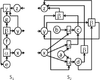
(A)

(B)

Figure 2. $S_{1}$ and $S_{2}$ are two open Petri nets. (A) Part of the infinite transition system of $\langle S_{2},a\rangle$. (B) The symbolic transition system of $\langle S_{2},a\rangle$, $\langle S_{2},b\rangle$ and $\langle S_{2},cy\rangle$.

It is worth noting that standard P/T Petri nets can be thought of as open nets whose sets $I$ and $O$ are empty. Figure 2 shows two open nets where, as usual, circles represents places and rectangles transitions (labeled with $\alpha,\beta,\chi$). Arrows from places to transitions represent $pre$, while arrows from transitions to places represent $post$. Input places are denoted by ingoing edges, while output places are denoted by outgoing edges. Thus in $S_{1}$, $x$ and $y$ are output places, while $z$ is the only input place. In $S_{2}$, it is the converse. The parallel composition of two nets is defined by attaching them on their input and output places. As an example, we can compose $S_{1}$ and $S_{2}$ by attaching them through $x,y$ and $z$.

(tr) $\frac{\displaystyle t\in T\quad\lambda(t)=l\quad m={\rm Phys.~{}Rev.~{}E}{t}\oplus c}{\displaystyle N,m\stackrel{{\scriptstyle l}}{{\mathord{\smash{-}}\mkern-6.0mu\cleaders\hbox{$\mkern-2.0mu\mathord{\smash{-}}\mkern-2.0mu$}\hfill\mkern-6.0mu\mathord{\rightarrow}}}N,{t}{{}^{\bullet}}\oplus c}$

(in) $\frac{\displaystyle i\in I_{N}}{\displaystyle N,m\stackrel{{\scriptstyle+i}}{{\mathord{\smash{-}}\mkern-6.0mu\cleaders\hbox{$\mkern-2.0mu\mathord{\smash{-}}\mkern-2.0mu$}\hfill\mkern-6.0mu\mathord{\rightarrow}}}N,m\oplus i}$

(out) $\frac{\displaystyle o\in O_{N}\quad o\in m}{\displaystyle N,m\stackrel{{\scriptstyle-o}}{{\mathord{\smash{-}}\mkern-6.0mu\cleaders\hbox{$\mkern-2.0mu\mathord{\smash{-}}\mkern-2.0mu$}\hfill\mkern-6.0mu\mathord{\rightarrow}}}N,m\ominus o}$

Table 2. Operational Semantics of marked open nets.

The operational semantics of marked open nets is expressed by the rules on Table 2, where we use ${\rm Phys.~{}Rev.~{}E}{t}$ and ${t}{{}^{\bullet}}$ to denote $pre(t)$ and $post(t)$ and we avoid putting bracket around the marked net $\langle N,m\rangle$, in order to make lighter the notation. The rule (tr) is the standard rule of P/T nets (seen as multisets rewriting), while the other two are specific of open nets. The rule (in) states that in any moment a token can be inserted inside an input place and, for this reason, the lts has always an infinite number of states. The rule (out) states that when a token is in an output place, it can be removed. Figure 2(A) shows part of the infinite transition system of $\langle S_{2},a\rangle$.

The abstract semantics is defined in [2] as the standard bisimilarity (denoted by $\sim^{N}$) and it is a congruence under the parallel composition outlined above. This is due to the rules (in) and (out), since they put a marked net in all the possible contexts. If we consider just the rule (tr), then bisimilarity fails to be a congruence. Thus also for open nets, the canonical definition of bisimulation consists in inserting the system in all the possible contexts and observing what happens.

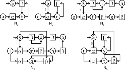
(A) (B)

(C)

Figure 3. The open nets $N_{1}$, $N_{2}$, $N_{3}$, $N_{4}$ and $N_{5}$. (A) Part of the infinite transition system of $\langle N_{1},a\rangle$. (B) Part of the infinite saturated transition system of $\langle N_{1},a\rangle$. (C) The symbolic transition systems of $\langle N_{1},a\rangle$,$\langle N_{2},c\rangle$,$\langle N_{3},e\rangle$,$\langle N_{4},l\rangle$ and $\langle N_{5},r\rangle$.

In the remainder of the paper we will use as running example the open nets in Figure 3. Since all the places have different names (with the exception of $\$$), in order to make lighter the notation, we write only the marking to mean the corresponding marked net, e.g. $b^{2}\$$ means the marked net $\langle N_{1},b^{2}\$\rangle$.

The marked net $a$ (i.e., $\langle N_{1},a\rangle$) represents a system that provides a service $\beta$. After the activation $\alpha$, it provides $\beta$ whenever the client pay one $\$$ (i.e., the environment insert a token into $\$$). The marked net $c$ instead requires five $\$$ during the activation, but then provides the service $\beta$ for free. The marked net $e$, requires three $\$$ during the activation. For three times, the service $\beta$ is performed for free and then it costs one $\$$. It is easy to see that all these marked nets are not bisimilar. Indeed, a client that has only one $\$$ can have the service $\beta$ only with $a$, while a client with five $\$$ can have the service $\beta$ for six times only with $c$. The marked net $r$ represents a system that offers the behaviour of both $a$ and $c$, i.e., either the activation $\alpha$ is for free and then the service $\beta$ costs one, or the activation costs five and then the service is for free. Also this marked net is different from all the others.

Now consider the marked net $l$. It offers the behaviour of both $a$ and $e$, but it is equivalent to $a$, i.e., $l\sim^{N}a$. Roughly, the behaviour of $e$ is absorbed by the behaviour of $a$. This is analogous to what happens in the asynchronous $\pi$-calculus where it holds that $a(x).(\overline{a}x\mid p)+\tau.p\sim^{1}\tau.p$.

The definition of $\sim^{N}$ involves an infinite transition system and thus it is often hard to check. As in the case of $\sim^{1}$ for the asynchronous $\pi$-calculus, we would like to efficiently characterize it. In the following we show an efficient characterization of $\sim^{N}$, that we have introduced in [8]. Here and in the rest of the paper, to make simpler the presentation we restrict to open nets with only input places. The general case, is completely analogous and can be found in [8, 4].

First of all, we have to define a symbolic transition system that, analogously to the operational semantics of the asynchronous $\pi$, performs input-transitions only when needed. We call it $\eta$.

Intuitively, the symbolic transition $N,m\stackrel{{\scriptstyle i,\lambda}}{{\mathord{\smash{-}}\mkern-6.0mu\cleaders\hbox{$\mkern-2.0mu\mathord{\smash{-}}\mkern-2.0mu$}\hfill\mkern-6.0mu\mathord{\rightarrow}}}_{\eta}N,m^{\prime}$ is possible if and only if $N,m\oplus i\stackrel{{\scriptstyle\lambda}}{{\mathord{\smash{-}}\mkern-6.0mu\cleaders\hbox{$\mkern-2.0mu\mathord{\smash{-}}\mkern-2.0mu$}\hfill\mkern-6.0mu\mathord{\rightarrow}}}N,m^{\prime}$ and $i$ is the smallest multiset (on input places) allowing such transition. This transition system is formally defined by the following rule.

$$\frac{\displaystyle t\in T\quad l(t)=\lambda\quad m=(m\cap{\rm Phys.~{}Rev.~{}E}{t})\oplus n\quad i\subseteq I^{\oplus}\quad{\rm Phys.~{}Rev.~{}E}{t}=(m\cap{\rm Phys.~{}Rev.~{}E}{t})\oplus i}{\displaystyle N,m\stackrel{{\scriptstyle i,\lambda}}{{\mathord{\smash{-}}\mkern-6.0mu\cleaders\hbox{$\mkern-2.0mu\mathord{\smash{-}}\mkern-2.0mu$}\hfill\mkern-6.0mu\mathord{\rightarrow}}}_{\eta}N,{t}{{}^{\bullet}}\oplus n}$$

The marking $m\cap{\rm Phys.~{}Rev.~{}E}{t}$ contains all the tokens of $m$ that are needed to perform the transition $t$. The marking $n$ contains all the tokens of $m$ that are not useful for performing $t$, while the marking $i$ contains all the tokens that $m$ needs to reach ${\rm Phys.~{}Rev.~{}E}{t}$. Note that $i$ is exactly the smallest multiset that is needed to perform the transition $t$. Indeed if we take $i_{1}$ strictly included into $i$, $m\oplus i_{1}$ cannot match ${\rm Phys.~{}Rev.~{}E}{t}$. As an example consider the net $N_{2}$ in Figure 3 with marking $cd\$^{2}$ and let $t$ be the only transition labeled with $\alpha$. We have that $cd\$^{2}\cap{\rm Phys.~{}Rev.~{}E}{t}=c\$^{2}$, $n=d$ and $i=\$^{3}$. Thus $N_{2},cd\$^{2}\stackrel{{\scriptstyle\$^{3},\alpha}}{{\mathord{\smash{-}}\mkern-6.0mu\cleaders\hbox{$\mkern-2.0mu\mathord{\smash{-}}\mkern-2.0mu$}\hfill\mkern-6.0mu\mathord{\rightarrow}}}_{\eta}N_{2},dd$, meaning that $cd\$^{2}$ needs $\$^{3}$ to perform $\alpha$ and going into $dd$. Figure 3(C) shows some symbolic transition systems.

Note that analogously to $\sim^{SYN}$ for the asynchronous $\pi$-calculus, the ordinary definition of bisimilarity on the symbolic transition systems for nets, does not coincide with $\sim^{N}$. Indeed the symbolic transition systems of $a$ and $l$ in Figure 3(C) are not bisimilar, but as discussed above, $a\sim^{N}l$. In order to efficiently characterize $\sim^{N}$, we have to introduce the following definition.

[Net-symbolic Bisimilarity] A symmetric relation $R$ is a net-symbolic bisimulation iff, whenever $\langle N_{1},m_{1}\rangle\;R\;\langle N_{2},m_{2}\rangle$:

1. if $\langle N_{1},m_{1}\rangle\stackrel{{\scriptstyle i,\lambda}}{{\mathord{\smash{-}}\mkern-6.0mu\cleaders\hbox{$\mkern-2.0mu\mathord{\smash{-}}\mkern-2.0mu$}\hfill\mkern-6.0mu\mathord{\rightarrow}}}_{\eta}\langle N_{1},m_{1}^{\prime}\rangle$, then exists a marking $m_{2}^{\prime}$ and $\exists j,k\in I^{\oplus}$ such that:

   1. $i=j\oplus k$,

   2. $\langle N_{2},m_{2}\rangle\stackrel{{\scriptstyle j,\lambda}}{{\mathord{\smash{-}}\mkern-6.0mu\cleaders\hbox{$\mkern-2.0mu\mathord{\smash{-}}\mkern-2.0mu$}\hfill\mkern-6.0mu\mathord{\rightarrow}}}_{\eta}\langle N_{2},m_{2}^{\prime}\rangle$ and

   3. $\langle N_{1},m_{1}^{\prime}\rangle\;R\;\langle N_{2},m_{2}^{\prime}\oplus k\rangle$.

Two marked nets are net-symbolic bisimilar (written $\sim^{NS}$) whenever there is a symbolic bisimulation relating them. For instance, the symmetric closure of the following relation is a net-symbolic bisimulation.

$$R=\{(l,a),\;(q,b),\;(m,b\$^{3}),\;(n,b\$^{2}),\;(o,b\$),\;(p,b)\}$$

In [8], we have shown that $\sim^{N}=\sim^{NS}$. In Section 4, we will show that the former is an instance of saturated bisimilarity, while the latter is an instance of symbolic bisimilarity. In Section 7.1 and 7.2, we will give a coalgebraic characterization of both $\sim^{N}$ and $\sim^{NS}$ by mean of saturated and normalized coalgebras.

3. A Simple Words Calculus

In the next section we will show a theoretical framework encompassing both asynchronous $\pi$-calculus and open Petri nets. In this section, we introduce a simple words calculus (swc) as a further instance of the framework presented in the next section. The aim of this “toy calculus” is to provide a more gentle example of the concepts that will be introduced afterward, by avoiding all the technicalities that arise with “real formalisms” like asynchronous $\pi$-calculus and open Petri nets.

Let $A$ be an alphabet of symbols (ranged over by $a,b,c\dots$) and $A^{*}$ be the set of finite words over $A$ (ranged over by $u,v,w\dots$). We use $\varepsilon$ to denote the empty word and $uv$ to denote the concatenation of the words $u$ and $v$. The set of processes is defined by the following grammar (where $u\in A^{*}$).

$$p::=\mathbf{0},\;\;u.p,\;\;p_{1}+p_{2}$$

A configuration is a pair $u\rhd p$ where $u$ is a word (in $A^{*}$) representing some resources and $p$ a process (generated by the above grammar). The set of all configurations (ranged over by $\gamma_{1},\gamma_{2},\dots$) is denoted by $Conf$. The algebra $\mathbb{W}$ has as carrier-set $Conf$ and as operators the words $v\in A^{*}$. The function $v_{\mathbb{W}}:Conf\to Conf$ maps each configuration $u\rhd p$ into $uv\rhd p$. Intuitively, $v_{\mathbb{W}}$ represents a context where configurations can be inserted: the effect of this insertion is that of adding $v$ (via word-concatenation) to the resources of the configuration. This is analogous to asynchronous $\pi$-calculus and open nets. There, resources are respectively outputs (in parallel) and tokens (in input places). Moreover, in those formalisms the environment can arbitrarily add new resources (via context composition).

Differently from asynchronous $\pi$ and open nets, in swc all the transitions are labeled with the same observation $\bullet$. Therefore, we fix the set of observations of swc to be $O_{\mathcal{W}}=\{\bullet\}$ (the subscript $\mathcal{W}$ will be useful later to distinguish the observations of swc from those of asynchronous $\pi$ and open nets). The operational semantics of swc is given by the transition relation $tr_{\mathcal{W}}\subseteq Conf\times O_{\mathcal{W}}\times Conf$ defined by the following rules (together with the symmetric one for $+$).

$$uv\rhd u.p\stackrel{{\scriptstyle\bullet}}{{\mathord{\smash{-}}\mkern-6.0mu\cleaders\hbox{$\mkern-2.0mu\mathord{\smash{-}}\mkern-2.0mu$}\hfill\mkern-6.0mu\mathord{\rightarrow}}}uv\rhd p\qquad\frac{\displaystyle u\rhd p\stackrel{{\scriptstyle\bullet}}{{\mathord{\smash{-}}\mkern-6.0mu\cleaders\hbox{$\mkern-2.0mu\mathord{\smash{-}}\mkern-2.0mu$}\hfill\mkern-6.0mu\mathord{\rightarrow}}}u\rhd p^{\prime}}{\displaystyle u\rhd p+q\stackrel{{\scriptstyle\bullet}}{{\mathord{\smash{-}}\mkern-6.0mu\cleaders\hbox{$\mkern-2.0mu\mathord{\smash{-}}\mkern-2.0mu$}\hfill\mkern-6.0mu\mathord{\rightarrow}}}u\rhd p^{\prime}}$$

Intuitively, the process $u.p$ needs the resources $u$ in order to evolve. If $u$ is present in the configuration (as a suffix) then, $u.p$ becomes $p$. Note that, differently from asynchronous $\pi$ and open nets, the resources $u$ are not consumed, but only “read” (we have chosen to give this read-behavior to swc, just for simplifying the following examples).

[Saturated Bisimilarity for swc] Let $R\subseteq Conf\times Conf$ be a symmetric relation. $R$ is a saturated bisimulation iff, $\forall v\in A^{*}$, whenever $\gamma_{1}\;R\;\gamma_{2}$:

1. $v_{\mathbb{W}}(\gamma_{1})\,R\,v_{\mathbb{W}}(\gamma_{2})$,

2. if $\gamma_{1}\stackrel{{\scriptstyle\bullet}}{{\mathord{\smash{-}}\mkern-6.0mu\cleaders\hbox{$\mkern-2.0mu\mathord{\smash{-}}\mkern-2.0mu$}\hfill\mkern-6.0mu\mathord{\rightarrow}}}\gamma_{1}^{\prime}$, then $\exists\gamma_{2}^{\prime}$ such that $\gamma_{2}\stackrel{{\scriptstyle\bullet}}{{\mathord{\smash{-}}\mkern-6.0mu\cleaders\hbox{$\mkern-2.0mu\mathord{\smash{-}}\mkern-2.0mu$}\hfill\mkern-6.0mu\mathord{\rightarrow}}}\gamma_{2}^{\prime}$ and $\gamma_{1}^{\prime}\;R\;\gamma_{2}^{\prime}$.

We write $\gamma_{1}\sim^{S}\gamma_{2}$ iff there is a saturated bisimulation $R$ such that $\gamma_{1}\;R\;\gamma_{2}$.

For instance, the configurations $ab\rhd ab.\mathbf{0}$ and $ab\rhd\varepsilon.\mathbf{0}$ are saturated bisimilar, because for any word $v$ both $abv\rhd ab.\mathbf{0}$ and $abv\rhd\varepsilon.\mathbf{0}$ can only perform one transition and then stop. A more interesting example is the following. For all words $u,v\in A^{*}$ such that $v=uw$ (i.e., $u$ is a prefix of $v$), it holds that

$$\varepsilon\rhd u.p+v.p\sim^{S}\varepsilon\rhd u.p$$

because for any word $v^{\prime}\in A^{*}$, $v^{\prime}\rhd u.p+v.p$ and $v^{\prime}\rhd u.p$ have the same behaviour. For those $v^{\prime}$ having $u$ as prefix (i.e., $v^{\prime}=uw^{\prime}$), both the configurations can only perform transitions going into $v^{\prime}\rhd p$; for those $v^{\prime}$ where $u$ is not a prefix, both the configurations stop. As it happens for the asynchronous $\pi$-calculus and open nets, the behaviour of $v.p$ is somehow “absorbed” by the behaviour of $u.p$. By joining the two previous examples, we have that:

$$\varepsilon\rhd a.ab.\mathbf{0}+ab.\varepsilon.\mathbf{0}\sim^{S}\varepsilon\rhd a.ab.\mathbf{0}$$

Indeed, for all the words $v^{\prime}\in A^{*}$ having $ab$ as a prefix (i.e., $v^{\prime}=abw^{\prime}$) the configuration $abw^{\prime}\rhd a.ab.\mathbf{0}+ab.\varepsilon.\mathbf{0}$ can go either in $abw^{\prime}\rhd ab.\mathbf{0}$ or in $abw^{\prime}\rhd\varepsilon.\mathbf{0}$, while the configuration $abw^{\prime}\rhd a.ab.\mathbf{0}$ can only go in $abw^{\prime}\rhd ab.\mathbf{0}$ that, as shown in our first example, is bisimilar to $abw^{\prime}\rhd\varepsilon.\mathbf{0}$. For all the other words, the two configuration behave exactly in the same way.

For simplifying the explanation, it is useful to introduce the saturated transition system: $u\rhd p\stackrel{{\scriptstyle v,\bullet}}{{\mathord{\smash{-}}\mkern-6.0mu\cleaders\hbox{$\mkern-2.0mu\mathord{\smash{-}}\mkern-2.0mu$}\hfill\mkern-6.0mu\mathord{\rightarrow}}}_{S}u^{\prime}\rhd p^{\prime}$ iff $uv\rhd p\stackrel{{\scriptstyle\bullet}}{{\mathord{\smash{-}}\mkern-6.0mu\cleaders\hbox{$\mkern-2.0mu\mathord{\smash{-}}\mkern-2.0mu$}\hfill\mkern-6.0mu\mathord{\rightarrow}}}u^{\prime}\rhd p^{\prime}$. It is easy to see that the standard notion of bisimilarity on this transition system coincides with $\sim^{S}$. The saturated transition systems of $\varepsilon\rhd u.p+v.p$ and $\varepsilon\rhd u.p$ are shown in Figure 4(A). For making lighter the notation, in that figure and in the following ones we have omitted the observation $\bullet$. Note that $\varepsilon\rhd u.p+v.p$ and $\varepsilon\rhd u.p$ perform the same saturated transitions (and thus they are saturated bisimilar, as discussed above).

Figure 4. (A) The saturated transition systems of $\varepsilon\rhd u.p+v.p$ and $\varepsilon\rhd u.p$. (B) The symbolic transition systems of $\varepsilon\rhd u.p+v.p$ and $\varepsilon\rhd u.p$. (C) The symbolic transition systems of $\gamma_{1}=\varepsilon\rhd a.ab.\mathbf{0}+ab.\varepsilon.\mathbf{0}$ and $\gamma_{2}=\varepsilon\rhd a.ab.\mathbf{0}$.

In order to give a more efficient characterization of $\sim^{S}$ (that avoids the quantification over all words $v\in A^{*}$), we define a symbolic transition system that, like the saturated transition system, is labeled with pairs $v,\bullet$ (for $v\in A^{*}$). The main difference is that a symbolic transition $u\rhd p\stackrel{{\scriptstyle v,\bullet}}{{\mathord{\smash{-}}\mkern-6.0mu\cleaders\hbox{$\mkern-2.0mu\mathord{\smash{-}}\mkern-2.0mu$}\hfill\mkern-6.0mu\mathord{\rightarrow}}}_{\omega}u^{\prime}\rhd p^{\prime}$ is performed only when $v$ is the “minimal word” such that $uv\rhd p\stackrel{{\scriptstyle\bullet}}{{\mathord{\smash{-}}\mkern-6.0mu\cleaders\hbox{$\mkern-2.0mu\mathord{\smash{-}}\mkern-2.0mu$}\hfill\mkern-6.0mu\mathord{\rightarrow}}}u^{\prime}\rhd p^{\prime}$. The symbolic transition system $\omega\subseteq Conf\times A^{*}\times O_{\mathcal{W}}\times Conf$ is defined by the following rules (together with the symmetric rule for $+$).

$$uv\rhd u.p\stackrel{{\scriptstyle\varepsilon,\bullet}}{{\mathord{\smash{-}}\mkern-6.0mu\cleaders\hbox{$\mkern-2.0mu\mathord{\smash{-}}\mkern-2.0mu$}\hfill\mkern-6.0mu\mathord{\rightarrow}}}_{\omega}uv\rhd p\qquad u\rhd uv.p\stackrel{{\scriptstyle v,\bullet}}{{\mathord{\smash{-}}\mkern-6.0mu\cleaders\hbox{$\mkern-2.0mu\mathord{\smash{-}}\mkern-2.0mu$}\hfill\mkern-6.0mu\mathord{\rightarrow}}}_{\omega}uv\rhd p\qquad\frac{\displaystyle u\rhd p\stackrel{{\scriptstyle v,\bullet}}{{\mathord{\smash{-}}\mkern-6.0mu\cleaders\hbox{$\mkern-2.0mu\mathord{\smash{-}}\mkern-2.0mu$}\hfill\mkern-6.0mu\mathord{\rightarrow}}}_{\omega}u^{\prime}\rhd p^{\prime}}{\displaystyle u\rhd p+q\stackrel{{\scriptstyle v,\bullet}}{{\mathord{\smash{-}}\mkern-6.0mu\cleaders\hbox{$\mkern-2.0mu\mathord{\smash{-}}\mkern-2.0mu$}\hfill\mkern-6.0mu\mathord{\rightarrow}}}_{\omega}u^{\prime}\rhd p^{\prime}}$$

In the central rule, the process $uv.p$ needs the resources $uv$ to evolve. In the configuration, there are only $u$ resources and thus the process “takes from the environment” the word $v$. In the leftmost rule, all the needed resources ($u$) are already present in the configuration (as a prefix) and thus the process can evolve without taking resources from the environment (i.e., by taking $\varepsilon$). The symbolic transition systems of $\varepsilon\rhd u.p+v.p$ and $\varepsilon\rhd u.p$ are depicted in Figure 4(B). Note that the former process can perform one symbolic transition more than the latter, even if they perform the same saturated transitions. The symbolic transition systems of $\gamma_{1}=\varepsilon\rhd a.ab.\mathbf{0}+ab.\varepsilon.\mathbf{0}$ and $\gamma_{2}=\varepsilon\rhd a.ab.\mathbf{0}$ are shown in Figure 4(C).

Note that the standard notion of bisimilarity defined over $\stackrel{{\scriptstyle v,\bullet}}{{\mathord{\smash{-}}\mkern-6.0mu\cleaders\hbox{$\mkern-2.0mu\mathord{\smash{-}}\mkern-2.0mu$}\hfill\mkern-6.0mu\mathord{\rightarrow}}}_{\omega}$ (hereafter called syntactic bisimilarity and denoted by $\sim^{W}$) is strictly included into $\sim^{S}$. For example, $\varepsilon\rhd u.p$ and $\varepsilon\rhd u.p+v.p$ (with $u$ prefix of $v$) are in $\sim^{S}$ but not in $\sim^{W}$ because $\varepsilon\rhd u.p+v.p\stackrel{{\scriptstyle v,\bullet}}{{\mathord{\smash{-}}\mkern-6.0mu\cleaders\hbox{$\mkern-2.0mu\mathord{\smash{-}}\mkern-2.0mu$}\hfill\mkern-6.0mu\mathord{\rightarrow}}}_{\omega}v\rhd p$, while $\varepsilon\rhd u.p$ only performs a symbolic transition labeled with $u$. The same holds for $\varepsilon\rhd a.ab.\mathbf{0}+ab.\varepsilon.\mathbf{0}$ and $\varepsilon\rhd a.ab.\mathbf{0}$.

In order to capture $\sim^{S}$ by exploiting the symbolic transition system we need a more elaborated notion of bisimulation that relies on an inference system. For better explaining it, observe that the following “monotonicity property” holds:

$\forall v\in A^{*}$ and $\forall u\rhd p,u^{\prime}\rhd p^{\prime}\in Conf$, if $u\rhd p\stackrel{{\scriptstyle\bullet}}{{\mathord{\smash{-}}\mkern-6.0mu\cleaders\hbox{$\mkern-2.0mu\mathord{\smash{-}}\mkern-2.0mu$}\hfill\mkern-6.0mu\mathord{\rightarrow}}}u^{\prime}\rhd p^{\prime}$, then $uv\rhd p\stackrel{{\scriptstyle\bullet}}{{\mathord{\smash{-}}\mkern-6.0mu\cleaders\hbox{$\mkern-2.0mu\mathord{\smash{-}}\mkern-2.0mu$}\hfill\mkern-6.0mu\mathord{\rightarrow}}}u^{\prime}v\rhd p^{\prime}$.

This property states that when adding the resources $v$ to the original configuration (or, equivalently, when inserting the configuration into the context $v_{\mathbb{W}}(-)$), all the transitions of the original configuration are preserved. This is analogous to what happens in the asynchronous $\pi$-calculus (where putting outputs in parallel does not inhibit any transition) and in open Petri nets (where inserting tokens in input places does not inhibit any transition).

An inference system is a set of rules stating properties like those just described. For the case of swc, the inference system $T_{\mathcal{W}}$ is defined by the following rule (parametric w.r.t. $v\in A^{*}$).

$$\frac{\displaystyle\gamma\stackrel{{\scriptstyle\bullet}}{{\mathord{\smash{-}}\mkern-6.0mu\cleaders\hbox{$\mkern-2.0mu\mathord{\smash{-}}\mkern-2.0mu$}\hfill\mkern-6.0mu\mathord{\rightarrow}}}\gamma^{\prime}}{\displaystyle v_{\mathbb{W}}(\gamma)\stackrel{{\scriptstyle\bullet}}{{\mathord{\smash{-}}\mkern-6.0mu\cleaders\hbox{$\mkern-2.0mu\mathord{\smash{-}}\mkern-2.0mu$}\hfill\mkern-6.0mu\mathord{\rightarrow}}}v_{\mathbb{W}}(\gamma^{\prime})}$$

This rule just states the above monotonicity property. Moreover, it induces a derivation relation $\vdash_{T_{\mathcal{W}}}\subseteq(Conf\times A^{*}\times O_{\mathcal{W}}\times Conf)\times(Conf\times A^{*}\times O_{\mathcal{W}}\times Conf)$ as follows:

$$\gamma\stackrel{{\scriptstyle v,\bullet}}{{\mathord{\smash{-}}\mkern-6.0mu\cleaders\hbox{$\mkern-2.0mu\mathord{\smash{-}}\mkern-2.0mu$}\hfill\mkern-6.0mu\mathord{\rightarrow}}}\gamma^{\prime}\vdash_{T_{\mathcal{W}}}\gamma\stackrel{{\scriptstyle vw,\bullet}}{{\mathord{\smash{-}}\mkern-6.0mu\cleaders\hbox{$\mkern-2.0mu\mathord{\smash{-}}\mkern-2.0mu$}\hfill\mkern-6.0mu\mathord{\rightarrow}}}w_{\mathbb{W}}(\gamma^{\prime})$$

Consider the saturated transitions of $\varepsilon\rhd u.p+v.p$ in Figure 4(A) and fix $\gamma=\varepsilon\rhd u.p+v.p$. We have that $(\gamma\stackrel{{\scriptstyle u,\bullet}}{{\mathord{\smash{-}}\mkern-6.0mu\cleaders\hbox{$\mkern-2.0mu\mathord{\smash{-}}\mkern-2.0mu$}\hfill\mkern-6.0mu\mathord{\rightarrow}}}_{S}u\rhd p)\vdash_{T_{\mathcal{W}}}(\gamma\stackrel{{\scriptstyle ua,\bullet}}{{\mathord{\smash{-}}\mkern-6.0mu\cleaders\hbox{$\mkern-2.0mu\mathord{\smash{-}}\mkern-2.0mu$}\hfill\mkern-6.0mu\mathord{\rightarrow}}}_{S}ua\rhd p)\vdash_{T_{\mathcal{W}}}(\gamma\stackrel{{\scriptstyle uaa,\bullet}}{{\mathord{\smash{-}}\mkern-6.0mu\cleaders\hbox{$\mkern-2.0mu\mathord{\smash{-}}\mkern-2.0mu$}\hfill\mkern-6.0mu\mathord{\rightarrow}}}_{S}uaa\rhd p)\vdash_{T_{\mathcal{W}}}\dots$ More generally, $\forall w\in A^{*}$,

$$\gamma\stackrel{{\scriptstyle u,\bullet}}{{\mathord{\smash{-}}\mkern-6.0mu\cleaders\hbox{$\mkern-2.0mu\mathord{\smash{-}}\mkern-2.0mu$}\hfill\mkern-6.0mu\mathord{\rightarrow}}}_{S}u\rhd p\vdash_{T_{\mathcal{W}}}\gamma\stackrel{{\scriptstyle uw,\bullet}}{{\mathord{\smash{-}}\mkern-6.0mu\cleaders\hbox{$\mkern-2.0mu\mathord{\smash{-}}\mkern-2.0mu$}\hfill\mkern-6.0mu\mathord{\rightarrow}}}_{S}uw\rhd p$$

and in the case of $\gamma=\varepsilon\rhd u.p+v.p$ in Figure 4(B), this means that

$$\gamma\stackrel{{\scriptstyle u,\bullet}}{{\mathord{\smash{-}}\mkern-6.0mu\cleaders\hbox{$\mkern-2.0mu\mathord{\smash{-}}\mkern-2.0mu$}\hfill\mkern-6.0mu\mathord{\rightarrow}}}_{\omega}u\rhd p\vdash_{T_{\mathcal{W}}}\gamma\stackrel{{\scriptstyle v,\bullet}}{{\mathord{\smash{-}}\mkern-6.0mu\cleaders\hbox{$\mkern-2.0mu\mathord{\smash{-}}\mkern-2.0mu$}\hfill\mkern-6.0mu\mathord{\rightarrow}}}_{\omega}v\rhd p\text{.}$$

This is somehow useful to understand the causes of the mismatch between $\sim^{S}$ and $\sim^{W}$ (syntactic bisimilarity). First, observe that symbolic transitions can derive through $T_{\mathcal{W}}$ all and only the saturated transitions (this will be formally shown in the next section). Then, recall that the configurations $\varepsilon\rhd u.p+v.p$ and $\varepsilon\rhd u.p$ are in $\sim^{S}$ because can perform the same saturated transitions, but they are not in $\sim^{W}$ because the former can perform the symbolic transition $\stackrel{{\scriptstyle v,\bullet}}{{\mathord{\smash{-}}\mkern-6.0mu\cleaders\hbox{$\mkern-2.0mu\mathord{\smash{-}}\mkern-2.0mu$}\hfill\mkern-6.0mu\mathord{\rightarrow}}}_{\omega}$. This symbolic transition is redundant since it can be derived from $\stackrel{{\scriptstyle u,\bullet}}{{\mathord{\smash{-}}\mkern-6.0mu\cleaders\hbox{$\mkern-2.0mu\mathord{\smash{-}}\mkern-2.0mu$}\hfill\mkern-6.0mu\mathord{\rightarrow}}}_{\omega}$ through the inference system $T_{\mathcal{W}}$. More explicitly, all the saturated transitions that can be derived from $\stackrel{{\scriptstyle v,\bullet}}{{\mathord{\smash{-}}\mkern-6.0mu\cleaders\hbox{$\mkern-2.0mu\mathord{\smash{-}}\mkern-2.0mu$}\hfill\mkern-6.0mu\mathord{\rightarrow}}}_{\omega}$ can also be derived from $\stackrel{{\scriptstyle u,\bullet}}{{\mathord{\smash{-}}\mkern-6.0mu\cleaders\hbox{$\mkern-2.0mu\mathord{\smash{-}}\mkern-2.0mu$}\hfill\mkern-6.0mu\mathord{\rightarrow}}}_{\omega}$ and thus $\stackrel{{\scriptstyle v,\bullet}}{{\mathord{\smash{-}}\mkern-6.0mu\cleaders\hbox{$\mkern-2.0mu\mathord{\smash{-}}\mkern-2.0mu$}\hfill\mkern-6.0mu\mathord{\rightarrow}}}_{\omega}$ does not add any meaningful information about the saturated behaviour of the configuration. We can avoid this problem by employing the following notion of bisimulation.

[Symbolic Bisimilarity for swc] Let $R\subseteq Conf\times Conf$ be a symmetric relation. $R$ is a symbolic bisimulation iff whenever $\gamma_{1}\;R\;\gamma_{2}$:

1. if $\gamma_{1}\stackrel{{\scriptstyle v,\bullet}}{{\mathord{\smash{-}}\mkern-6.0mu\cleaders\hbox{$\mkern-2.0mu\mathord{\smash{-}}\mkern-2.0mu$}\hfill\mkern-6.0mu\mathord{\rightarrow}}}_{\omega}\gamma_{1}^{\prime}$, then $\exists\gamma_{2}^{\prime},\gamma_{2}^{\prime\prime}\in Conf,u\in A^{*}$ s.t. $\gamma_{2}\stackrel{{\scriptstyle u,\bullet}}{{\mathord{\smash{-}}\mkern-6.0mu\cleaders\hbox{$\mkern-2.0mu\mathord{\smash{-}}\mkern-2.0mu$}\hfill\mkern-6.0mu\mathord{\rightarrow}}}_{\omega}\gamma_{2}^{\prime}$, $\gamma_{2}\stackrel{{\scriptstyle u,\bullet}}{{\mathord{\smash{-}}\mkern-6.0mu\cleaders\hbox{$\mkern-2.0mu\mathord{\smash{-}}\mkern-2.0mu$}\hfill\mkern-6.0mu\mathord{\rightarrow}}}_{\omega}\gamma_{2}^{\prime}\vdash_{T_{\mathcal{W}}}\gamma_{2}\stackrel{{\scriptstyle v,\bullet}}{{\mathord{\smash{-}}\mkern-6.0mu\cleaders\hbox{$\mkern-2.0mu\mathord{\smash{-}}\mkern-2.0mu$}\hfill\mkern-6.0mu\mathord{\rightarrow}}}\gamma_{2}^{\prime\prime}$ and $\gamma_{1}^{\prime}\;R\;\gamma_{2}^{\prime\prime}$.

We write $\gamma_{1}\sim^{SYM}\gamma_{2}$ iff there is a symbolic bisimulation $R$ such that $\gamma_{1}\;R\;\gamma_{2}$.

For example $\varepsilon\rhd u.p+v.p\sim^{SYM}\varepsilon\rhd u.p$ (when $v=uw$), because if $\varepsilon\rhd u.p+v.p\stackrel{{\scriptstyle v,\bullet}}{{\mathord{\smash{-}}\mkern-6.0mu\cleaders\hbox{$\mkern-2.0mu\mathord{\smash{-}}\mkern-2.0mu$}\hfill\mkern-6.0mu\mathord{\rightarrow}}}_{\omega}v\rhd p$, then $\varepsilon\rhd u.p\stackrel{{\scriptstyle u,\bullet}}{{\mathord{\smash{-}}\mkern-6.0mu\cleaders\hbox{$\mkern-2.0mu\mathord{\smash{-}}\mkern-2.0mu$}\hfill\mkern-6.0mu\mathord{\rightarrow}}}_{\omega}u\rhd p$ and this transition derives $\varepsilon\rhd u.p\stackrel{{\scriptstyle uw,\bullet}}{{\mathord{\smash{-}}\mkern-6.0mu\cleaders\hbox{$\mkern-2.0mu\mathord{\smash{-}}\mkern-2.0mu$}\hfill\mkern-6.0mu\mathord{\rightarrow}}}_{\omega}w_{\mathbb{W}}(u\rhd p)$ that is $\varepsilon\rhd u.p\stackrel{{\scriptstyle v,\bullet}}{{\mathord{\smash{-}}\mkern-6.0mu\cleaders\hbox{$\mkern-2.0mu\mathord{\smash{-}}\mkern-2.0mu$}\hfill\mkern-6.0mu\mathord{\rightarrow}}}_{\omega}v\rhd p$.

For an example of symbolic bisimulation, take $\gamma_{1}=\varepsilon\rhd a.ab.\mathbf{0}+ab.\varepsilon.\mathbf{0}$ and $\gamma_{2}=\varepsilon\rhd a.ab.\mathbf{0}$ in Figure 4(C) and consider the symmetric closure of the following relation.

$$R=\{(\gamma_{1},\gamma_{2}),\;(a\rhd ab.\mathbf{0},a\rhd ab.\mathbf{0}),\;(ab\rhd\varepsilon.\mathbf{0},ab\rhd ab.\mathbf{0}),\;(ab\rhd\mathbf{0},ab\rhd\mathbf{0})\}$$

For the last three pairs, it is easy to check that the configurations satisfy the above requirements. For $(\gamma_{1},\gamma_{2})$, this is more interesting: the transition $\gamma_{1}\stackrel{{\scriptstyle ab,\bullet}}{{\mathord{\smash{-}}\mkern-6.0mu\cleaders\hbox{$\mkern-2.0mu\mathord{\smash{-}}\mkern-2.0mu$}\hfill\mkern-6.0mu\mathord{\rightarrow}}}_{\omega}ab\rhd\varepsilon.\mathbf{0}$ can be matched by $\gamma_{2}\stackrel{{\scriptstyle a,\bullet}}{{\mathord{\smash{-}}\mkern-6.0mu\cleaders\hbox{$\mkern-2.0mu\mathord{\smash{-}}\mkern-2.0mu$}\hfill\mkern-6.0mu\mathord{\rightarrow}}}_{\omega}a\rhd ab.\mathbf{0}$ because, by definition of $\vdash_{T_{\mathcal{W}}}$, $\gamma_{2}\stackrel{{\scriptstyle a,\bullet}}{{\mathord{\smash{-}}\mkern-6.0mu\cleaders\hbox{$\mkern-2.0mu\mathord{\smash{-}}\mkern-2.0mu$}\hfill\mkern-6.0mu\mathord{\rightarrow}}}_{\omega}a\rhd ab.\mathbf{0}\vdash_{T_{\mathcal{W}}}\gamma_{2}\stackrel{{\scriptstyle ab,\bullet}}{{\mathord{\smash{-}}\mkern-6.0mu\cleaders\hbox{$\mkern-2.0mu\mathord{\smash{-}}\mkern-2.0mu$}\hfill\mkern-6.0mu\mathord{\rightarrow}}}ab\rhd ab.\mathbf{0}$ and $(ab\rhd\varepsilon.\mathbf{0},ab\rhd ab.\mathbf{0})\in R$.

In the next section we will show that $\sim^{S}=\sim^{SYM}$. Before concluding this section, it is worth to make a final remark. The reader would have thought that in order to retrieve $\sim^{S}$ from the symbolic transition system, one could just remove all the “redundant transitions”, i.e., all those symbolic transitions $\gamma\stackrel{{\scriptstyle v,\bullet}}{{\mathord{\smash{-}}\mkern-6.0mu\cleaders\hbox{$\mkern-2.0mu\mathord{\smash{-}}\mkern-2.0mu$}\hfill\mkern-6.0mu\mathord{\rightarrow}}}_{\omega}\gamma^{\prime\prime}$ such that there exists another symbolic transition $\gamma\stackrel{{\scriptstyle u,\bullet}}{{\mathord{\smash{-}}\mkern-6.0mu\cleaders\hbox{$\mkern-2.0mu\mathord{\smash{-}}\mkern-2.0mu$}\hfill\mkern-6.0mu\mathord{\rightarrow}}}_{\omega}\gamma^{\prime}$ deriving it (in Section 7 this removal will be called normalization). It is important to show that this is not enough to retrieve $\sim^{S}$: consider the symbolic transition systems of $\gamma_{1}=\varepsilon\rhd a.ab.\mathbf{0}+ab.\varepsilon.\mathbf{0}$ and $\gamma_{2}=\varepsilon\rhd a.ab.\mathbf{0}$ shown in Figure 4(C). They have no redundant transitions, but still $\gamma_{1}\sim^{S}\gamma_{2}$ and $\gamma_{1}\not\sim^{W}\gamma_{2}$. The transition $\gamma_{1}\stackrel{{\scriptstyle ab,\bullet}}{{\mathord{\smash{-}}\mkern-6.0mu\cleaders\hbox{$\mkern-2.0mu\mathord{\smash{-}}\mkern-2.0mu$}\hfill\mkern-6.0mu\mathord{\rightarrow}}}_{\omega}ab\rhd\varepsilon.\mathbf{0}$ is not redundant, because $\gamma_{1}\stackrel{{\scriptstyle a,\bullet}}{{\mathord{\smash{-}}\mkern-6.0mu\cleaders\hbox{$\mkern-2.0mu\mathord{\smash{-}}\mkern-2.0mu$}\hfill\mkern-6.0mu\mathord{\rightarrow}}}_{\omega}a\rhd ab.\mathbf{0}\not\vdash_{T_{\mathcal{W}}}\gamma_{1}\stackrel{{\scriptstyle ab,\bullet}}{{\mathord{\smash{-}}\mkern-6.0mu\cleaders\hbox{$\mkern-2.0mu\mathord{\smash{-}}\mkern-2.0mu$}\hfill\mkern-6.0mu\mathord{\rightarrow}}}_{\omega}ab\rhd\varepsilon.\mathbf{0}$, since $b_{\mathbb{W}}(a\rhd ab.\mathbf{0})=ab\rhd ab.\mathbf{0}\neq ab\rhd\varepsilon.\mathbf{0}$. However, it is semantically redundant, because $\gamma_{1}\stackrel{{\scriptstyle a,\bullet}}{{\mathord{\smash{-}}\mkern-6.0mu\cleaders\hbox{$\mkern-2.0mu\mathord{\smash{-}}\mkern-2.0mu$}\hfill\mkern-6.0mu\mathord{\rightarrow}}}_{\omega}a\rhd ab.\mathbf{0}\vdash_{T_{\mathcal{W}}}\gamma_{1}\stackrel{{\scriptstyle ab,\bullet}}{{\mathord{\smash{-}}\mkern-6.0mu\cleaders\hbox{$\mkern-2.0mu\mathord{\smash{-}}\mkern-2.0mu$}\hfill\mkern-6.0mu\mathord{\rightarrow}}}_{\omega}ab\rhd ab.\mathbf{0}$ and the states $ab\rhd ab.\mathbf{0}$ and $ab\rhd\varepsilon.\mathbf{0}$ are semantically equivalent (i.e., $ab\rhd ab.\mathbf{0}\sim^{S}ab\rhd\varepsilon.\mathbf{0}$).

In order to characterize $\sim^{S}$ through $\omega$, we should eliminate all the semantically redundant transitions, but this is impossible without knowing a priori $\sim^{S}$. This is the main motivation for the introduction of normalized coalgebras in Section 7.

4. Saturated and Symbolic Semantics

In Section 1 and Section 2, we have introduced asynchronous $\pi$-calculus and open Petri nets. In both cases, their abstract semantics is defined in two different ways: either by inserting the systems into all possible contexts (like $\sim^{1}$ and $\sim^{N}$) or by inserting the system only in those contexts that are really needed (like $\sim^{a}$ and $\sim^{NS}$). Moreover, the latter coincides with the former and thus can be thought as an efficient characterization of the former.

This sort of “double definition” of the abstract semantics recurs in many formalisms modeling interactive systems, such as mobile ambients [12], open $\pi$-calculus [41] and explicit fusion calculus [43]. In [8], we have introduced a theoretical framework that generalizes this “double definition” and encompasses all the above mentioned formalisms. In this section we recall this framework by employing as running examples the simple words calculus, the asynchronous $\pi$-calculus and open Petri nets.

4.1. Saturated Semantics

Given a small category ${\bf C}$, a $\Gamma({\bf C})$-algebra is an algebra for the algebraic specification in Figure 5 where $|{\bf C}|$ denotes the set of objects of ${\bf C}$, $||{\bf C}||$ the set of arrows of ${\bf C}$ and, for all $i,j\in|{\bf C}|$, ${\bf C}[i,j]$ denotes the set of arrows from $i$ to $j$. Thus, a $\Gamma({\bf C})$-algebra $\mathbb{X}$ consists of a $|{\bf C}|$-sorted family $X=\{X_{i}\mid i\in|{\bf C}|\}$ of sets and a function $c_{\mathbb{X}}:X_{i}\to X_{j}$ for all $c\in{\bf C}[i,j]$. Moreover, these functions must satisfy the equations in Figure 5: $id_{i_{\mathbb{X}}}$ is the identity function on $X_{i}$ and if $d;e=c$ in ${\bf C}$, $(d;e)_{\mathbb{X}}$ is equal to $c_{\mathbb{X}}$. Hereafter, we will use $\int X$ to denote the set of the elements of a $\Gamma({\bf C})$-algebra $\mathbb{X}$, namely, the disjoint union $\sum_{i\in|{\bf C}|}X_{i}$.

The main definition of the framework presented in [8] is that of context interactive systems. In our theory, an interactive system is a state-machine that can interact with the environment (contexts) through an evolving interface. [Context Interactive System] A context interactive system $\mathcal{I}$ is a quadruple $\langle{\bf C},\mathbb{X},O,tr\rangle$ where:

1. ${\bf C}$ is a small category,

2. $\mathbb{X}$ is a $\Gamma({\bf C})$-algebra,

3. $O$ is a set of observations,

4. $tr\subseteq\int X\times O\times\int X$ is a labeled transition relation ($p\stackrel{{\scriptstyle o}}{{\mathord{\smash{-}}\mkern-6.0mu\cleaders\hbox{$\mkern-2.0mu\mathord{\smash{-}}\mkern-2.0mu$}\hfill\mkern-6.0mu\mathord{\rightarrow}}}p^{\prime}$ means $(p,o,p^{\prime})\in tr$).

Intuitively, objects of ${\bf C}$ are interfaces of the system, while arrows are contexts. Every element $p$ of $X_{i}$ represents a state with interface $i$ and it can be inserted into the context $c\in{\bf C}[i,j]$, obtaining a new state $c_{\mathbb{X}}(p)$ that has interface $j$. Every state can evolve into a new state (possibly with different interface) producing an observation $o\in O$.

The abstract semantics of interactive systems is usually defined through behavioural equivalences. In [8] we proposed a general notion of bisimilarity that generalizes the abstract semantics of a large variety of formalisms [12, 1, 41, 37, 44, 11]. The idea is that two states of a system are equivalent if they are indistinguishable from an external observer that, in any moment of their execution, can insert them into some environment and then observe some transitions.

[Saturated Bisimilarity] Let $\mathcal{I}=\langle{\bf C},\mathbb{X},O,tr\rangle$ be a context interactive system. Let $R=\{R_{i}\subseteq X_{i}\times X_{i}\mid i\in|{\bf C}|\}$ be a $|{\bf C}|$-sorted family of symmetric relations. $R$ is a saturated bisimulation iff, $\forall i,j\in|{\bf C}|$, $\forall c\in{\bf C}[i,j]$, whenever $pR_{i}q$:

1. $c_{\mathbb{X}}(p)\,R_{j}\,c_{\mathbb{X}}(q)$,

2. if $p\stackrel{{\scriptstyle o}}{{\mathord{\smash{-}}\mkern-6.0mu\cleaders\hbox{$\mkern-2.0mu\mathord{\smash{-}}\mkern-2.0mu$}\hfill\mkern-6.0mu\mathord{\rightarrow}}}p^{\prime}$ with $p^{\prime}\in X_{k}$ for some $k\in|{\bf C}|$, then $\exists q^{\prime}\in X_{k}$ such that $q\stackrel{{\scriptstyle o}}{{\mathord{\smash{-}}\mkern-6.0mu\cleaders\hbox{$\mkern-2.0mu\mathord{\smash{-}}\mkern-2.0mu$}\hfill\mkern-6.0mu\mathord{\rightarrow}}}q^{\prime}$ and $p^{\prime}R_{k}q^{\prime}$.

We write $p\sim^{S}_{i}q$ iff there is a saturated bisimulation $R$ such that $pR_{i}q$. An alternative but equivalent definition can be given by defining the saturated transition system $(\textsc{satts})$ as follows: $p\stackrel{{\scriptstyle c,o}}{{\mathord{\smash{-}}\mkern-6.0mu\cleaders\hbox{$\mkern-2.0mu\mathord{\smash{-}}\mkern-2.0mu$}\hfill\mkern-6.0mu\mathord{\rightarrow}}}_{S}q$ if and only if $c_{\mathbb{X}}(p)\stackrel{{\scriptstyle o}}{{\mathord{\smash{-}}\mkern-6.0mu\cleaders\hbox{$\mkern-2.0mu\mathord{\smash{-}}\mkern-2.0mu$}\hfill\mkern-6.0mu\mathord{\rightarrow}}}q$. Trivially the ordinary bisimilarity over satts coincides with $\sim^{S}$.

Proposition 1.

$\sim^{S}$ is the coarsest bisimulation congruence.

specification $\Gamma({\bf C})$ =
	sorts
		$i$	$\forall i\in|{\bf C}|$
	operations
		$c:i\to j$	$\forall c\in{\bf C}[i,j]$
	equations
		$id_{i}(x)=x$
		$e(d(x))=c(x)$	$\forall d;e=c$

Figure 5. Algebraic specification $\Gamma({\bf C})$.

A Context Interactive Systems for swc.

In Section 3, we have introduced a simple words calculus. Here we show its context interactive system $\mathcal{W}=\langle{\bf Wor},\mathbb{W},O_{\mathcal{W}},tr_{\mathcal{W}}\rangle$. Recall that $\varepsilon$ is the empty word and that $uv$ denote the concatenation of the words $u$ and $v$. The category ${\bf Wor}$ is defined as follows:

1. $|{\bf Wor}|=\{\circ\}$;

2. ${\bf Wor}[\circ,\circ]=A^{*}$;

3. $id_{\circ}=\varepsilon$;

4. $\forall u,v\in A^{*}$, $u;v=uv$.

The algebra $\mathbb{W}$, the set of observations $O_{\mathcal{W}}$ and the transition relation $tr_{\mathcal{W}}$ have been already introduced in Section 3. In swc, all the configurations have the same interface (sort) and thus, in the category ${\bf Wor}$ there is only one object. It is easy to see that saturated bisimilarity for swc (Definition 3) is an instance of Definition 4.1.

A Context Interactive Systems for open Petri nets.

In the following we formally define $\mathcal{N}=\langle{\bf Tok},\mathbb{N},\Lambda,tr_{\mathcal{N}}\rangle$ that is the context interactive system of all open nets (labeled over the set of labels $\Lambda$). Let $Pl$ be an infinite set. We assume that the input places of all open nets are taken from $Pl$. Formally, we assume that if $I$ is the set of input places of an open net $N$, then $I\in{\bf P}(Pl)$ (where ${\bf P}(Pl)$ denotes the powerset of $Pl$).

The category ${\bf Tok}$ is formally defined as follows:

1. $|{\bf Tok}|=\{I\,|\,I\in{\bf P}(Pl)\}$;

2. $\forall I,J\in|{\bf Tok}|$, if $I=J$ then ${\bf Tok}[I,J]=I^{\oplus}$ while, if $I\neq J$ then ${\bf Tok}[I,J]=\emptyset$;

3. $\forall I\in|{\bf Tok}|$, $id_{I}=\emptyset$;

4. $\forall i_{1},i_{2}\in I^{\oplus}$, $i_{1};i_{2}=i_{1}\oplus i_{2}$.

Intuitively objects are sets of places $I$. Arrows $i:I\to I$ are multisets of tokens on $I$, while there exists no arrow $i:I\to J$ for $I\neq J$. Composition of arrows is just the sum of multisets and, obviously, the identity arrow is the empty multiset.

We say that a marked open net $\langle N,m\rangle$ has interface $I$ if the set of input places of $N$ is $I$. For example the marked open net $\langle N_{1},a\rangle$ has interface $\{\$\}$. Let us define the $\Gamma({\bf Tok})$-algebra $\mathbb{N}$. For any sort $I$, the carrier set $N_{I}$ contains all the marked open nets with interface $I$. For any operator $i\in{\bf Tok}[I,I]$, the function $i_{\mathbb{N}}$ maps $\langle N,m\rangle$ into $\langle N,m\oplus i\rangle$.

The transition structure $tr_{\mathcal{N}}$ (denoted by $\stackrel{{\scriptstyle}}{{\mathord{\smash{-}}\mkern-6.0mu\cleaders\hbox{$\mkern-2.0mu\mathord{\smash{-}}\mkern-2.0mu$}\hfill\mkern-6.0mu\mathord{\rightarrow}}}_{\mathcal{N}}$) associates to a state $\langle N,m\rangle$ the transitions obtained by using the rule (tr) of Table 2. The saturated transition system of $\langle N_{1},a\rangle$ is shown in Figure 3(B).

Proposition 2.

Let $\langle N_{1},m_{1}\rangle$ and $\langle N_{2},m_{2}\rangle$ be two marked nets both with interface $I$. Thus $\langle N_{1},m_{1}\rangle\sim^{N}\langle N_{2},m_{2}\rangle$ iff $\langle N_{1},m_{1}\rangle\sim^{S}_{I}\langle N_{2},m_{2}\rangle$.

A Context Interactive System for asynchronous $\pi$.

We now introduce the context interactive system $\mathcal{A}=\langle{\bf Out},\mathbb{A},O_{\mathcal{A}},tr_{\mathcal{A}}\rangle$ for the asynchronous $\pi$-calculus. First, we assume the set of names $\mathcal{N}$ to be in one to one correspondence with ${\rm Nature}_{0}$ (the set of natural numbers $\omega$ without the number $0$). In $\mathcal{A}$, we use numbers in $\omega_{0}$ in place of names in $\mathcal{N}$, but for the sake of readability, in all the concrete examples of processes we use names $a,b,c,\dots\in\mbox{$\mathcal{N}$}$ thought of as the natural numbers $1,2,3,\dots\in\omega_{0}$. We need such correspondence, because we use the well order $1<2<3\dots$. Given an $n\in\omega$, it denotes both the number and the set of numbers in $\omega_{0}$ smaller or equal than $n$. For instance, $2$ denotes both the number $2$ and the set $\{1,2\}$ that correspond, respectively, to the name $b$ and to the set of names $\{a,b\}$; while $0$ denotes both the number $0$ and the empty set: the former does not correspond to any name and the latter corresponds to the empty set of names $\emptyset$. In the following, we will use the name in $\mathcal{N}$ and numbers in $\omega_{0}$ interchangeably. Also, when fixed some sets $n,m\dots$ we will use $i,j$ to range over the elements of these sets.

The category of interfaces and contexts is ${\bf Out}$, formally defined as follows:

1. $|{\bf Out}|={\rm Nature}$;

2. if $m\geq n$, then ${\bf Out}[n,m]$ is the set of contexts generated by $c::=-,\;c|\overline{i}j$, with $i,j\in m$; if $m<n$, then ${\bf Out}[n,m]=\emptyset$;

3. $\forall n\in{\rm Nature}$, $id_{n}$ is $-\in{\bf Out}[n,n]$;

4. arrows composition is the syntactic composition of contexts.

Note that a context could correspond to several arrows with different sources and targets. For instance, the context $-|\overline{1}2$ (corresponding to $-|\overline{a}b$) is, e.g., both an an arrow $0\to 2$ and an arrow $1\to 6$. The composition of the arrow $-|\overline{1}2:0\to 2$ with $-|\overline{3}4:2\to 5$ is $-|\overline{1}2|\overline{3}4:0\to 5$.

Let us define the $\Gamma({\bf Out})$-algebra $\mathbb{A}$. For every object $n$, $A_{n}$ is the set of asynchronous $\pi$-processes $p$ such that $n\geq max\;\mathrm{fn}(p)$. Intuitively in asynchronous $\pi$, interfaces are sets of names. A process with interface $n$ uses only names in $n$ (not all, just some). Given a process $p$ and a natural number $n\geq max\;\mathrm{fn}(p)$, we denote with $p_{n}$ the process $p$ with interface $n$. For instance, there exists several processes corresponding to $\tau.\mathbf{0}$: $\tau.\mathbf{0}_{0}$, $\tau.\mathbf{0}_{1}$, $\dots$ Each of these is considered different from the others because has a different interface. This may seem a bit strange, but is quite standard in categorical semantics of process calculi [17, 18, 21] as well as in their graphical encodings [32, 19, 5, 20].

Extensively, $0$ is the empty interface and $A_{0}$ is the set of all $\pi$-processes without free names. The set $A_{1}$ contains all the processes with free names in $\{1\}$ (corresponding to $\{a\}$) and $A_{2}$ contains all the processes with free names in $\{1,2\}$ (corresponding to $\{a,b\}$) and so on …

In order to fully define $\mathbb{A}$, we still have to specify its operations $c_{\mathbb{A}}$ for all $c\in{\bf Out}[n,m]$. Given a process $p\in A_{n}$, $c_{\mathbb{A}}(p)$ is the process with interface $m$ obtained by syntactically inserting $p$ into $c$. For instance, $a(x).\overline{x}a_{1}$ can be inserted into $-|\overline{b}c:1\to 3$ obtaining the process $a(x).\overline{x}a|\overline{b}c_{3}$.

Note that, differently from what happens in open nets, an asynchronous $\pi$-process can dynamically enlarge its interface by receiving names in input or extruding some restricted name. Name extrusion is an essential feature of the $\pi$-calculus that can be easily explained by looking at the rule (opn) in Table 1: the name $b$ is local (i.e., bound) in $\nu b.p$, but it becomes global (i.e., free) whenever $p$ send it to the environment. In $\mathcal{A}$, we are going to assume that processes $p_{n}$ with interface $n$ always extrude the name $n+1$: this ensures that the extruded name is fresh (i.e., $n+1\notin\mathrm{fn}(p_{n})$).

The set of observations is $O_{\mathcal{A}}=\{\overline{i}j,\overline{{i}}({}),\tau|i,j\in\omega_{0}\}$. Note that the input action is not an observation, since in the asynchronous case it is not observable. Moreover note that in the bound output, the sent name does not appear. This is because, any process with sort $n$ will send as bound output the name $n+1$.

The transition structure $tr_{\mathcal{A}}$ (denoted by $\stackrel{{\scriptstyle}}{{\mathord{\smash{-}}\mkern-6.0mu\cleaders\hbox{$\mkern-2.0mu\mathord{\smash{-}}\mkern-2.0mu$}\hfill\mkern-6.0mu\mathord{\rightarrow}}}_{\mathcal{A}}$) is defined by the following rules, where $i,j\in\omega_{0}$ represent in the premises the corresponding names in $\mathcal{N}$, while in the conclusion the numbers in $\omega_{0}$. Moreover the transition relation in the premise is the one in Table 1.

$\displaystyle\displaystyle{\hbox{\hskip 10.38695pt\vbox{\hbox{\hskip-10.38695pt\hbox{\hbox{$\displaystyle\displaystyle{p\stackrel{{\scriptstyle\tau}}{{\mathord{\smash{-}}\mkern-6.0mu\cleaders\hbox{$\displaystyle\mkern-2.0mu\mathord{\smash{-}}\mkern-2.0mu$}\hfill\mkern-6.0mu\mathord{\rightarrow}}}p^{\prime}}$}}}\vbox{}}}\over\hbox{\hskip 14.1676pt\vbox{\vbox{}\hbox{\hskip-14.1676pt\hbox{\hbox{$\displaystyle\displaystyle{p_{n}\stackrel{{\scriptstyle\tau}}{{\mathord{\smash{-}}\mkern-6.0mu\cleaders\hbox{$\displaystyle\mkern-2.0mu\mathord{\smash{-}}\mkern-2.0mu$}\hfill\mkern-6.0mu\mathord{\rightarrow}}}_{\mathcal{A}}p^{\prime}_{n}}$}}}}}}$

$\displaystyle\displaystyle{\hbox{\hskip 12.9986pt\vbox{\hbox{\hskip-12.99858pt\hbox{\hbox{$\displaystyle\displaystyle{p\stackrel{{\scriptstyle\overline{i}j}}{{\mathord{\smash{-}}\mkern-6.0mu\cleaders\hbox{$\displaystyle\mkern-2.0mu\mathord{\smash{-}}\mkern-2.0mu$}\hfill\mkern-6.0mu\mathord{\rightarrow}}}p^{\prime}}$}}}\vbox{}}}\over\hbox{\hskip 16.77925pt\vbox{\vbox{}\hbox{\hskip-16.77924pt\hbox{\hbox{$\displaystyle\displaystyle{p_{n}\stackrel{{\scriptstyle\overline{i}j}}{{\mathord{\smash{-}}\mkern-6.0mu\cleaders\hbox{$\displaystyle\mkern-2.0mu\mathord{\smash{-}}\mkern-2.0mu$}\hfill\mkern-6.0mu\mathord{\rightarrow}}}_{\mathcal{A}}p^{\prime}_{n}}$}}}}}}$

$\displaystyle\displaystyle{\hbox{\hskip 22.87437pt\vbox{\hbox{\hskip-22.87436pt\hbox{\hbox{$\displaystyle\displaystyle{p\stackrel{{\scriptstyle\overline{{i}}({n+1})}}{{\mathord{\smash{-}}\mkern-6.0mu\cleaders\hbox{$\displaystyle\mkern-2.0mu\mathord{\smash{-}}\mkern-2.0mu$}\hfill\mkern-6.0mu\mathord{\rightarrow}}}p^{\prime}}$}}}\vbox{}}}\over\hbox{\hskip 17.8598pt\vbox{\vbox{}\hbox{\hskip-17.8598pt\hbox{\hbox{$\displaystyle\displaystyle{p_{n}\stackrel{{\scriptstyle\overline{{i}}({})}}{{\mathord{\smash{-}}\mkern-6.0mu\cleaders\hbox{$\displaystyle\mkern-2.0mu\mathord{\smash{-}}\mkern-2.0mu$}\hfill\mkern-6.0mu\mathord{\rightarrow}}}_{\mathcal{A}}p^{\prime}_{n+1}}$}}}}}}$

Note that for $\tau$ and not-bound output, $\mathrm{fn}(p^{\prime})\subseteq\mathrm{fn}(p)\subseteq n$, and thus $p^{\prime}\in A_{n}$. For the case of bound ouput instead, the extruded name $n+1$ could occur free in $p^{\prime}$. Thus $\mathrm{fn}(p^{\prime})\subseteq n+1$ and $p^{\prime}\in A_{n+1}$.

In our context interactive system $\mathcal{A}$, processes only perform $\tau$ and output transitions. The contexts are all the possible outputs. Therefore is almost trivial to see that saturated bisimilarity coincides with $\sim^{1}$. Figure 1(C) shows the saturated transition system of $\tau.\mathbf{0}_{1}$.

Proposition 3.

Let $p,q$ be asynchronous $\pi$-processes, and let $n\geq max\;\mathrm{fn}(p\cup q)$. Then $p\sim^{1}q$ iff $p_{n}\sim^{S}_{n}q_{n}$.

4.2. Symbolic Semantics

Saturated bisimulation is a good notion of equivalence but it is hard to check, since it involves a quantification over all contexts. In [8], we have introduced a general notion of symbolic bisimilarity that coincides with saturated bisimilarity, but it avoids to consider all contexts. The idea is to define a symbolic transition system where transitions are labeled both with the usual observation and also with the minimal context that allows the transition. First we need to introduce context transition systems. [Context Transition System] Given a category ${\bf C}$, a $\Gamma({\bf C})$-algebra $\mathbb{X}$ and a set of observations $O$, a context transition system $\beta\subseteq\int X\times||{\bf C}||\times O\times\int X$ is a transition relation labeled with $||{\bf C}||\times O$ ($p\stackrel{{\scriptstyle c,o}}{{\mathord{\smash{-}}\mkern-6.0mu\cleaders\hbox{$\mkern-2.0mu\mathord{\smash{-}}\mkern-2.0mu$}\hfill\mkern-6.0mu\mathord{\rightarrow}}}_{\beta}p^{\prime}$ means that $(p,c,o,p^{\prime})\in\beta$). An example of context transition system is $\eta$ defined in Section 2: each transition is labeled with both a multiset of tokens $i$ and an observation $\lambda$. Also the saturated transition system is a context transition systems. Hereafter, given a context transition system $\beta$, we will write $\stackrel{{\scriptstyle c,o}}{{\mathord{\smash{-}}\mkern-6.0mu\cleaders\hbox{$\mkern-2.0mu\mathord{\smash{-}}\mkern-2.0mu$}\hfill\mkern-6.0mu\mathord{\rightarrow}}}_{\beta}$ to denote the transitions of $\beta$, $\stackrel{{\scriptstyle c,o}}{{\mathord{\smash{-}}\mkern-6.0mu\cleaders\hbox{$\mkern-2.0mu\mathord{\smash{-}}\mkern-2.0mu$}\hfill\mkern-6.0mu\mathord{\rightarrow}}}_{S}$ to denote the saturated transitions and $\stackrel{{\scriptstyle c,o}}{{\mathord{\smash{-}}\mkern-6.0mu\cleaders\hbox{$\mkern-2.0mu\mathord{\smash{-}}\mkern-2.0mu$}\hfill\mkern-6.0mu\mathord{\rightarrow}}}$ (without subscript) to denote the transitions of the total context transition system $t=\int X\times||{\bf C}||\times O\times\int X$.

[Inference System] Given a category ${\bf C}$, a $\Gamma({\bf C})$-algebra $\mathbb{X}$ and a set of observations $O$, an inference system $T$ is a set of rules of the following format, where $i,j\in|{\bf C}|$, $o,o^{\prime}\in O$, $c\in{\bf C}[i,i^{\prime}]$ and $d\in{\bf C}[j,j^{\prime}]$.

$$\frac{\displaystyle p_{i}\stackrel{{\scriptstyle o}}{{\mathord{\smash{-}}\mkern-6.0mu\cleaders\hbox{$\mkern-2.0mu\mathord{\smash{-}}\mkern-2.0mu$}\hfill\mkern-6.0mu\mathord{\rightarrow}}}q_{j}}{\displaystyle c(p_{i})\stackrel{{\scriptstyle o^{\prime}}}{{\mathord{\smash{-}}\mkern-6.0mu\cleaders\hbox{$\mkern-2.0mu\mathord{\smash{-}}\mkern-2.0mu$}\hfill\mkern-6.0mu\mathord{\rightarrow}}}d(q_{j})}$$

In this rule, $i$, $j$, $o$, $o^{\prime}$, $c$ and $d$ are constants, while $p_{i}$ and $q_{j}$ are variables ranging over $X_{i}$ and $X_{j}$, respectively. Therefore, the above rule states that all processes with interface $i$ that perform a transition with observation $o$ going into a state $q_{j}$ with interface $j$, when inserted into the context $c$ can perform a transition with the observation $o^{\prime}$ going into $d(q_{j})$. In other words, this rule is in a (multisorted) SOS format, where the operators (here, contexts) are unary and there is only one transition in the premise of the rules. Note that, however, this kind of rules is not intended to be used for expressing the operational semantics of a formalism (as in the case of SOS), but instead for describing “useful properties” about how contexts modify the behaviour of systems.

In the following, we write $c\lx@xy@svg{\hbox{\raise 0.0pt\hbox{\kern 3.0pt\hbox{\ignorespaces\ignorespaces\ignorespaces\hbox{\vtop{\kern 0.0pt\offinterlineskip\halign{\entry@#!@&&\entry@@#!@\cr&\crcr}}}\ignorespaces{\hbox{\kern-3.0pt\raise 0.0pt\hbox{\hbox{\kern 0.0pt\raise 0.0pt\hbox{\hbox{\kern 3.0pt\raise 0.0pt\hbox{$\textstyle{\ignorespaces\ignorespaces\ignorespaces\ignorespaces}$}}}}}}}\ignorespaces\ignorespaces\ignorespaces\ignorespaces{}{\hbox{\lx@xy@droprule}}\ignorespaces\ignorespaces\ignorespaces{\hbox{\kern 10.30348pt\raise 4.50694pt\hbox{{}\hbox{\kern 0.0pt\raise 0.0pt\hbox{\hbox{\kern 3.0pt\hbox{\hbox{\kern 0.0pt\raise-1.50694pt\hbox{$\scriptstyle{o}$}}}\kern 3.0pt}}}}}}\ignorespaces\ignorespaces\ignorespaces{\hbox{\kern 9.75348pt\raise-5.0625pt\hbox{{}\hbox{\kern 0.0pt\raise 0.0pt\hbox{\hbox{\kern 3.0pt\hbox{\hbox{\kern 0.0pt\raise-2.0625pt\hbox{$\scriptstyle{o^{\prime}}$}}}\kern 3.0pt}}}}}}\ignorespaces{\hbox{\kern 27.0pt\raise 0.0pt\hbox{\hbox{\kern 0.0pt\raise 0.0pt\hbox{\lx@xy@tip{1}\lx@xy@tip{-1}}}}}}{\hbox{\lx@xy@droprule}}{\hbox{\lx@xy@droprule}}{\hbox{\kern 27.0pt\raise 0.0pt\hbox{\hbox{\kern 0.0pt\raise 0.0pt\hbox{\hbox{\kern 3.0pt\raise 0.0pt\hbox{$\textstyle{}$}}}}}}}\ignorespaces}}}}\ignorespaces d$ to mean a rule like the above. The rules $c\lx@xy@svg{\hbox{\raise 0.0pt\hbox{\kern 3.0pt\hbox{\ignorespaces\ignorespaces\ignorespaces\hbox{\vtop{\kern 0.0pt\offinterlineskip\halign{\entry@#!@&&\entry@@#!@\cr&\crcr}}}\ignorespaces{\hbox{\kern-3.0pt\raise 0.0pt\hbox{\hbox{\kern 0.0pt\raise 0.0pt\hbox{\hbox{\kern 3.0pt\raise 0.0pt\hbox{$\textstyle{\ignorespaces\ignorespaces\ignorespaces\ignorespaces}$}}}}}}}\ignorespaces\ignorespaces\ignorespaces\ignorespaces{}{\hbox{\lx@xy@droprule}}\ignorespaces\ignorespaces\ignorespaces{\hbox{\kern 10.30348pt\raise 4.50694pt\hbox{{}\hbox{\kern 0.0pt\raise 0.0pt\hbox{\hbox{\kern 3.0pt\hbox{\hbox{\kern 0.0pt\raise-1.50694pt\hbox{$\scriptstyle{o}$}}}\kern 3.0pt}}}}}}\ignorespaces\ignorespaces\ignorespaces{\hbox{\kern 9.75348pt\raise-5.0625pt\hbox{{}\hbox{\kern 0.0pt\raise 0.0pt\hbox{\hbox{\kern 3.0pt\hbox{\hbox{\kern 0.0pt\raise-2.0625pt\hbox{$\scriptstyle{o^{\prime}}$}}}\kern 3.0pt}}}}}}\ignorespaces{\hbox{\kern 27.0pt\raise 0.0pt\hbox{\hbox{\kern 0.0pt\raise 0.0pt\hbox{\lx@xy@tip{1}\lx@xy@tip{-1}}}}}}{\hbox{\lx@xy@droprule}}{\hbox{\lx@xy@droprule}}{\hbox{\kern 27.0pt\raise 0.0pt\hbox{\hbox{\kern 0.0pt\raise 0.0pt\hbox{\hbox{\kern 3.0pt\raise 0.0pt\hbox{$\textstyle{}$}}}}}}}\ignorespaces}}}}\ignorespaces c^{\prime}$ and $d\lx@xy@svg{\hbox{\raise 0.0pt\hbox{\kern 3.0pt\hbox{\ignorespaces\ignorespaces\ignorespaces\hbox{\vtop{\kern 0.0pt\offinterlineskip\halign{\entry@#!@&&\entry@@#!@\cr&\crcr}}}\ignorespaces{\hbox{\kern-3.0pt\raise 0.0pt\hbox{\hbox{\kern 0.0pt\raise 0.0pt\hbox{\hbox{\kern 3.0pt\raise 0.0pt\hbox{$\textstyle{\ignorespaces\ignorespaces\ignorespaces\ignorespaces}$}}}}}}}\ignorespaces\ignorespaces\ignorespaces\ignorespaces{}{\hbox{\lx@xy@droprule}}\ignorespaces\ignorespaces\ignorespaces{\hbox{\kern 9.75348pt\raise 5.0625pt\hbox{{}\hbox{\kern 0.0pt\raise 0.0pt\hbox{\hbox{\kern 3.0pt\hbox{\hbox{\kern 0.0pt\raise-2.0625pt\hbox{$\scriptstyle{o^{\prime}}$}}}\kern 3.0pt}}}}}}\ignorespaces\ignorespaces\ignorespaces{\hbox{\kern 9.20349pt\raise-5.0625pt\hbox{{}\hbox{\kern 0.0pt\raise 0.0pt\hbox{\hbox{\kern 3.0pt\hbox{\hbox{\kern 0.0pt\raise-2.0625pt\hbox{$\scriptstyle{o^{\prime\prime}}$}}}\kern 3.0pt}}}}}}\ignorespaces{\hbox{\kern 27.0pt\raise 0.0pt\hbox{\hbox{\kern 0.0pt\raise 0.0pt\hbox{\lx@xy@tip{1}\lx@xy@tip{-1}}}}}}{\hbox{\lx@xy@droprule}}{\hbox{\lx@xy@droprule}}{\hbox{\kern 27.0pt\raise 0.0pt\hbox{\hbox{\kern 0.0pt\raise 0.0pt\hbox{\hbox{\kern 3.0pt\raise 0.0pt\hbox{$\textstyle{}$}}}}}}}\ignorespaces}}}}\ignorespaces d^{\prime}$ derive the rule $c;d\lx@xy@svg{\hbox{\raise 0.0pt\hbox{\kern 3.0pt\hbox{\ignorespaces\ignorespaces\ignorespaces\hbox{\vtop{\kern 0.0pt\offinterlineskip\halign{\entry@#!@&&\entry@@#!@\cr&\crcr}}}\ignorespaces{\hbox{\kern-3.0pt\raise 0.0pt\hbox{\hbox{\kern 0.0pt\raise 0.0pt\hbox{\hbox{\kern 3.0pt\raise 0.0pt\hbox{$\textstyle{\ignorespaces\ignorespaces\ignorespaces\ignorespaces}$}}}}}}}\ignorespaces\ignorespaces\ignorespaces\ignorespaces{}{\hbox{\lx@xy@droprule}}\ignorespaces\ignorespaces\ignorespaces{\hbox{\kern 10.30348pt\raise 4.50694pt\hbox{{}\hbox{\kern 0.0pt\raise 0.0pt\hbox{\hbox{\kern 3.0pt\hbox{\hbox{\kern 0.0pt\raise-1.50694pt\hbox{$\scriptstyle{o}$}}}\kern 3.0pt}}}}}}\ignorespaces\ignorespaces\ignorespaces{\hbox{\kern 9.20349pt\raise-5.0625pt\hbox{{}\hbox{\kern 0.0pt\raise 0.0pt\hbox{\hbox{\kern 3.0pt\hbox{\hbox{\kern 0.0pt\raise-2.0625pt\hbox{$\scriptstyle{o^{\prime\prime}}$}}}\kern 3.0pt}}}}}}\ignorespaces{\hbox{\kern 27.0pt\raise 0.0pt\hbox{\hbox{\kern 0.0pt\raise 0.0pt\hbox{\lx@xy@tip{1}\lx@xy@tip{-1}}}}}}{\hbox{\lx@xy@droprule}}{\hbox{\lx@xy@droprule}}{\hbox{\kern 27.0pt\raise 0.0pt\hbox{\hbox{\kern 0.0pt\raise 0.0pt\hbox{\hbox{\kern 3.0pt\raise 0.0pt\hbox{$\textstyle{}$}}}}}}}\ignorespaces}}}}\ignorespaces c^{\prime};d^{\prime}$ if $c;d$ and $c^{\prime};d^{\prime}$ are defined. Given an inference system $T$, $\Phi(T)$ is the set of all the rules derivable from $T$ together with the identities rules ($\forall o\in O$ and $\forall i,j\in|{\bf C}|$, $id_{i}\lx@xy@svg{\hbox{\raise 0.0pt\hbox{\kern 3.0pt\hbox{\ignorespaces\ignorespaces\ignorespaces\hbox{\vtop{\kern 0.0pt\offinterlineskip\halign{\entry@#!@&&\entry@@#!@\cr&\crcr}}}\ignorespaces{\hbox{\kern-3.0pt\raise 0.0pt\hbox{\hbox{\kern 0.0pt\raise 0.0pt\hbox{\hbox{\kern 3.0pt\raise 0.0pt\hbox{$\textstyle{\ignorespaces\ignorespaces\ignorespaces\ignorespaces}$}}}}}}}\ignorespaces\ignorespaces\ignorespaces\ignorespaces{}{\hbox{\lx@xy@droprule}}\ignorespaces\ignorespaces\ignorespaces{\hbox{\kern 10.30348pt\raise 4.50694pt\hbox{{}\hbox{\kern 0.0pt\raise 0.0pt\hbox{\hbox{\kern 3.0pt\hbox{\hbox{\kern 0.0pt\raise-1.50694pt\hbox{$\scriptstyle{o}$}}}\kern 3.0pt}}}}}}\ignorespaces\ignorespaces\ignorespaces{\hbox{\kern 10.30348pt\raise-4.50694pt\hbox{{}\hbox{\kern 0.0pt\raise 0.0pt\hbox{\hbox{\kern 3.0pt\hbox{\hbox{\kern 0.0pt\raise-1.50694pt\hbox{$\scriptstyle{o}$}}}\kern 3.0pt}}}}}}\ignorespaces{\hbox{\kern 27.0pt\raise 0.0pt\hbox{\hbox{\kern 0.0pt\raise 0.0pt\hbox{\lx@xy@tip{1}\lx@xy@tip{-1}}}}}}{\hbox{\lx@xy@droprule}}{\hbox{\lx@xy@droprule}}{\hbox{\kern 27.0pt\raise 0.0pt\hbox{\hbox{\kern 0.0pt\raise 0.0pt\hbox{\hbox{\kern 3.0pt\raise 0.0pt\hbox{$\textstyle{}$}}}}}}}\ignorespaces}}}}\ignorespaces id_{j}$).

[Derivations] Let ${\bf C}$ be a category, $\mathbb{X}$ be a $\Gamma({\bf C})$-algebra, $O$ be a set of observations. An inference system $T$ defines a derivation relation $\vdash_{T}\subseteq t\times t$ amongst the transitions of the total context transition system.

We say that $p\stackrel{{\scriptstyle c_{1},o_{1}}}{{\mathord{\smash{-}}\mkern-6.0mu\cleaders\hbox{$\mkern-2.0mu\mathord{\smash{-}}\mkern-2.0mu$}\hfill\mkern-6.0mu\mathord{\rightarrow}}}p_{1}$ derives $p\stackrel{{\scriptstyle c_{2},o_{2}}}{{\mathord{\smash{-}}\mkern-6.0mu\cleaders\hbox{$\mkern-2.0mu\mathord{\smash{-}}\mkern-2.0mu$}\hfill\mkern-6.0mu\mathord{\rightarrow}}}p_{2}$ (written $p\stackrel{{\scriptstyle c_{1},o_{1}}}{{\mathord{\smash{-}}\mkern-6.0mu\cleaders\hbox{$\mkern-2.0mu\mathord{\smash{-}}\mkern-2.0mu$}\hfill\mkern-6.0mu\mathord{\rightarrow}}}p_{1}\vdash_{T}p\stackrel{{\scriptstyle c_{2},o_{2}}}{{\mathord{\smash{-}}\mkern-6.0mu\cleaders\hbox{$\mkern-2.0mu\mathord{\smash{-}}\mkern-2.0mu$}\hfill\mkern-6.0mu\mathord{\rightarrow}}}p_{2}$) if there exist $d,e\in||{\bf C}||$ such that $d\lx@xy@svg{\hbox{\raise 0.0pt\hbox{\kern 3.0pt\hbox{\ignorespaces\ignorespaces\ignorespaces\hbox{\vtop{\kern 0.0pt\offinterlineskip\halign{\entry@#!@&&\entry@@#!@\cr&\crcr}}}\ignorespaces{\hbox{\kern-3.0pt\raise 0.0pt\hbox{\hbox{\kern 0.0pt\raise 0.0pt\hbox{\hbox{\kern 3.0pt\raise 0.0pt\hbox{$\textstyle{\ignorespaces\ignorespaces\ignorespaces\ignorespaces}$}}}}}}}\ignorespaces\ignorespaces\ignorespaces\ignorespaces{}{\hbox{\lx@xy@droprule}}\ignorespaces\ignorespaces\ignorespaces{\hbox{\kern 9.30348pt\raise 5.15138pt\hbox{{}\hbox{\kern 0.0pt\raise 0.0pt\hbox{\hbox{\kern 3.0pt\hbox{\hbox{\kern 0.0pt\raise-0.8625pt\hbox{$\scriptstyle{o_{1}}$}}}\kern 3.0pt}}}}}}\ignorespaces\ignorespaces\ignorespaces{\hbox{\kern 9.30348pt\raise-5.15138pt\hbox{{}\hbox{\kern 0.0pt\raise 0.0pt\hbox{\hbox{\kern 3.0pt\hbox{\hbox{\kern 0.0pt\raise-0.8625pt\hbox{$\scriptstyle{o_{2}}$}}}\kern 3.0pt}}}}}}\ignorespaces{\hbox{\kern 27.0pt\raise 0.0pt\hbox{\hbox{\kern 0.0pt\raise 0.0pt\hbox{\lx@xy@tip{1}\lx@xy@tip{-1}}}}}}{\hbox{\lx@xy@droprule}}{\hbox{\lx@xy@droprule}}{\hbox{\kern 27.0pt\raise 0.0pt\hbox{\hbox{\kern 0.0pt\raise 0.0pt\hbox{\hbox{\kern 3.0pt\raise 0.0pt\hbox{$\textstyle{}$}}}}}}}\ignorespaces}}}}\ignorespaces e\in\Phi(T)$, $c_{1};d=c_{2}$ and $e_{\mathbb{X}}(p_{1})=p_{2}$.

Note that the above definition can be extended to the transitions of any pairs of context transition systems $\beta_{1},\beta_{2}$: $p\stackrel{{\scriptstyle c_{1},o_{1}}}{{\mathord{\smash{-}}\mkern-6.0mu\cleaders\hbox{$\mkern-2.0mu\mathord{\smash{-}}\mkern-2.0mu$}\hfill\mkern-6.0mu\mathord{\rightarrow}}}_{\beta_{1}}p_{1}\vdash_{T}p\stackrel{{\scriptstyle c_{2},o_{2}}}{{\mathord{\smash{-}}\mkern-6.0mu\cleaders\hbox{$\mkern-2.0mu\mathord{\smash{-}}\mkern-2.0mu$}\hfill\mkern-6.0mu\mathord{\rightarrow}}}_{\beta_{2}}p_{2}$ iff $p\stackrel{{\scriptstyle c_{1},o_{1}}}{{\mathord{\smash{-}}\mkern-6.0mu\cleaders\hbox{$\mkern-2.0mu\mathord{\smash{-}}\mkern-2.0mu$}\hfill\mkern-6.0mu\mathord{\rightarrow}}}p_{1}\vdash_{T}p\stackrel{{\scriptstyle c_{2},o_{2}}}{{\mathord{\smash{-}}\mkern-6.0mu\cleaders\hbox{$\mkern-2.0mu\mathord{\smash{-}}\mkern-2.0mu$}\hfill\mkern-6.0mu\mathord{\rightarrow}}}p_{2}$.

Until now, context transition systems and inference systems are not related with the transitions relations $tr$ of context interactive systems. The following definition makes a link between them. [Soundness and Completeness] Let $\mathcal{I}=\langle{\bf C},\mathbb{X},O,tr\rangle$ be a context interactive system, $\beta$ a context transition system and $T$ an inference system.

We say that $\beta$ and $T$ are sound w.r.t. $\mathcal{I}$ iff

if $p\stackrel{{\scriptstyle c^{\prime},o^{\prime}}}{{\mathord{\smash{-}}\mkern-6.0mu\cleaders\hbox{$\mkern-2.0mu\mathord{\smash{-}}\mkern-2.0mu$}\hfill\mkern-6.0mu\mathord{\rightarrow}}}_{\beta}q^{\prime}$ and $p\stackrel{{\scriptstyle c^{\prime},o^{\prime}}}{{\mathord{\smash{-}}\mkern-6.0mu\cleaders\hbox{$\mkern-2.0mu\mathord{\smash{-}}\mkern-2.0mu$}\hfill\mkern-6.0mu\mathord{\rightarrow}}}_{\beta}q^{\prime}\vdash_{T}p\stackrel{{\scriptstyle c,o}}{{\mathord{\smash{-}}\mkern-6.0mu\cleaders\hbox{$\mkern-2.0mu\mathord{\smash{-}}\mkern-2.0mu$}\hfill\mkern-6.0mu\mathord{\rightarrow}}}q$, then $p\stackrel{{\scriptstyle c,o}}{{\mathord{\smash{-}}\mkern-6.0mu\cleaders\hbox{$\mkern-2.0mu\mathord{\smash{-}}\mkern-2.0mu$}\hfill\mkern-6.0mu\mathord{\rightarrow}}}_{S}q$.

We say that $\beta$ and $T$ are complete w.r.t. $\mathcal{I}$ iff

if $p\stackrel{{\scriptstyle c,o}}{{\mathord{\smash{-}}\mkern-6.0mu\cleaders\hbox{$\mkern-2.0mu\mathord{\smash{-}}\mkern-2.0mu$}\hfill\mkern-6.0mu\mathord{\rightarrow}}}_{S}q$, then there exists $p\stackrel{{\scriptstyle c^{\prime},o^{\prime}}}{{\mathord{\smash{-}}\mkern-6.0mu\cleaders\hbox{$\mkern-2.0mu\mathord{\smash{-}}\mkern-2.0mu$}\hfill\mkern-6.0mu\mathord{\rightarrow}}}_{\beta}q^{\prime}$ such that $p\stackrel{{\scriptstyle c^{\prime},o^{\prime}}}{{\mathord{\smash{-}}\mkern-6.0mu\cleaders\hbox{$\mkern-2.0mu\mathord{\smash{-}}\mkern-2.0mu$}\hfill\mkern-6.0mu\mathord{\rightarrow}}}_{\beta}q^{\prime}\vdash_{T}p\stackrel{{\scriptstyle c,o}}{{\mathord{\smash{-}}\mkern-6.0mu\cleaders\hbox{$\mkern-2.0mu\mathord{\smash{-}}\mkern-2.0mu$}\hfill\mkern-6.0mu\mathord{\rightarrow}}}q$.

Let $\mathcal{I}=\langle{\bf C},\mathbb{X},O,tr\rangle$ be a context interactive system, $\beta$ a context transition system and $T$ an inference system. If $\beta$ and $T$ are sound and complete w.r.t. $\mathcal{I}$ we say that $\beta$ is a symbolic transition system (scts for short) for $\mathcal{I}$. For instance, the saturated transition system $\eta$ (defined in Section 2 for open nets) is a symbolic transition system (this will be formally stated in Proposition 8). Also the saturated transition system is a symbolic transition system (take as $T$ the empty inference system), while the total context transition system is usually not sound.

A symbolic transition system could be considerably smaller than the saturated transition system, but still containing all the information needed to recover $\sim^{S}$. Note that the ordinary bisimilarity over scts (hereafter called syntactic bisimilarity and denoted by $\sim^{W}$) is usually strictly included in $\sim^{S}$. As an example consider the marked open nets $a$ and $l$. These are not syntactically bisimilar, since $l\stackrel{{\scriptstyle\$^{3},\alpha}}{{\mathord{\smash{-}}\mkern-6.0mu\cleaders\hbox{$\mkern-2.0mu\mathord{\smash{-}}\mkern-2.0mu$}\hfill\mkern-6.0mu\mathord{\rightarrow}}}_{\eta}m$ while $a$ cannot (Figure 3(C)). However, they are saturated bisimilar, since $\sim^{S}=\sim^{N}$. Analogously, the ordinary bisimilarity over the lts of the asynchronous $\pi$ does not coincide with $\sim^{1}$: $a(b).\overline{a}b+\tau$ and $\tau$ are $1$-bisimilar, but not syntactically bisimilar (at the end of this section, we will show that also the transition system of asynchronous $\pi$ in Table 1 is somehow a scts).

In literature, several scts are defined in [41, 37, 44]. In these works, transitions are labeled with both “fusions” of names and the ordinary labels. Other noteworthy examples are the IPOs and the borrowed contexts of [29] and [16]: here all the transitions are labeled only with the minimal contexts and the observations can be though as $\tau$s. Also in all these cases, syntactic bisimilarity is too fine grained. In order to recover $\sim^{S}$ through the symbolic transition system we need a more elaborated definition of bisimulation.

[Symbolic Bisimilarity] Let $\mathcal{I}=\langle{\bf C},\mathbb{X},O,tr\rangle$ be an interactive system, $T$ be a set of rules and $\beta$ be a context transition system. Let $R=\{R_{i}\subseteq X_{i}\times X_{i}\mid i\in|{\bf C}|\}$ be a $|{\bf C}|$-sorted family of symmetric relations. $R$ is a symbolic bisimulation iff $\forall i\in|{\bf C}|$, whenever $pR_{i}q$:

1. if $p\stackrel{{\scriptstyle c,o}}{{\mathord{\smash{-}}\mkern-6.0mu\cleaders\hbox{$\mkern-2.0mu\mathord{\smash{-}}\mkern-2.0mu$}\hfill\mkern-6.0mu\mathord{\rightarrow}}}_{\beta}p^{\prime}$, then $\exists c_{1},o_{1},q_{1}^{\prime},q^{\prime}$ such that $q\stackrel{{\scriptstyle c_{1},o_{1}}}{{\mathord{\smash{-}}\mkern-6.0mu\cleaders\hbox{$\mkern-2.0mu\mathord{\smash{-}}\mkern-2.0mu$}\hfill\mkern-6.0mu\mathord{\rightarrow}}}_{\beta}q_{1}^{\prime}$ and $q\stackrel{{\scriptstyle c_{1},o_{1}}}{{\mathord{\smash{-}}\mkern-6.0mu\cleaders\hbox{$\mkern-2.0mu\mathord{\smash{-}}\mkern-2.0mu$}\hfill\mkern-6.0mu\mathord{\rightarrow}}}_{\beta}q_{1}^{\prime}\vdash_{T}q\stackrel{{\scriptstyle c,o}}{{\mathord{\smash{-}}\mkern-6.0mu\cleaders\hbox{$\mkern-2.0mu\mathord{\smash{-}}\mkern-2.0mu$}\hfill\mkern-6.0mu\mathord{\rightarrow}}}q^{\prime}$ and $p^{\prime}R_{k}q^{\prime}$.

We write $p\sim^{SYM}_{i}q$ iff there exists a symbolic bisimulation $R$ such that $pR_{i}q$.

Theorem 4.

Let $\mathcal{I}$ be a context interactive system, $\beta$ a context transition system and $T$ an inference system. If $\beta$ and $T$ are sound and complete w.r.t. $\mathcal{I}$, then $\sim^{SYM}=\sim^{S}$.

Symbolic Semantics for swc.

The symbolic transition system $\omega$ and the inference system $T_{\mathcal{W}}$ for swc have already been defined in Section 3. It is also easy to see that symbolic bisimilarity for swc (Definition 4) is an instance of Definition 4.2. Therefore, in order to apply Theorem 4, we only need to prove that $\omega$ and $T_{\mathcal{W}}$ are sound and complete.

Proposition 5.

$\omega$ and $T_{\mathcal{W}}$ are sound and complete w.r.t. $\mathcal{W}$.

Corollary 6 (From Theorem 4).

In swc, $\sim^{S}=\sim^{SYM}$.

Symbolic Semantics for open Petri nets.

The symbolic transition system for open Petri nets is $\eta$ defined in Section 2. The inference system $T_{\mathcal{N}}$ is defined by the following rule parametric w.r.t. $\lambda\in\Lambda$, $I\in{\bf P}(Pl)$ and $i\in I^{\oplus}$.

$$\frac{\displaystyle N,m\stackrel{{\scriptstyle\lambda}}{{\mathord{\smash{-}}\mkern-6.0mu\cleaders\hbox{$\mkern-2.0mu\mathord{\smash{-}}\mkern-2.0mu$}\hfill\mkern-6.0mu\mathord{\rightarrow}}}N,m^{\prime}}{\displaystyle N,m\oplus i\stackrel{{\scriptstyle\lambda}}{{\mathord{\smash{-}}\mkern-6.0mu\cleaders\hbox{$\mkern-2.0mu\mathord{\smash{-}}\mkern-2.0mu$}\hfill\mkern-6.0mu\mathord{\rightarrow}}}N,m^{\prime}\oplus i}$$

Its intuitive meaning is that for all possible observations $\lambda$ and multiset $i$ on input places, if a marked net performs a transition with observation $\lambda$, then the addition of $i$ preserves this transition.

Now, consider derivations between transitions of open nets. It is easy to see that $N,m\stackrel{{\scriptstyle i_{1},\lambda_{1}}}{{\mathord{\smash{-}}\mkern-6.0mu\cleaders\hbox{$\mkern-2.0mu\mathord{\smash{-}}\mkern-2.0mu$}\hfill\mkern-6.0mu\mathord{\rightarrow}}}N,m_{1}\vdash_{T_{\mathcal{N}}}N,m\stackrel{{\scriptstyle i_{2},\lambda_{2}}}{{\mathord{\smash{-}}\mkern-6.0mu\cleaders\hbox{$\mkern-2.0mu\mathord{\smash{-}}\mkern-2.0mu$}\hfill\mkern-6.0mu\mathord{\rightarrow}}}N,m_{2}$ if and only if $\lambda_{2}=\lambda_{1}$ and there exists a multiset $x$ on the input places of $N$ such that $i_{2}=i_{1}\oplus x$ and $m_{2}=m_{1}\oplus x$. For all the nets $N_{k}$ of Figure 3, this just means that for all observations $\lambda$ and for all multisets $m,n$, we have that $\langle N_{k},m\rangle\stackrel{{\scriptstyle\$^{i},\lambda}}{{\mathord{\smash{-}}\mkern-6.0mu\cleaders\hbox{$\mkern-2.0mu\mathord{\smash{-}}\mkern-2.0mu$}\hfill\mkern-6.0mu\mathord{\rightarrow}}}_{\eta}\langle N_{k},n\rangle\vdash_{T_{\mathcal{N}}}\langle N_{k},m\rangle\stackrel{{\scriptstyle\$^{i+j},\lambda}}{{\mathord{\smash{-}}\mkern-6.0mu\cleaders\hbox{$\mkern-2.0mu\mathord{\smash{-}}\mkern-2.0mu$}\hfill\mkern-6.0mu\mathord{\rightarrow}}}\langle N_{k},n\$^{j}\rangle$. From this observation, it is easy to see that the definition of net-symbolic bisimilarity is an instance of symbolic bisimilarity.

Proposition 7.

Let $\langle N_{1},m_{1}\rangle$ and $\langle N_{2},m_{2}\rangle$ be two marked nets both with interface $I$. Thus $\langle N_{1},m_{1}\rangle\sim^{NS}\langle N_{2},m_{2}\rangle$ iff $\langle N_{1},m_{1}\rangle\sim^{SYM}_{I}\langle N_{2},m_{2}\rangle$.

Thus, in order to prove that $\sim^{N}=\sim^{NS}$, we have only to prove that $\eta$ and $T_{\mathcal{N}}$ are sound and complete w.r.t. $\mathcal{N}$ and then apply the general Theorem 4.

Proposition 8.

$\eta$ and $T_{\mathcal{N}}$ are sound and complete w.r.t. $\mathcal{N}$.

Corollary 9 (From Theorem 4).

$\sim^{N}=\sim^{NS}$.

Symbolic Semantics for asynchronous $\pi$.

In the case of asynchronous $\pi$-calculus, the ordinary lts closely corresponds to the scts that we are going to introduce. The transitions labeled with an input $a(b)$ are substantially transitions saying that if the process is inserted into $-|\overline{a}b$, then it can perform a $\tau$. The symbolic transition system $\alpha$ for the asynchronous $\pi$-calculus is defined by the following rules, where in the premises there are standard transitions (from Table 1), $i,j\in\omega_{0}$ represent in the premises the corresponding names in $\mathcal{N}$, while in the conclusion the numbers in $\omega_{0}$ and $-\in{\bf Out}[n,n]$ and $-|\overline{i}m\in{\bf Out}[n,n^{\prime}]$.

$\frac{\displaystyle p\stackrel{{\scriptstyle\tau}}{{\mathord{\smash{-}}\mkern-6.0mu\cleaders\hbox{$\mkern-2.0mu\mathord{\smash{-}}\mkern-2.0mu$}\hfill\mkern-6.0mu\mathord{\rightarrow}}}p^{\prime}}{\displaystyle p_{n}\stackrel{{\scriptstyle-,\tau}}{{\mathord{\smash{-}}\mkern-6.0mu\cleaders\hbox{$\mkern-2.0mu\mathord{\smash{-}}\mkern-2.0mu$}\hfill\mkern-6.0mu\mathord{\rightarrow}}}_{\alpha}p^{\prime}_{n}}$ $\frac{\displaystyle p\stackrel{{\scriptstyle\overline{i}j}}{{\mathord{\smash{-}}\mkern-6.0mu\cleaders\hbox{$\mkern-2.0mu\mathord{\smash{-}}\mkern-2.0mu$}\hfill\mkern-6.0mu\mathord{\rightarrow}}}p^{\prime}}{\displaystyle p_{n}\stackrel{{\scriptstyle-,\overline{i}j}}{{\mathord{\smash{-}}\mkern-6.0mu\cleaders\hbox{$\mkern-2.0mu\mathord{\smash{-}}\mkern-2.0mu$}\hfill\mkern-6.0mu\mathord{\rightarrow}}}_{\alpha}p^{\prime}_{n}}$ $\frac{\displaystyle p\stackrel{{\scriptstyle\overline{{i}}({n+1})}}{{\mathord{\smash{-}}\mkern-6.0mu\cleaders\hbox{$\mkern-2.0mu\mathord{\smash{-}}\mkern-2.0mu$}\hfill\mkern-6.0mu\mathord{\rightarrow}}}p^{\prime}}{\displaystyle p_{n}\stackrel{{\scriptstyle-,\overline{{i}}({})}}{{\mathord{\smash{-}}\mkern-6.0mu\cleaders\hbox{$\mkern-2.0mu\mathord{\smash{-}}\mkern-2.0mu$}\hfill\mkern-6.0mu\mathord{\rightarrow}}}_{\alpha}p^{\prime}_{n+1}}$ $\frac{\displaystyle p\stackrel{{\scriptstyle i(m)}}{{\mathord{\smash{-}}\mkern-6.0mu\cleaders\hbox{$\mkern-2.0mu\mathord{\smash{-}}\mkern-2.0mu$}\hfill\mkern-6.0mu\mathord{\rightarrow}}}p^{\prime}\quad n^{\prime}=max\{m,n\}}{\displaystyle p_{n}\stackrel{{\scriptstyle-|\overline{i}m,\tau}}{{\mathord{\smash{-}}\mkern-6.0mu\cleaders\hbox{$\mkern-2.0mu\mathord{\smash{-}}\mkern-2.0mu$}\hfill\mkern-6.0mu\mathord{\rightarrow}}}_{\alpha}p^{\prime}_{n^{\prime}}}$

Note that the only non standard rule is the fourth. If, in the standard transition system a process can perform an input, in the scts the same process can perform a $\tau$, provided that there is an output process in parallel. Note that the interface of the arriving state depends on the received name $m$: if it is smaller than $n$, then the arriving interface is still $n$, otherwise it is extended to $m$ (i.e., $max\;\mathrm{fn}(p^{\prime})\leq max\;\{m,n\}=n^{\prime}$).

Part of the scts of $\tau.\nu y.\overline{y}a+a(b).\overline{a}b_{1}$ and $\tau.\mathbf{0}_{1}$ are shown in Figure 1(B). There and in the following we avoid to specify the source and the target of the contexts labelling the transitions, since these can be inferred by the sorts of starting and arriving states. As well as the ordinary lts, the symbolic transition system is infinite, because the input can receive any possible name in $\mathcal{N}$. It is well known that, instead of considering all possible input names, it is enough to consider only the free names and one fresh name (all the other fresh are useless). By slightly modifying the general definition of the context interactive system $\mathcal{A}$, we could have defined a symbolic context transition system that only receive in input those names that are strictly needed. We have made a different choice for the following reasons: (a) the presentation of this modified context interactive system is a bit more contrived; (b) the actual presentation is mainly aimed at showing how an input transition “can be matched” by a $\tau$ transition (instead of focusing on finite representation); (c) there exists several other sources of infiniteness (discussed in Section 9) that cannot be trivially tackled by our framework.

Let us define an inference system $T_{\mathcal{A}}$ that describes how contexts transform transitions. Since our contexts are just parallel outputs, all the contexts preserve transitions. This is expressed by the following rules parametric w.r.t. $n,m\in\omega$, $i,j\in n$, $c\in{\bf Out}[n,m]$.

(tauc) $\frac{\displaystyle p_{n}\stackrel{{\scriptstyle\tau}}{{\mathord{\smash{-}}\mkern-6.0mu\cleaders\hbox{$\mkern-2.0mu\mathord{\smash{-}}\mkern-2.0mu$}\hfill\mkern-6.0mu\mathord{\rightarrow}}}q_{n}}{\displaystyle c(p_{n})\stackrel{{\scriptstyle\tau}}{{\mathord{\smash{-}}\mkern-6.0mu\cleaders\hbox{$\mkern-2.0mu\mathord{\smash{-}}\mkern-2.0mu$}\hfill\mkern-6.0mu\mathord{\rightarrow}}}c(q_{n})}$

(outc)$\frac{\displaystyle p_{n}\stackrel{{\scriptstyle\overline{i}j}}{{\mathord{\smash{-}}\mkern-6.0mu\cleaders\hbox{$\mkern-2.0mu\mathord{\smash{-}}\mkern-2.0mu$}\hfill\mkern-6.0mu\mathord{\rightarrow}}}q_{n}}{\displaystyle c(p_{n})\stackrel{{\scriptstyle\overline{i}j}}{{\mathord{\smash{-}}\mkern-6.0mu\cleaders\hbox{$\mkern-2.0mu\mathord{\smash{-}}\mkern-2.0mu$}\hfill\mkern-6.0mu\mathord{\rightarrow}}}c(q_{n})}$

(boutc)$\frac{\displaystyle p_{n}\stackrel{{\scriptstyle\overline{{i}}({})}}{{\mathord{\smash{-}}\mkern-6.0mu\cleaders\hbox{$\mkern-2.0mu\mathord{\smash{-}}\mkern-2.0mu$}\hfill\mkern-6.0mu\mathord{\rightarrow}}}q_{n+1}}{\displaystyle c(p_{n})\stackrel{{\scriptstyle\overline{{i}}({})}}{{\mathord{\smash{-}}\mkern-6.0mu\cleaders\hbox{$\mkern-2.0mu\mathord{\smash{-}}\mkern-2.0mu$}\hfill\mkern-6.0mu\mathord{\rightarrow}}}c^{+1}(q_{n+1})}$

Here, $c^{+1}\in{\bf Out}[n+1,m+1]$ is the same syntactic context as $c$, but with different interfaces.

Derivations amongst transitions of asynchronous $\pi$-processes are quite analogous to those amongst open Petri nets. Particularly relevant is the following kind of derivation: for all processes $p_{n},q_{n}$, for all names $i\in n$ and $j\in m$,

$$p_{n}\stackrel{{\scriptstyle-,\tau}}{{\mathord{\smash{-}}\mkern-6.0mu\cleaders\hbox{$\mkern-2.0mu\mathord{\smash{-}}\mkern-2.0mu$}\hfill\mkern-6.0mu\mathord{\rightarrow}}}_{\alpha}q_{n}\vdash_{T_{\mathcal{A}}}p_{n}\stackrel{{\scriptstyle-|\overline{i}j,\tau}}{{\mathord{\smash{-}}\mkern-6.0mu\cleaders\hbox{$\mkern-2.0mu\mathord{\smash{-}}\mkern-2.0mu$}\hfill\mkern-6.0mu\mathord{\rightarrow}}}q|\overline{i}j_{m}\text{.}$$

Intuitively, this means that in the original lts, the $\tau$ transitions derive the input transitions. Instantiating the general definition of symbolic bisimulation to $\alpha$ and $T_{\mathcal{A}}$, we retrieve the definition of asynchronous bisimulation. Indeed transitions of the form $p\stackrel{{\scriptstyle-,\mu}}{{\mathord{\smash{-}}\mkern-6.0mu\cleaders\hbox{$\mkern-2.0mu\mathord{\smash{-}}\mkern-2.0mu$}\hfill\mkern-6.0mu\mathord{\rightarrow}}}_{\alpha}p^{\prime}$ (in the original lts, these correspond to $\tau$ and output), can be matched only by transitions with the same label, since the context $-$ is not decomposable.

The transitions $p\stackrel{{\scriptstyle-|\overline{i}j,\tau}}{{\mathord{\smash{-}}\mkern-6.0mu\cleaders\hbox{$\mkern-2.0mu\mathord{\smash{-}}\mkern-2.0mu$}\hfill\mkern-6.0mu\mathord{\rightarrow}}}_{\alpha}p^{\prime}$ (corresponding to the input in the original lts) can be matched either by $q\stackrel{{\scriptstyle-|\overline{i}j,\tau}}{{\mathord{\smash{-}}\mkern-6.0mu\cleaders\hbox{$\mkern-2.0mu\mathord{\smash{-}}\mkern-2.0mu$}\hfill\mkern-6.0mu\mathord{\rightarrow}}}_{\alpha}q^{\prime}$, or by $q\stackrel{{\scriptstyle-,\tau}}{{\mathord{\smash{-}}\mkern-6.0mu\cleaders\hbox{$\mkern-2.0mu\mathord{\smash{-}}\mkern-2.0mu$}\hfill\mkern-6.0mu\mathord{\rightarrow}}}_{\alpha}q^{\prime}$. In other words, when $p\stackrel{{\scriptstyle-|\overline{i}j,\tau}}{{\mathord{\smash{-}}\mkern-6.0mu\cleaders\hbox{$\mkern-2.0mu\mathord{\smash{-}}\mkern-2.0mu$}\hfill\mkern-6.0mu\mathord{\rightarrow}}}_{\alpha}p^{\prime}$, then $q$ can answer with $q\stackrel{{\scriptstyle-,\tau}}{{\mathord{\smash{-}}\mkern-6.0mu\cleaders\hbox{$\mkern-2.0mu\mathord{\smash{-}}\mkern-2.0mu$}\hfill\mkern-6.0mu\mathord{\rightarrow}}}_{\alpha}q^{\prime}$, since $q\stackrel{{\scriptstyle-|,\tau}}{{\mathord{\smash{-}}\mkern-6.0mu\cleaders\hbox{$\mkern-2.0mu\mathord{\smash{-}}\mkern-2.0mu$}\hfill\mkern-6.0mu\mathord{\rightarrow}}}_{\alpha}q^{\prime}\vdash_{T_{\mathcal{A}}}q\stackrel{{\scriptstyle-|\overline{i}j,\tau}}{{\mathord{\smash{-}}\mkern-6.0mu\cleaders\hbox{$\mkern-2.0mu\mathord{\smash{-}}\mkern-2.0mu$}\hfill\mkern-6.0mu\mathord{\rightarrow}}}q^{\prime}|\overline{i}j$.

Proposition 10.

Let $p,q$ be asynchronous $\pi$-processes, and let $n\geq max\;\mathrm{fn}(p\cup q)$. Then $p\sim^{a}q$ iff $p_{n}\sim^{SYM}_{n}q_{n}$.

Therefore $\sim^{1}$ is the saturated bisimulation for $\mathcal{A}$, while $\sim^{a}$ is its the symbolic version. We can employ our general Theorem 4 to prove that $\sim^{1}=\sim^{a}$ by showing that the scts $\alpha$ and the inference system $T_{\mathcal{A}}$ are sound and complete w.r.t. $\mathcal{A}$.

Proposition 11.

$\alpha$ and $T_{\mathcal{A}}$ are sound and complete w.r.t. $\mathcal{A}$.

Corollary 12 (By Theorem. 4).

$\sim^{1}=\sim^{a}$ as shown in [1].

5. (Structured) Coalgebras

In this section we recall the basic notions of the theory of coalgebras and the coalgebraic characterization of labeled transition systems and bisimilarity. [Coalgebra] Let ${\bf B}:{\bf C}\to{\bf C}$ be an endofunctor on a category ${\bf C}$. A ${\bf B}$-coalgebra is a pair $\langle X,\alpha\rangle$ where $X$ is an object of ${\bf C}$ and $\alpha:X\to{\bf B}(X)$ is an arrow. A ${\bf B}$-morphism $f:\langle X,\alpha\rangle\to\langle Y,\beta\rangle$ is an arrow $f:X\to Y$ of ${\bf C}$ such that the following diagram commutes. ${\bf B}$-coalgebras and ${\bf B}$-morphisms form the category ${\bf Coalg_{B}}$.

For instance, labeled transition systems with labels in $L$ are coalgebras for the functor ${\bf P}(L\times Id):{\bf Set}\to{\bf Set}$, where ${\bf Set}$ denotes the category of sets and functions. This functor maps each set $X$ into the set ${\bf P}(L\times X)$ (i.e., the powerset of $L\times X$) and each function $f:X\to Y$ into ${\bf P}(L\times f):{\bf P}(L\times X)\to{\bf P}(L\times Y)$ that, for all $A\in{\bf P}(L\times X)$, is defined as ${\bf P}(L\times f)(A)=\{(l,f(x))\text{ s.t. }(l,x)\in A\}$. Concretely, a lts is a set of states $X$ together with a transition function $\alpha:X\to{\bf P}(L\times X)$ mapping each state into a set of pairs $(l,x)$ representing transitions with labels $l\in L$ and next state $x\in X$. A ${\bf P}(L\times Id)$-morphism is a “zig-zag” morphism, i.e., a function between the sets of states that both preserves and reflects the transitions.

We can think of symbolic transition systems as ordinary ${\bf P}(L\times Id)$-coalgebras where the labels in $L$ are pairs $(c,o)$ (for $c$ a contexts, and $o$ an observation), but this representation is somehow inadequate. Figure 6 shows a function between the states space of two ${\bf P}(L\times Id)$-coalgebras. This is not a ${\bf P}(L\times Id)$-morphism since the transition $\gamma_{1}\stackrel{{\scriptstyle ab,\bullet}}{{\mathord{\smash{-}}\mkern-6.0mu\cleaders\hbox{$\mkern-2.0mu\mathord{\smash{-}}\mkern-2.0mu$}\hfill\mkern-6.0mu\mathord{\rightarrow}}}ab\rhd\varepsilon.\mathbf{0}$ is not preserved. The same holds for the morphisms in Figure 7: these are not ${\bf P}(L\times Id)$-morphisms since the transitions $l\stackrel{{\scriptstyle\$^{3},\alpha}}{{\mathord{\smash{-}}\mkern-6.0mu\cleaders\hbox{$\mkern-2.0mu\mathord{\smash{-}}\mkern-2.0mu$}\hfill\mkern-6.0mu\mathord{\rightarrow}}}m$ and $\tau.\nu y.\overline{y}a+a(b).\overline{a}b_{1}\stackrel{{\scriptstyle-|\overline{a}a,\tau}}{{\mathord{\smash{-}}\mkern-6.0mu\cleaders\hbox{$\mkern-2.0mu\mathord{\smash{-}}\mkern-2.0mu$}\hfill\mkern-6.0mu\mathord{\rightarrow}}}\overline{a}a_{1}$ are not preserved. In Section 7, we will show the category of normalized coalgebras where these maps are morphisms.

Figure 6. The dotted arrows represent a map between the states space of two transition systems. It is not a ${\bf P}(L\times Id)$-morphism but it is a morphism in the category of normalized coalgebra.

Figure 7. The dotted arrows represent maps between the states space of transition systems. Both are not ${\bf P}(L\times Id)$-morphisms, but they are morphisms in the category of normalized coalgebras.

Under certain conditions, ${\bf Coalg_{B}}$ has a final coalgebra (unique up to isomorphism) into which every ${\bf B}$-coalgebra can be mapped via a unique ${\bf B}$-morphism. The final coalgebra can be viewed as the universe of all possible ${\bf B}$-behaviours: the unique morphism into the final coalgebra maps every state of a coalgebra to a canonical representative of its behaviour. This provides a general notion of behavioural equivalence (hereafter referred to as bisimilarity): two ${\bf B}$-coalgebras are ${\bf B}$-equivalent iff they are mapped to the same element of the final coalgebra. Moreover, the image of a coalgebra through the final morphism is its minimal realization w.r.t. bisimilarity. In the finite case, this can be done via a minimization algorithm, that for ltss coincides with [26].

Unfortunately, due to cardinality reasons, ${\bf P}(L\times Id)$ does not have a final object [40]. One satisfactory solution consists in replacing the powerset functor ${\bf P}$ by the countable powerset functor ${\bf P}_{c}$, which maps a set to the family of its countable subsets. Then, ${\bf P}_{c}(L\times Id)$-coalgebras are one-to-one with transition systems with countable degree. Unlike the functor ${\bf P}(L\times Id)$, the functor ${\bf P}_{c}(L\times Id)$ admits final coalgebras (Example 6.8 of [40]).

The coalgebraic representation using functor ${\bf P}_{c}(L\times Id)$ is not completely satisfactory, because the intrinsic algebraic structure of the states is lost. This calls for the introduction of structured coalgebras [14], i.e., coalgebras for an endofuctor on a category ${\bf Alg_{\Gamma}}$ of algebras for a specification $\Gamma$. Since morphisms in a category of structured coalgebras are also $\Gamma$-homomorphisms, bisimilarity (i.e. the kernel of a final morphism) is a congruence w.r.t. the operations in $\Gamma$.

Moreover, since we would like that the structured coalgebraic model is compatible with the unstructured, set-based one, we are interested in functors ${\bf B^{\Gamma}}:{\bf Alg_{\Gamma}}\to{\bf Alg_{\Gamma}}$ that are the lifting of some functor ${\bf B}:{\bf Set}\to{\bf Set}$ along the forgetful functor ${\bf U^{\Gamma}}:{\bf Alg_{\Gamma}}\to{\bf Set}$ (i.e., the following diagram commutes).

Proposition 13 (From [14]).

Let $\Gamma$ be an algebraic specification. Let ${\bf U^{\Gamma}}:{\bf Alg_{\Gamma}}\to{\bf Set}$ be the forgetful functor. If ${\bf B^{\Gamma}}:{\bf Alg_{\Gamma}}\to{\bf Alg_{\Gamma}}$ is a lifting of ${\bf P}_{c}(L\times Id)$ along ${\bf U^{\Gamma}}$, then (1) ${\bf Coalg_{{\bf B_{\Gamma}}}}$ has a final object, (2) bisimilarity is uniquely induced by ${\bf P}_{c}(L\times Id)$-bisimilarity and (3) bisimilarity is a congruence.

In [42], bialgebras are used as structures combining algebras and coalgebras. Bialgebras are richer than structured coalgebras, in the sense that they can be seen both as coalgebras on algebras and also as algebras on coalgebras. In [14], it is shown that whenever ${\bf B^{\Gamma}}$ is a lifting of some ${\bf B}$, then ${\bf B^{\Gamma}}$-coalgebras are also bialgebras. In Section 7.2, we will introduce normalized coalgebras that are structured coalgebras, but not bialgebras (i.e., their endofunctor is not the lifting of some endofunctor on ${\bf Set}$). This is our motivation for using structured coalgebras.

6. Coalgebraic Saturated Semantics

Recall the definition of context interactive system (Definition 4.1). Here, and in the rest of the paper we will always assume to work with a context interactive system $\mathcal{I}=\langle{\bf C},\mathbb{X},O,tr\rangle$ where (a) $||{\bf C}||$ (the set of morphisms of the small category ${\bf C}$) is a countable set and (b) the transition relation $tr$ has countable degree, i.e., the set of transitions outgoing from a state is countable. These two assumptions also guarantee that the saturated transition system has countable degree.

In this section we introduce the coalgebraic model for the saturated transition system. First we model it as a coalgebra over ${\bf Set}^{|{\bf C}|}$, i.e., the category of $|{\bf C}|$-sorted families of sets and functions. Therefore in this model, all the algebraic structure is missing. Then we lift it to ${\bf Alg_{\Gamma({\bf C})}}$ that is the category of $\Gamma({\bf C})$-algebras and $\Gamma({\bf C})$-homomorphisms. Recall that when $X$ is a $|{\bf C}|$-sorted family of sets, $\int X=\sum_{i\in|{\bf C}|}X_{i}$. ${\bf G}:{\bf Set}^{|{\bf C}|}\to{\bf Set}^{|{\bf C}|}$ is defined for each $|{\bf C}|$-sorted family of set $X$ and for each $i\in|{\bf C}|$ as ${\bf G}(X_{i})={\bf P}_{c}(\sum_{j\in|{\bf C}|}({\bf C}[i,j]\times O\times\int X))$. Analogously for arrows. A ${\bf G}$-coalgebra is a ${\bf C}$-sorted family $\alpha=\{\alpha_{i}:X_{i}\to{\bf G}(X_{i})\mid i\in|{\bf C}|\}$ of functions assigning to each $p\in X_{i}$ a set of transitions $(c,o,q)$ where $c$ is an arrow of ${\bf C}$ (context) with source $i$, $o$ is an observation and $q$ is the arriving state. Note that $q$ can have any possible sort ($q\in\int X$).

For each $\mathcal{I}=\langle{\bf C},\mathbb{X},O,tr\rangle$, we define the ${\bf G}$-coalgebra $\langle X,\alpha_{\mathcal{I}}\rangle$ corresponding to the satts, where $\forall i\in|{\bf C}|,\;\forall p\in X_{i}$, $(c,o,q)\in\alpha_{\mathcal{I}}(p)$ iff $(c_{\mathbb{X}}(p),o,q)\in tr$.

Now we want to define an endofunctor ${\bf H}$ on ${\bf Alg_{\Gamma(C)}}$ that is a lifting of ${\bf G}$ and such that $\langle\mathbb{X},\alpha_{\mathcal{I}}\rangle$ is a ${\bf H}$-coalgebra. In order to do that, we must define how ${\bf H}$ modifies the operations of $\Gamma({\bf C})$-algebras. This is described by the following rule.

$$\frac{\displaystyle p\stackrel{{\scriptstyle c_{1},o}}{{\mathord{\smash{-}}\mkern-6.0mu\cleaders\hbox{$\mkern-2.0mu\mathord{\smash{-}}\mkern-2.0mu$}\hfill\mkern-6.0mu\mathord{\rightarrow}}}q\quad c_{1}=d;c_{2}}{\displaystyle d(p)\stackrel{{\scriptstyle c_{2},o}}{{\mathord{\smash{-}}\mkern-6.0mu\cleaders\hbox{$\mkern-2.0mu\mathord{\smash{-}}\mkern-2.0mu$}\hfill\mkern-6.0mu\mathord{\rightarrow}}}q}$$

Intuitively, this rule states how to compute the saturated transitions of $d(p)$ from the saturated transitions of $p$. Indeed, if $p\stackrel{{\scriptstyle d;c_{2},o}}{{\mathord{\smash{-}}\mkern-6.0mu\cleaders\hbox{$\mkern-2.0mu\mathord{\smash{-}}\mkern-2.0mu$}\hfill\mkern-6.0mu\mathord{\rightarrow}}}_{S}q$, then $d;c_{2}(p)\stackrel{{\scriptstyle o}}{{\mathord{\smash{-}}\mkern-6.0mu\cleaders\hbox{$\mkern-2.0mu\mathord{\smash{-}}\mkern-2.0mu$}\hfill\mkern-6.0mu\mathord{\rightarrow}}}q$ and then $d(p)\stackrel{{\scriptstyle c_{2},o}}{{\mathord{\smash{-}}\mkern-6.0mu\cleaders\hbox{$\mkern-2.0mu\mathord{\smash{-}}\mkern-2.0mu$}\hfill\mkern-6.0mu\mathord{\rightarrow}}}_{S}q$.

Hereafter, in order to make lighter the notation, we will avoid to specify sorts. We will denote a $\Gamma({\bf C})$-algebra $\mathbb{X}$ as $\langle X,d^{0}_{\mathbb{X}},d^{1}_{\mathbb{X}},\dots\rangle$ where $X$ is the $|{\bf C}|$-sorted carrier set of $\mathbb{X}$ and $d^{i}_{\mathbb{X}}$ is the function corresponding to the operator $d^{i}\in||{\bf C}||$.

${\bf H}:{\bf Alg_{\Gamma({\bf C})}}\to{\bf Alg_{\Gamma({\bf C})}}$ maps each $\mathbb{X}=\langle X,d^{0}_{\mathbb{X}},d^{1}_{\mathbb{X}},\dots\rangle\in{\bf Alg_{\Gamma({\bf C})}}$ into $\langle{\bf G}(X),d^{0}_{{\bf H}(\mathbb{X})},d^{1}_{{\bf H}(\mathbb{X})},\dots\rangle$ where $\forall d\in||{\bf C}||,\;\forall A\in{\bf G}(X),$ $d_{{\bf H}(\mathbb{X})}A=\{(c_{2},l,x)|(c_{1},l,x)\in A\ \text{ and }c_{1}=d;c_{2}\}$. For arrows, it is defined as ${\bf G}$.

Intuitively, ${\bf H}:{\bf Alg_{\Gamma({\bf C})}}\to{\bf Alg_{\Gamma({\bf C})}}$ can be thought of as an extension of the functor ${\bf G}:{\bf Set}^{|{\bf C}|}\to{\bf Set}^{|{\bf C}|}$ to the category ${\bf Alg_{\Gamma({\bf C})}}$. Each algebra $\mathbb{X}$ with ($|{\bf C}|$-sorted) carrier set $X$ is mapped to an algebra having as ($|{\bf C}|$-sorted) carrier set $G(X)$. The elements of $G(X)$ with sort $i$ are sets of triples $(c_{1},o,x)$ (representing sets of transitions) where $c_{1}:i\to j$ is an arrow in ${\bf C}$. For each arrow $d:i\to k$, there is an operator in ${\bf H}(\mathbb{X})$ $d_{{\bf H}(\mathbb{X})}:{\bf G}(X_{i})\to{\bf G}(X_{k})$ that maps each set $A$ of triples in ${\bf G}(X_{i})$ into the set of triples $\{(c_{2},l,x)|(c_{1},l,x)\in A\ \text{ and }c_{1}=d;c_{2}\}$ (note that the arrows $c_{2}$ have source $k$).

It is worth to note that by definition, ${\bf H}$ is a lifting of ${\bf G}$. Thus, by Proposition 13, follows that ${\bf Coalg_{{\bf H}}}$ has final object and that bisimilarity is a congruence.

In [42], it is shown that every process algebra whose operational semantics is given by GSOS rules, defines a bialgebra. In that approach the carrier of the bialgebra is an initial algebra $T_{\Sigma}$ for a given algebraic signature $\Sigma$, and the GSOS rules specify how an endofunctor ${\bf B_{\Sigma}}$ behaves with respect to the operations of the signature. Since there exists only one arrow $?_{\Sigma}:T_{\Sigma}\to{\bf B_{\Sigma}}(T_{\Sigma})$, to give SOS rules is enough for defining the bialgebra (i.e., $\langle T_{\Sigma},?_{\Sigma}\rangle$) and then for assuring compositionality of bisimilarity. Our construction slightly differs from this. Indeed, the carrier of our coalgebra is $\mathbb{X}$, that is not the initial algebra of ${\bf Alg_{\Sigma({\bf C})}}$. Then there might exist several or none structured coalgebras with carrier $\mathbb{X}$. In the following we prove that $\alpha_{\mathcal{I}}:\mathbb{X}\to{\bf H}(\mathbb{X})$ is a $\Gamma({\bf C})$-homomorphism.

Theorem 14.

$\langle\mathbb{X},\alpha_{\mathcal{I}}\rangle$ is a ${\bf H}$-coalgebra.

Now, since a final coalgebra $F_{{\bf H}}$ exists in ${\bf Coalg_{{\bf H}}}$ and since $\langle\mathbb{X},\alpha_{\mathcal{I}}\rangle$ is a ${\bf H}$-coalgebra, there exists a final morphism from $\langle\mathbb{X},\alpha_{\mathcal{I}}\rangle$. The kernel of this coincides with $\sim^{S}$, because (a) ${\bf H}$-bisimilarity coincides with ${\bf G}$-bisimilarity (by Proposition 13(2)) and (b) bisimilarity of ${\bf G}$-coalgebras for the saturated transition system coincides with saturated bisimilarity.

By [13], $\langle\mathbb{X},\alpha_{\mathcal{I}}\rangle$ is also a bialgebra (since ${\bf H}$ is a lifting). In the next section we will introduce coalgebraic models for symbolic semantics that are structured coalgebras but not bialgebras.

7. Coalgebraic Symbolic Semantics

In Section 6 we have characterized saturated bisimilarity as the equivalence induced by the final morphism from $\langle\mathbb{X},\alpha_{\mathcal{I}}\rangle$ (i.e., the ${\bf H}$-coalgebra corresponding to satts) to $F_{{\bf H}}$. This is theoretically interesting, but pragmatically useless. Indeed satts is usually infinitely branching (or in any case very inefficient), and so is the minimal model. In this section we use symbolic bisimilarity in order to give an efficient and coalgebraic characterization of $\sim^{S}$. We provide a notion of redundant transitions and we introduce normalized coalgebras as coalgebras without redundant transitions. The category of normalized coalgebras (${\bf Coalg_{{\bf N_{T}}}}$) is isomorphic to the category of saturated coalgebras (${\bf Coalg_{{\bf{S_{T}}}}}$) that is (isomorphic to) a full subcategory of ${\bf Coalg_{{\bf H}}}$ that contains only those coalgebras “satisfying” an inference system $T$. From the isomorphism follows that $\sim^{S}$ coincides with the kernel of the final morphism in ${\bf Coalg_{{\bf N_{T}}}}$. This provides a characterization of $\sim^{S}$ really useful: every equivalence class has a canonical model that is smaller than that in ${\bf Coalg_{{\bf H}}}$ because normalized coalgebras have no redundant transitions. Moreover, minimizing in ${\bf Coalg_{{\bf N_{T}}}}$ is usually feasible since it abstracts away from redundant transitions.

7.1. Saturated Coalgebras

Hereafter we refer to a context interactive system $\mathcal{I}=\langle{\bf C},\mathbb{X},O,tr\rangle$ and to an inference system $T$. First, we extend $\vdash_{T}$ (Definition 4.2) with the operators of $\Gamma({\bf C})$-algebras. [Extended Derivation] Let $\mathbb{X}$ be a $\Gamma({\bf C})$-algebra. A transition $p\stackrel{{\scriptstyle c_{1},o_{1}}}{{\mathord{\smash{-}}\mkern-6.0mu\cleaders\hbox{$\mkern-2.0mu\mathord{\smash{-}}\mkern-2.0mu$}\hfill\mkern-6.0mu\mathord{\rightarrow}}}q_{1}$ derives a transition $d_{\mathbb{X}}(p)\stackrel{{\scriptstyle c_{2},o_{2}}}{{\mathord{\smash{-}}\mkern-6.0mu\cleaders\hbox{$\mkern-2.0mu\mathord{\smash{-}}\mkern-2.0mu$}\hfill\mkern-6.0mu\mathord{\rightarrow}}}q_{2}$ in $\mathbb{X}$ through $T$ (written $(c_{1},o_{1},q_{1})\vdash_{T,\mathbb{X}}^{d}(c_{2},o_{2},q_{2})$) iff there exist $e,e^{\prime}\in||{\bf C}||$ such that $c_{1};e=d;c_{2}$ and $e\lx@xy@svg{\hbox{\raise 0.0pt\hbox{\kern 3.0pt\hbox{\ignorespaces\ignorespaces\ignorespaces\hbox{\vtop{\kern 0.0pt\offinterlineskip\halign{\entry@#!@&&\entry@@#!@\cr&\crcr}}}\ignorespaces{\hbox{\kern-3.0pt\raise 0.0pt\hbox{\hbox{\kern 0.0pt\raise 0.0pt\hbox{\hbox{\kern 3.0pt\raise 0.0pt\hbox{$\textstyle{\ignorespaces\ignorespaces\ignorespaces\ignorespaces}$}}}}}}}\ignorespaces\ignorespaces\ignorespaces\ignorespaces{}{\hbox{\lx@xy@droprule}}\ignorespaces\ignorespaces\ignorespaces{\hbox{\kern 9.30348pt\raise 5.15138pt\hbox{{}\hbox{\kern 0.0pt\raise 0.0pt\hbox{\hbox{\kern 3.0pt\hbox{\hbox{\kern 0.0pt\raise-0.8625pt\hbox{$\scriptstyle{o_{1}}$}}}\kern 3.0pt}}}}}}\ignorespaces\ignorespaces\ignorespaces{\hbox{\kern 9.30348pt\raise-5.15138pt\hbox{{}\hbox{\kern 0.0pt\raise 0.0pt\hbox{\hbox{\kern 3.0pt\hbox{\hbox{\kern 0.0pt\raise-0.8625pt\hbox{$\scriptstyle{o_{2}}$}}}\kern 3.0pt}}}}}}\ignorespaces{\hbox{\kern 27.0pt\raise 0.0pt\hbox{\hbox{\kern 0.0pt\raise 0.0pt\hbox{\lx@xy@tip{1}\lx@xy@tip{-1}}}}}}{\hbox{\lx@xy@droprule}}{\hbox{\lx@xy@droprule}}{\hbox{\kern 27.0pt\raise 0.0pt\hbox{\hbox{\kern 0.0pt\raise 0.0pt\hbox{\hbox{\kern 3.0pt\raise 0.0pt\hbox{$\textstyle{}$}}}}}}}\ignorespaces}}}}\ignorespaces e^{\prime}\in\Phi(T)$ and $e^{\prime}_{\mathbb{X}}(q_{1})=q_{2}$. Intuitively, $\vdash_{T,\mathbb{X}}^{d}$ allows to derive from the set of transitions of a state $p$ some transitions of $d_{\mathbb{X}}(p)$. Consider the symbolic transition $\gamma_{1}\stackrel{{\scriptstyle a,\bullet}}{{\mathord{\smash{-}}\mkern-6.0mu\cleaders\hbox{$\mkern-2.0mu\mathord{\smash{-}}\mkern-2.0mu$}\hfill\mkern-6.0mu\mathord{\rightarrow}}}_{\omega}a\rhd ab.\mathbf{0}$ in Figure 4 (C). The derivation $(a,\bullet,a\rhd ab.\mathbf{0})\vdash_{T_{\mathcal{W}},\mathbb{W}}^{a}(\varepsilon,\bullet,a\rhd ab.\mathbf{0})\vdash_{T_{\mathcal{W}},\mathbb{W}}^{b}(b,\bullet,abb\rhd ab.\mathbf{0})$ means that $a_{\mathbb{W}}(\gamma_{1})=a\rhd a.ab.\mathbf{0}\stackrel{{\scriptstyle\varepsilon,\bullet}}{{\mathord{\smash{-}}\mkern-6.0mu\cleaders\hbox{$\mkern-2.0mu\mathord{\smash{-}}\mkern-2.0mu$}\hfill\mkern-6.0mu\mathord{\rightarrow}}}a\rhd ab.\mathbf{0}$ and $ab_{\mathbb{W}}(\gamma_{1})=ab\rhd a.ab.\mathbf{0}\stackrel{{\scriptstyle b,\bullet}}{{\mathord{\smash{-}}\mkern-6.0mu\cleaders\hbox{$\mkern-2.0mu\mathord{\smash{-}}\mkern-2.0mu$}\hfill\mkern-6.0mu\mathord{\rightarrow}}}abb\rhd ab.\mathbf{0}$. Note that both the transitions are in the saturated transition system (by soundness of $\omega$ and $T_{\mathcal{W}}$). The former is also in the symbolic transition system $\omega$, while the latter is not.

For open nets, take the symbolic transition $l\stackrel{{\scriptstyle\$^{3},\alpha}}{{\mathord{\smash{-}}\mkern-6.0mu\cleaders\hbox{$\mkern-2.0mu\mathord{\smash{-}}\mkern-2.0mu$}\hfill\mkern-6.0mu\mathord{\rightarrow}}}_{\eta}m$ of $\langle N_{4},l\rangle$ in Figure 3. The derivation $(\$^{3},\alpha,m)\vdash_{T_{\mathcal{N}},\mathbb{N}}^{\$^{2}}(\$,\alpha,m)\vdash_{T_{\mathcal{N}},\mathbb{N}}^{\$^{2}}(\$,\alpha,m\$^{2})$ means that $l\$^{2}\stackrel{{\scriptstyle\$,\alpha}}{{\mathord{\smash{-}}\mkern-6.0mu\cleaders\hbox{$\mkern-2.0mu\mathord{\smash{-}}\mkern-2.0mu$}\hfill\mkern-6.0mu\mathord{\rightarrow}}}m$ and $l\$^{4}\stackrel{{\scriptstyle\$,\alpha}}{{\mathord{\smash{-}}\mkern-6.0mu\cleaders\hbox{$\mkern-2.0mu\mathord{\smash{-}}\mkern-2.0mu$}\hfill\mkern-6.0mu\mathord{\rightarrow}}}m\$^{2}$. Note that both the transitions are in the saturated transition system (by soundness of $\eta$ and $T_{\mathcal{N}}$). The former is also in the symbolic transition system $\eta$, while the latter is not.

Analogously for $\tau.\nu y.\overline{y}a+a(b).\overline{a}b_{1}\stackrel{{\scriptstyle-|\overline{a}a,\tau}}{{\mathord{\smash{-}}\mkern-6.0mu\cleaders\hbox{$\mkern-2.0mu\mathord{\smash{-}}\mkern-2.0mu$}\hfill\mkern-6.0mu\mathord{\rightarrow}}}_{\alpha}\overline{a}a$. The derivation $(-|\overline{a}a,\tau,\overline{a}a_{1})\vdash_{T_{\mathcal{A}},\mathbb{A}}^{-|\overline{a}a}(-,\tau,\overline{a}a_{1})\vdash_{T_{\mathcal{A}},\mathbb{A}}^{-}(-|\overline{a}b,\tau,\overline{a}a|\overline{a}b_{2})$ means that $\tau.\nu y.\overline{y}a+a(b).\overline{a}b|\overline{a}a_{1}\stackrel{{\scriptstyle-,\tau}}{{\mathord{\smash{-}}\mkern-6.0mu\cleaders\hbox{$\mkern-2.0mu\mathord{\smash{-}}\mkern-2.0mu$}\hfill\mkern-6.0mu\mathord{\rightarrow}}}\overline{a}a_{1}$ and $\tau.\nu y.\overline{y}a+a(b).\overline{a}b|\overline{a}a_{1}\stackrel{{\scriptstyle-|\overline{a}b,\tau}}{{\mathord{\smash{-}}\mkern-6.0mu\cleaders\hbox{$\mkern-2.0mu\mathord{\smash{-}}\mkern-2.0mu$}\hfill\mkern-6.0mu\mathord{\rightarrow}}}\overline{a}a|\overline{a}b_{2}$. Note that both the transitions are in the saturated transition system (by soundness of $\alpha$ and $T_{\mathcal{A}}$). The former is also in the symbolic transition system $\alpha$, while the latter is not.

[Sound Inference System] An inference system $T$ is sound w.r.t. a ${\bf H}$-coalgebra $\langle\mathbb{X},\alpha\rangle$ (or viceversa, $\langle\mathbb{X},\alpha\rangle$ satisfies $T$) provided that whenever $(c,o,q)\in\alpha(p)$ and $(c,o,q)\vdash_{T,\mathbb{X}}^{d}(c^{\prime},o^{\prime},q^{\prime})$, then $(c^{\prime},o^{\prime},q^{\prime})\in\alpha(d_{\mathbb{X}}(p))$. For example, $\langle\mathbb{W},\alpha_{\mathcal{W}}\rangle$ (i.e., the ${\bf H}$-coalgebra corresponding to the satts of swc) satisfies $T_{\mathcal{W}}$, while the coalgebra corresponding to the symbolic transition system $\omega$ does not. Analogously for the coalgebra $\langle\mathbb{N},\alpha_{\mathcal{N}}\rangle$ of open nets and the coalgebra $\langle\mathbb{A},\alpha_{\mathcal{A}}\rangle$ of asynchronous $\pi$-calculus. Hereafter we use $\vdash_{T,\mathbb{X}}$ to mean $\vdash_{T,\mathbb{X}}^{id}$. [Saturated Set] Let $\mathbb{X}$ be a $\Gamma({\bf C})$-algebra. A set $A\in{\bf G}(X)$ is saturated in $T$ and $\mathbb{X}$ if it is closed w.r.t. $\vdash_{T,\mathbb{X}}$. The set ${\bf S^{T}_{\mathbb{X}}}(X)$ is the subset of ${\bf G}(X)$ containing all and only the saturated sets in $T$ and $\mathbb{X}$.

${\bf{S_{T}}}:{\bf Alg_{\Gamma({\bf C})}}\to{\bf Alg_{\Gamma({\bf C})}}$ maps each $\mathbb{X}=\langle X,d^{0}_{\mathbb{X}},d^{1}_{\mathbb{X}},\dots\rangle\in{\bf Alg_{\Gamma({\bf C})}}$ into ${\bf{S_{T}}}(\mathbb{X})=\langle{\bf S^{T}_{\mathbb{X}}}(X),d^{0}_{{\bf{S_{T}}}(\mathbb{X})},d^{1}_{{\bf{S_{T}}}(\mathbb{X})},\dots\rangle$ where $\forall d\in||{\bf C}||,\;\forall A\in{\bf G}(X),$ $d_{{\bf{S_{T}}}(\mathbb{X})}A=\{(c_{2},o_{2},x_{2})\text{ s.t. }(c_{1},o_{1},x_{1})\in A\text{ and }(c_{1},o_{1},x_{1})\vdash_{T,\mathbb{X}}^{d}(c_{2},o_{2},x_{2})\}\text{.}$ For arrows, it is defined as ${\bf G}$. There are two differences w.r.t. ${\bf H}$. First, we require that all the sets of transitions are saturated. Then the operators are defined by using the relation $\vdash_{T,\mathbb{X}}^{d}$.

Notice that ${\bf{S_{T}}}$ cannot be regarded as a lifting of any endofunctor over ${\bf Set}^{|{\bf C}|}$. Indeed the definition of ${\bf S^{T}_{\mathbb{X}}}(X)$ depends on the algebraic structure $\mathbb{X}$. For this reason we cannot use Proposition 13.

Now, let $\iota_{\mathbb{X}}:{\bf S^{T}_{\mathbb{X}}}(X)\to{\bf G}(X)$ be the inclusion function. In Appendix D it is proved that it also a $\Gamma({\bf C})$-homomorphism $\iota_{\mathbb{X}}:{\bf{S_{T}}}(\mathbb{X})\to{\bf H}(\mathbb{X})$ and that it extends to a natural transformation.

Lemma 15.

Let $\iota$ be the family of morphisms $\iota=\{\iota_{\mathbb{X}}:{\bf{S_{T}}}(\mathbb{X})\to{\bf H}(\mathbb{X}),\;\forall\mathbb{X}\in|{\bf Alg_{\Gamma({\bf C})}}|\}$. Then $\iota:{\bf{S_{T}}}\Rightarrow{\bf H}$ is a natural transformation.

It is well-known that every natural transformation between endofunctors induces a functor between the corresponding categories of coalgebras [40]. In our case, $\iota:{\bf{S_{T}}}\Rightarrow{\bf H}$ induces the functor ${\bf I}:{\bf Coalg_{{\bf{S_{T}}}}}\to{\bf Coalg_{{\bf H}}}$ that maps each ${\bf{S_{T}}}$-coalgebra $\alpha:\mathbb{X}\to{\bf{S_{T}}}(\mathbb{X})$ into the ${\bf H}$-coalgebra $\alpha;\iota_{\mathbb{X}}:\mathbb{X}\to{\bf H}(\mathbb{X})$.

Let ${\bf Coalg_{{\bf H}^{I}}}$ be the full subcategory of ${\bf Coalg_{{\bf H}}}$ containing the ${\bf H}$-coalgebras $\alpha:\mathbb{X}\to{\bf H}(\mathbb{X})$ that factor through $\iota_{\mathbb{X}}$, i.e., those $\alpha=\alpha^{\prime};\iota_{X}$ for some $\Gamma({\bf C})$-homomorphisms $\alpha^{\prime}:\mathbb{X}\to{\bf{S_{T}}}(\mathbb{X})$. It is trivial to see that this category is isomorphic to ${\bf Coalg_{{\bf{S_{T}}}}}$.

In order to prove the existence of final object in ${\bf Coalg_{{\bf{S_{T}}}}}$, we show that ${\bf Coalg_{{\bf H}^{I}}}$ is the full subcategory of ${\bf Coalg_{{\bf H}}}$ containing all and only the coalgebras satisfying $T$. More precisely, we show that $|{\bf Coalg_{{\bf H}^{I}}}|$ is a covariety of ${\bf Coalg_{{\bf H}}}$.

Lemma 16.

Let $\langle\mathbb{X},\alpha\rangle$ be a ${\bf H}$-coalgebra. Then it is in $|{\bf Coalg_{{\bf H}^{I}}}|$ iff it satisfies $T$.

Proposition 17.

$|{\bf Coalg_{{\bf H}^{I}}}|$ is a covariety of ${\bf Coalg_{{\bf H}}}$.

From this follows that we can construct a final object in ${\bf Coalg_{{\bf H}^{I}}}$ as the biggest subobject of $F_{{\bf H}}$ satisfying $T$. Thus the kernel of final morphisms in ${\bf Coalg_{{\bf H}^{I}}}$ coincides with the kernel of final morphisms in ${\bf Coalg_{{\bf H}}}$. This argument extends to ${\bf Coalg_{{\bf{S_{T}}}}}$, since it is isomorphic to ${\bf Coalg_{{\bf H}^{I}}}$.

If $T$ is sound w.r.t. $\langle\mathbb{X},\alpha_{{\mathcal{I}}}\rangle$, then the latter is in $|{\bf Coalg_{{\bf H}^{I}}}|$, i.e., $\alpha_{{\mathcal{I}}}=\alpha^{\prime}_{{\mathcal{I}}};\iota_{\mathbb{X}}$. Note that $\langle\mathbb{X},\alpha^{\prime}_{{\mathcal{I}}}\rangle$ corresponds through the isomorphism to $\langle\mathbb{X},\alpha_{{\mathcal{I}}}\rangle$ (namely, ${\bf I}(\langle\mathbb{X},\alpha^{\prime}_{{\mathcal{I}}}\rangle)=\langle\mathbb{X},\alpha_{{\mathcal{I}}}\rangle$). Thus, by assuming $T$ to be sound w.r.t. $\langle\mathbb{X},\alpha_{{\mathcal{I}}}\rangle$, we have that the kernel of final morphism from $\langle\mathbb{X},\alpha^{\prime}_{{\mathcal{I}}}\rangle$ in ${\bf Coalg_{{\bf{S_{T}}}}}$ coincides with $\sim^{S}$.

It is worth to give an intuition about $F_{{\bf{S_{T}}}}$, the final coalgebra of ${\bf Coalg_{{\bf{S_{T}}}}}$. One can roughly thinks of $F_{{\bf H}}$ (the final coalgebra of ${\bf Coalg_{{\bf H}}}$) as the standard final coalgebra of transition systems (with labels in $||{\bf C}||\times O$), i.e., the coalgebra of all synchronization trees. The final coalgebra of ${\bf Coalg_{{\bf{S_{T}}}}}$ is the biggest subcoalgebra of $F_{{\bf H}}$ containing all and only those synchronization trees that are sound w.r.t. $T$. Note that $F_{{\bf{S_{T}}}}$ is not a “convenient semantics domain” since all the set of transitions of a given state are saturated. In the next subsection, we are going to show the category of normalized coalgebras, where the final coalgebra contains only few “essential” symbolic transitions.

7.2. Normalized Coalgebras

In this subsection we introduce normalized coalgebras, in order to characterize $\sim^{S}$ without considering the whole satts and by relying on the derivation relation $\vdash_{T,\mathbb{X}}$. The following observation is fundamental to explain our idea.

Lemma 18.

Let $\mathbb{X}$ be a $\Gamma({\bf C})$-algebra. For all triples $(c_{1},o_{1},p_{1}),(c_{2},o_{2},p_{2})\in{\bf H}(\mathbb{X})$, if $(c_{1},o_{1},p_{1})\vdash_{T,\mathbb{X}}(c_{2},o_{2},p_{2})$ then $p_{2}=e_{\mathbb{X}}(p_{1})$ for some $e\in||{\bf C}||$. Moreover $\forall q_{1}\in\int X$, $(c_{1},o_{1},q_{1})\vdash_{T,\mathbb{X}}(c_{2},o_{2},e_{\mathbb{X}}(q_{1}))$.

Consider a ${\bf H}$-coalgebra $\langle\mathbb{X},\gamma\rangle$ and the equivalence $\sim^{\gamma}$ induced by the final morphism. Suppose that $p\stackrel{{\scriptstyle c_{1},o_{1}}}{{\mathord{\smash{-}}\mkern-6.0mu\cleaders\hbox{$\mkern-2.0mu\mathord{\smash{-}}\mkern-2.0mu$}\hfill\mkern-6.0mu\mathord{\rightarrow}}}_{\gamma}p_{1}$ and $p\stackrel{{\scriptstyle c_{2},o_{2}}}{{\mathord{\smash{-}}\mkern-6.0mu\cleaders\hbox{$\mkern-2.0mu\mathord{\smash{-}}\mkern-2.0mu$}\hfill\mkern-6.0mu\mathord{\rightarrow}}}_{\gamma}e_{\mathbb{X}}(p_{1})$ such that $(c_{1},o_{1},p_{1})\vdash_{T,\mathbb{X}}(c_{2},o_{2},e_{\mathbb{X}}(p_{1}))$. If $\langle\mathbb{X},\gamma\rangle$ satisfies $T$ (i.e., it is a ${\bf{S_{T}}}$-coalgebra), we can forget about the latter transition. Indeed, for all $q\in\int X$, if $q\stackrel{{\scriptstyle c_{1},o_{1}}}{{\mathord{\smash{-}}\mkern-6.0mu\cleaders\hbox{$\mkern-2.0mu\mathord{\smash{-}}\mkern-2.0mu$}\hfill\mkern-6.0mu\mathord{\rightarrow}}}_{\gamma}q_{1}$ then also $q\stackrel{{\scriptstyle c_{2},o_{2}}}{{\mathord{\smash{-}}\mkern-6.0mu\cleaders\hbox{$\mkern-2.0mu\mathord{\smash{-}}\mkern-2.0mu$}\hfill\mkern-6.0mu\mathord{\rightarrow}}}_{\gamma}e_{\mathbb{X}}(q_{1})$ (since $\langle\mathbb{X},\gamma\rangle$ satisfies $T$) and if $p_{1}\sim^{\gamma}q_{1}$, then also $e_{\mathbb{X}}(p_{1})\sim^{\gamma}e_{\mathbb{X}}(q_{1})$ (since $\sim^{\gamma}$ is a congruence). Thus, when checking bisimilarity, we can avoid to consider those transitions that are derivable from others. We call such transitions redundant.

A wrong way to efficiently characterize $\sim^{\gamma}$ by exploiting $\vdash_{T,\mathbb{X}}$, consists in removing all the redundant transitions from $\langle\mathbb{X},\gamma\rangle$ obtaining a new coalgebra $\langle\mathbb{X},\beta\rangle$ and then computing $\sim^{\beta}$ (i.e., the ordinary bisimilarity on $\langle\mathbb{X},\beta\rangle$). When considering $\langle\mathbb{X},\alpha_{\mathcal{I}}\rangle$ (i.e., the ${\bf H}$-coalgebra corresponding to satts), this roughly means to build a symbolic transition system and then computing the ordinary bisimilarity over this. But, as we have seen in Section 4, the resulting bisimilarity (denoted by $\sim^{W}$) does not coincide with the original one. Generally, this happens when

1. $p\stackrel{{\scriptstyle c_{1},o_{1}}}{{\mathord{\smash{-}}\mkern-6.0mu\cleaders\hbox{$\mkern-2.0mu\mathord{\smash{-}}\mkern-2.0mu$}\hfill\mkern-6.0mu\mathord{\rightarrow}}}_{\beta}p_{1}$ and $p\stackrel{{\scriptstyle c_{2},o_{2}}}{{\mathord{\smash{-}}\mkern-6.0mu\cleaders\hbox{$\mkern-2.0mu\mathord{\smash{-}}\mkern-2.0mu$}\hfill\mkern-6.0mu\mathord{\rightarrow}}}_{\beta}p_{2}$ with $(c_{1},o_{1},p_{1})\vdash_{T,\mathbb{X}}(c_{2},o_{2},e_{\mathbb{X}}(p_{1}))$ and

2. $e_{\mathbb{X}}(p_{1})\neq p_{2}$, but

3. $e_{\mathbb{X}}(p_{1})\sim^{\gamma}p_{2}$.

Notice that $p\stackrel{{\scriptstyle c_{2},o_{2}}}{{\mathord{\smash{-}}\mkern-6.0mu\cleaders\hbox{$\mkern-2.0mu\mathord{\smash{-}}\mkern-2.0mu$}\hfill\mkern-6.0mu\mathord{\rightarrow}}}_{\beta}p_{2}$ is not removed, because it is not considered redundant since $e_{\mathbb{X}}(p_{1})$ is different from $p_{2}$ (even if semantically equivalent). A transition as the latter is called semantically redundant and it causes the mismatch between $\sim^{\beta}$ and $\sim^{\gamma}$. Indeed, take a process $q$ that only performs $q\stackrel{{\scriptstyle c_{1},o_{1}}}{{\mathord{\smash{-}}\mkern-6.0mu\cleaders\hbox{$\mkern-2.0mu\mathord{\smash{-}}\mkern-2.0mu$}\hfill\mkern-6.0mu\mathord{\rightarrow}}}_{\beta}q_{1}$ with $p_{1}\sim^{\gamma}q_{1}$. Clearly $p\not\sim^{\beta}q$, but $p\sim^{\gamma}q$. Indeed $(c_{1},o_{1},q_{1})\vdash_{T,\mathbb{X}}(c_{2},o_{2},e_{\mathbb{X}}(q_{1}))$ and thus $q\stackrel{{\scriptstyle c_{2},o_{2}}}{{\mathord{\smash{-}}\mkern-6.0mu\cleaders\hbox{$\mkern-2.0mu\mathord{\smash{-}}\mkern-2.0mu$}\hfill\mkern-6.0mu\mathord{\rightarrow}}}_{\gamma}e_{\mathbb{X}}(q_{1})$ (since $\langle\mathbb{X},\gamma\rangle$ satisfies $T$) and $p_{2}\sim^{\gamma}e_{\mathbb{X}}(p_{1})\sim^{\gamma}e_{\mathbb{X}}(q_{1})$ (since $\sim^{\gamma}$ is a congruence).

As an example consider the symbolic transition system of $\gamma_{1}$ (Figure 4(C)). We have that (1) $\gamma_{1}\stackrel{{\scriptstyle a,\bullet}}{{\mathord{\smash{-}}\mkern-6.0mu\cleaders\hbox{$\mkern-2.0mu\mathord{\smash{-}}\mkern-2.0mu$}\hfill\mkern-6.0mu\mathord{\rightarrow}}}_{\omega}a\rhd ab.\mathbf{0}$ and $\gamma_{1}\stackrel{{\scriptstyle ab,\bullet}}{{\mathord{\smash{-}}\mkern-6.0mu\cleaders\hbox{$\mkern-2.0mu\mathord{\smash{-}}\mkern-2.0mu$}\hfill\mkern-6.0mu\mathord{\rightarrow}}}_{\omega}ab\rhd\varepsilon.\mathbf{0}$ with $(a,\bullet,a\rhd ab.\mathbf{0})\vdash_{T_{\mathcal{W}},\mathbb{W}}(ab,\bullet,ab\rhd ab.\mathbf{0})$; (2) $ab\rhd ab.\mathbf{0}\neq ab\rhd\varepsilon.\mathbf{0}$, but (3) $ab\rhd ab.\mathbf{0}\sim^{S}ab\rhd\varepsilon.\mathbf{0}$. Thus, the symbolic transition $\gamma_{1}\stackrel{{\scriptstyle ab,\bullet}}{{\mathord{\smash{-}}\mkern-6.0mu\cleaders\hbox{$\mkern-2.0mu\mathord{\smash{-}}\mkern-2.0mu$}\hfill\mkern-6.0mu\mathord{\rightarrow}}}_{\omega}ab\rhd\varepsilon.\mathbf{0}$ is semantically redundant and it is the reason why $\gamma_{2}=\varepsilon\rhd a.ab.\mathbf{0}$ is not syntactically bisimilar to $\gamma_{1}$ (i.e., $\gamma_{1}\not\sim^{W}\gamma_{2}$) even if they are saturated bisimilar (as discussed in Section 3).

As a further example consider $\langle N_{4},l\rangle$ (Figure 3): (1) $l\stackrel{{\scriptstyle\emptyset,\alpha}}{{\mathord{\smash{-}}\mkern-6.0mu\cleaders\hbox{$\mkern-2.0mu\mathord{\smash{-}}\mkern-2.0mu$}\hfill\mkern-6.0mu\mathord{\rightarrow}}}_{\eta}q$ and $l\stackrel{{\scriptstyle\$^{3},\alpha}}{{\mathord{\smash{-}}\mkern-6.0mu\cleaders\hbox{$\mkern-2.0mu\mathord{\smash{-}}\mkern-2.0mu$}\hfill\mkern-6.0mu\mathord{\rightarrow}}}_{\eta}m$ with $(\emptyset,\alpha,q)\vdash_{T_{\mathcal{N}},\mathbb{N}}(\$^{3},\alpha,\$^{3}_{\mathbb{N}}(q))$ and (2) $\$^{3}_{\mathbb{N}}(q)=q\$^{3}\neq m$, but $q\$^{3}\sim^{S}m$. Now consider $\langle N_{1},a\rangle$. $a\stackrel{{\scriptstyle\emptyset,\alpha}}{{\mathord{\smash{-}}\mkern-6.0mu\cleaders\hbox{$\mkern-2.0mu\mathord{\smash{-}}\mkern-2.0mu$}\hfill\mkern-6.0mu\mathord{\rightarrow}}}_{\eta}b$. Clearly $l\not\sim^{W}a$ but $l\sim^{S}a$ (as shown in Section 2).

For the asynchronous $\pi$-calculus consider the symbolic transitions of $p_{1}=\tau.\nu y.\overline{y}a+a(b).\overline{a}b_{1}$ in Figure 1(B): (1) $p_{1}\stackrel{{\scriptstyle-,\tau}}{{\mathord{\smash{-}}\mkern-6.0mu\cleaders\hbox{$\mkern-2.0mu\mathord{\smash{-}}\mkern-2.0mu$}\hfill\mkern-6.0mu\mathord{\rightarrow}}}_{\alpha}\nu y.\overline{y}a_{1}$ and $p_{1}\stackrel{{\scriptstyle-|\overline{a}a,\tau}}{{\mathord{\smash{-}}\mkern-6.0mu\cleaders\hbox{$\mkern-2.0mu\mathord{\smash{-}}\mkern-2.0mu$}\hfill\mkern-6.0mu\mathord{\rightarrow}}}_{\alpha}\overline{a}a_{1}$ with $(-,\tau,\nu y.\overline{y}a_{1})\vdash_{T_{\mathcal{A}},\mathbb{A}}(-|\overline{a}a,\tau,-|\overline{a}a_{\mathbb{A}}(\nu y.\overline{y}a_{1}))$; (2) $-|\overline{a}a_{\mathbb{A}}(\nu y.\overline{y}a_{1})=\nu y.\overline{y}a|\overline{a}a_{1}\neq\overline{a}a_{1}$, but (3) $\nu y.\overline{y}a|\overline{a}a_{1}\sim^{S}\overline{a}a_{1}$. Now the process $\tau.\mathbf{0}_{1}$ only performs $\stackrel{{\scriptstyle-,\tau}}{{\mathord{\smash{-}}\mkern-6.0mu\cleaders\hbox{$\mkern-2.0mu\mathord{\smash{-}}\mkern-2.0mu$}\hfill\mkern-6.0mu\mathord{\rightarrow}}}_{\alpha}\mathbf{0}_{1}$. Clearly $\tau.\nu y.\overline{y}a+a(b).\overline{a}b_{1}\not\sim^{W}\tau.\mathbf{0}_{1}$, but they are saturated bisimilar (as shown in Section 1).

The above observation tells us that we have to remove not only the redundant transition, i.e., those derivable from $\vdash_{T,\mathbb{X}}$, but also the semantically redundant ones. But immediately a problem arises. How can we decide which transitions are semantically redundant, if semantic redundancy itself depends on bisimilarity?

Our solution is the following: we define a category of coalgebras without redundant transitions (${\bf Coalg_{{\bf N_{T}}}}$) and, as a result, a final coalgebra contains no semantically redundant transitions.

[Normalized Set and Normalization]Let $\mathbb{X}$ be a $\Gamma({\bf C})$-algebra.

A transition $(c^{\prime},o^{\prime},q^{\prime})$ is equivalent to $(c,o,q)$ in $T,\mathbb{X}$ (written $(c^{\prime},o^{\prime},q^{\prime})\equiv_{T,\mathbb{X}}(c,o,q)$) iff $(c^{\prime},o^{\prime},q^{\prime})\vdash_{T,\mathbb{X}}(c,o,q)$ and $(c,o,q)\vdash_{T,\mathbb{X}}(c^{\prime},o^{\prime},q^{\prime})$.

A transition $(c^{\prime},o^{\prime},q^{\prime})$ dominates $(c,o,q)$ in $T,\mathbb{X}$ (written $(c^{\prime},o^{\prime},q^{\prime})\prec_{T,\mathbb{X}}(c,o,q)$) iff $(c^{\prime},o^{\prime},q^{\prime})\vdash_{T,\mathbb{X}}(c,o,q)$ and $(c,o,q)\nvdash_{T,\mathbb{X}}(c^{\prime},o^{\prime},q^{\prime})$.

Let $A\in{\bf G}(X)$. A transition $(c,o,q)\in A$ is redundant in $A$ w.r.t. $T,\mathbb{X}$ if $\exists(c^{\prime},o^{\prime},q^{\prime})\in A$ such that $(c^{\prime},o^{\prime},q^{\prime})\prec_{T,\mathbb{X}}(c,o,q)$.

The set $A$ is normalized w.r.t. $T,\mathbb{X}$ iff it does not contain redundant transitions and it is closed by equivalent transitions. The set ${\bf N^{T}_{\mathbb{X}}}(X)$ is the subset of ${\bf G}(X)$ containing all and only the normalized sets w.r.t. $T,\mathbb{X}$.

The normalization function $norm_{T,\mathbb{X}}:{\bf G}(X)\to{\bf N^{T}_{\mathbb{X}}}(X)$ maps $A\in{\bf G}(X)$ into $\{(c^{\prime},o^{\prime},q^{\prime})$ $\text{ s.t. }\exists(c,o,q)\in A\text{ s.t. }(c^{\prime},o^{\prime},q^{\prime})\equiv_{T,\mathbb{X}}(c,o,q)\text{ and }(c,o,q)$ not redundant in $A\text{ w.r.t.\ }T,\mathbb{X}\}$.

Figure 8. (A) Part of the normalized coalgebra $\langle\mathbb{W},\alpha_{\mathcal{W}};norm_{T_{\mathcal{W}},\mathbb{W}}\rangle$. (B) Part of a not normalized coalgebra $\langle\mathbb{U},\zeta\rangle$. (C) Part of a normalized coalgebra $\langle\mathbb{U},\zeta;norm_{T_{\mathcal{W}},\mathbb{U}}\rangle$. The dotted arrows represent a ${\bf N}_{{\bf T}_{\mathcal{W}}}$-morphism from $\langle\mathbb{W},\alpha_{\mathcal{W}};norm_{T_{\mathcal{W}},\mathbb{W}}\rangle$ to $\langle\mathbb{U},\zeta;norm_{T_{\mathcal{W}},\mathbb{U}}\rangle$.

(A)		(B)
(C)		(D)

Figure 9. (A) Part of a not normalized coalgebra $\langle\mathbb{Y},\gamma\rangle$. (B) Part of a normalized coalgebra $\langle\mathbb{Y},\gamma;norm_{T_{\mathcal{N}},\mathbb{Y}}\rangle$. (C) Part of a not normalized coalgebra $\langle\mathbb{Z},\delta\rangle$. (D) Part of a normalized coalgebra $\langle\mathbb{Z},\delta;norm_{T_{\mathcal{A}},\mathbb{Z}}\rangle$.

Recall $\mathcal{W}=\langle{\bf Wor},\mathbb{W},O_{\mathcal{W}},tr_{\mathcal{W}}\rangle$ and $T_{\mathcal{W}}$ (introduced in Section 4). Consider the coalgebra $\langle\mathbb{U},\zeta\rangle$ partially depicted in Figure 8(B). Here we have that $(a,\bullet,\gamma^{\prime})\vdash_{T_{\mathcal{W}},\mathbb{U}}(ab,\bullet,b_{\mathbb{U}}(\gamma^{\prime}))$ but $(ab,\bullet,b_{\mathbb{U}}(\gamma^{\prime}))\not\vdash_{T_{\mathcal{W}},\mathbb{U}}(a,\bullet,\gamma^{\prime})$. Thus $(a,\bullet,\gamma^{\prime})\prec_{T_{\mathcal{N}},\mathbb{U}}(ab,\bullet,b_{\mathbb{U}}(\gamma^{\prime}))$ and then the set $\zeta(\gamma)$, i.e., the set of transitions of $\gamma$, is not normalized (w.r.t. $T_{\mathcal{W}},\mathbb{U}$) since the transition $(ab,\bullet,b_{\mathbb{U}}(\gamma^{\prime}))$ is redundant in $\zeta(\gamma)$. By applying $norm_{T_{\mathcal{W},\mathbb{U}}}$ to $\zeta(\gamma)$, we get the normalized set of transitions $\{(a,\bullet,\gamma^{\prime})\}$ (Figure 8(C)). It is worth noting that in swc, two transitions are equivalent iff they are the same transition.

Now consider $\mathcal{N}=\langle{\bf Tok},\mathbb{N},\Lambda,tr_{\mathcal{N}}\rangle$, $T_{\mathcal{N}}$ (introduced in Section 4) and the coalgebra $\langle\mathbb{Y},\gamma\rangle$ partially depicted in Figure 9(A). Here we have that $(\emptyset,\alpha,v)\vdash_{T_{\mathcal{N}},\mathbb{Y}}(\$^{3},\alpha,\$^{3}_{\mathbb{Y}}(v))$ but $(\$^{3},\alpha,$ $\$^{3}_{\mathbb{Y}}(v))\not\vdash_{T_{\mathcal{N}},\mathbb{Y}}(\emptyset,\alpha,v)$. Thus $(\emptyset,\alpha,v)\prec_{T_{\mathcal{N}},\mathbb{Y}}(\$^{3},\alpha,\$^{3}_{\mathbb{Y}}(v))$ and then the set $\gamma(u)$, i.e., the set of transitions of $u$, is not normalized (w.r.t. $T_{\mathcal{N}},\mathbb{Y}$) since the transition $(\$^{3},\alpha,\$^{3}_{\mathbb{Y}}(v))$ is redundant in $\gamma(u)$. By applying $norm_{\mathbb{Y},T_{\mathcal{N}}}$ to $\gamma(u)$, we get the normalized set of transitions $\{(\emptyset,\alpha,v)\}$ (Figure 9(B)). Also in open Petri nets, two transitions are equivalent iff they are the same transition.

Finally consider $\mathcal{A}=\langle{\bf Out},\mathbb{A},O_{\mathcal{A}},tr_{\mathcal{A}}\rangle$, $T_{\mathcal{A}}$ (introduced in Section 4) and the coalgebra $\langle\mathbb{Z},\delta\rangle$ partially depicted in Figure 9(C). We have that $(-,\tau,q_{1})\vdash_{T_{\mathcal{A}},\mathbb{Z}}(-|\overline{a}a,\tau,-|\overline{a}a_{\mathbb{Z}}(q_{1}))$ but $(-|\overline{a}a,\tau,-|\overline{a}a_{\mathbb{Z}}(q_{1}))\not\vdash_{T_{\mathcal{A}},\mathbb{Z}}(-,\tau,q_{1})$. The same holds for $(-|\overline{a}b,\tau,-|\overline{a}b_{\mathbb{Z}}(q_{1}))$. Thus the set $\delta(p_{1})$, i.e., the set of transitions of $p_{1}$, is not normalized (w.r.t. $T_{\mathcal{A}},\mathbb{Z}$) since the transitions $(-|\overline{a}a,\tau,-|\overline{a}a_{\mathbb{Z}}(q_{1}))$ and $(-|\overline{a}b,\tau,-|\overline{a}b_{\mathbb{Z}}(q_{1}))$ are redundant in $\delta(p_{1})$ (they are dominated by $(-,\tau,q_{1})$). By applying $norm_{\mathbb{Z},T_{\mathcal{A}}}$ to $\delta(p_{1})$, we obtain the normalized set of transitions $\{(-,\tau,q_{1})\}$ (in Figure 9(D)). Also in the asynchronous $\pi$-calculus, two transitions are equivalent iff they are the same transition.

${\bf N_{T}}:{\bf Alg_{\Gamma({\bf C})}}\to{\bf Alg_{\Gamma({\bf C})}}$ maps each $\mathbb{X}=\langle X,d^{0}_{\mathbb{X}},d^{1}_{\mathbb{X}},\dots\rangle\in{\bf Alg_{\Gamma({\bf C})}}$ into ${\bf N_{T}}(\mathbb{X})=\langle{\bf N^{T}_{\mathbb{X}}}(X),d^{0}_{{\bf{S_{T}}}(\mathbb{X})};norm_{T,\mathbb{X}},d^{1}_{{\bf{S_{T}}}(\mathbb{X})};norm_{T,\mathbb{X}},\dots\rangle$. For all $h:\mathbb{X}\to\mathbb{Y}$, let ${\bf H}^{\prime}(h):{\bf N_{T}}(\mathbb{X})\to{\bf H}(\mathbb{Y})$ be the restricion of ${\bf H}(h)$ to ${\bf N_{T}}(\mathbb{X})$. Then, ${\bf N_{T}}(h):{\bf N_{T}}(\mathbb{X})\to{\bf N_{T}}(\mathbb{Y})$ is defined as ${\bf H}^{\prime}(h);norm_{T,\mathbb{Y}}$.

Hereafter we will sometimes write ${\bf H}(h)$ to mean its restriction ${\bf H}^{\prime}(h)$.

The coalgebra $\langle\mathbb{U},\zeta\rangle$ (partially depicted in Figure 8) and $\langle\mathbb{Y},\gamma\rangle$, $\langle\mathbb{Z},\delta\rangle$ (in Figure 9(A)(C)) are not normalized. In order to get a normalized coalgebra for our running examples, we can normalize their saturated coalgebra $\langle\mathbb{W},\alpha_{\mathcal{W}}\rangle$, $\langle\mathbb{N},\alpha_{\mathcal{N}}\rangle$ and $\langle\mathbb{A},\alpha_{\mathcal{A}}\rangle$ obtaining, respectively, $\langle\mathbb{W},\alpha_{\mathcal{W}};norm_{T_{\mathcal{W}},\mathbb{W}}\rangle$, $\langle\mathbb{N},\alpha_{\mathcal{N}};norm_{T_{\mathcal{N}},\mathbb{N}}\rangle$ and $\langle\mathbb{A},\alpha_{\mathcal{A}};norm_{T_{\mathcal{A}},\mathbb{A}}\rangle$. For $\gamma_{1}$ and $\gamma_{2}$ in Figure 4(C), for the nets in Figure 3 and for the process $\tau.\nu y.\overline{y}a+a(b).\overline{a}b_{1}$, this coincides with their scts. Section 8 discusses the exact relationship between a scts and the transition system that is obtained by normalizing $\alpha_{\mathcal{I}}$.

The most important idea behind normalized coalgebra is in the definition of ${\bf N_{T}}(h)$: we first apply ${\bf H}(h)$ and then the normalization $norm_{T,\mathbb{Y}}$. Thus ${\bf N_{T}}$-morphisms must preserve not all the transitions of the source coalgebras, but only those that are not redundant when mapped into the target.

For instance, consider the function $h$ from $\langle\mathbb{W},\alpha_{\mathcal{W}};norm_{T_{\mathcal{W}},\mathbb{W}}\rangle$ to $\langle\mathbb{U},\zeta;norm_{T_{\mathcal{W}},\mathbb{U}}\rangle$ that is partially depicted in Figure 8. Note that the transition $\gamma_{1}\stackrel{{\scriptstyle ab,\bullet}}{{\mathord{\smash{-}}\mkern-6.0mu\cleaders\hbox{$\mkern-2.0mu\mathord{\smash{-}}\mkern-2.0mu$}\hfill\mkern-6.0mu\mathord{\rightarrow}}}ab\rhd\varepsilon.\mathbf{0}$ is not preserved, but $h$ is however an ${\bf N_{T}}$-morphisms because the transition $(ab,\bullet,b_{\mathbb{U}}(\gamma^{\prime}))$ is removed by $norm_{T_{\mathcal{W}},\mathbb{U}}$. Thus, $h$ forgets about the transition $\gamma_{1}\stackrel{{\scriptstyle ab,\bullet}}{{\mathord{\smash{-}}\mkern-6.0mu\cleaders\hbox{$\mkern-2.0mu\mathord{\smash{-}}\mkern-2.0mu$}\hfill\mkern-6.0mu\mathord{\rightarrow}}}ab\rhd\varepsilon.\mathbf{0}$ that is indeed semantically redundant.

For the asynchronous $\pi$, consider the coalgebra $\langle\mathbb{N},\alpha_{\mathcal{N}};norm_{T_{\mathcal{N}},\mathbb{N}}\rangle$. For the state $l$, it coincides with the scts $\eta$ (Figure 3(C)). Consider $\langle\mathbb{Y},\gamma;norm_{T_{\mathcal{N}},\mathbb{Y}}\rangle$ (partially represented in Figure 9(B)) and the $\Gamma({\bf Tok})$-homomorphism $h:\mathbb{N}\to\mathbb{Y}$ that maps $l,m,n,o$ into $u,\$^{3}_{\mathbb{Y}}(v),x,w$ (respectively) and $p,q$ into $v$. The morphism is shown in Figure 7. Note that the transition $l\stackrel{{\scriptstyle\$^{3},\alpha}}{{\mathord{\smash{-}}\mkern-6.0mu\cleaders\hbox{$\mkern-2.0mu\mathord{\smash{-}}\mkern-2.0mu$}\hfill\mkern-6.0mu\mathord{\rightarrow}}}_{\eta}m$ is not preserved (i.e., $u\not\stackrel{{\scriptstyle\$^{3},\alpha}}{{\mathord{\smash{-}}\mkern-6.0mu\cleaders\hbox{$\mkern-2.0mu\mathord{\smash{-}}\mkern-2.0mu$}\hfill\mkern-6.0mu\mathord{\rightarrow}}}_{\gamma}h(m)$), but $h$ is however a ${\bf N_{T}}$-morphism, because the transition $(\$^{3},\alpha,h(m))\in{\bf H}(h)(\eta(l))$ is removed by $norm_{T_{\mathcal{N}},\mathbb{Y}}$. Indeed $h(m)=\$^{3}_{\mathbb{Y}}(v)$ and $(\emptyset,\alpha,v)\vdash_{T_{\mathcal{N}},\mathbb{Y}}(\$^{3},\alpha,\$^{3}_{\mathbb{Y}}(v))$. Thus, we forget about $l\stackrel{{\scriptstyle\$^{3},\alpha}}{{\mathord{\smash{-}}\mkern-6.0mu\cleaders\hbox{$\mkern-2.0mu\mathord{\smash{-}}\mkern-2.0mu$}\hfill\mkern-6.0mu\mathord{\rightarrow}}}_{\eta}m$ that is, indeed, semantically redundant.

As a further example, consider the coalgebras $\langle\mathbb{A},\alpha_{\mathcal{A}};norm_{T_{\mathcal{A}},\mathbb{A}}\rangle$. For the state $\tau.\nu y.\overline{y}a+a(b).\overline{a}b_{1}$, it coincides with the scts $\alpha$ (in Figure 1(B)). Consider $\langle\mathbb{Z},\delta;norm_{T_{\mathcal{A}},\mathbb{Z}}\rangle$ (partially represented in Figure 9(D)) and the $\Gamma({\bf Out})$-homomorphism $h:\mathbb{A}\to\mathbb{Z}$ shown in Figure 7. Note that for all $i\in\mbox{$\mathcal{N}$}$ the transitions $\tau.\nu y.\overline{y}a+a(b).\overline{a}b_{1}\stackrel{{\scriptstyle-|\overline{a}i,\tau}}{{\mathord{\smash{-}}\mkern-6.0mu\cleaders\hbox{$\mkern-2.0mu\mathord{\smash{-}}\mkern-2.0mu$}\hfill\mkern-6.0mu\mathord{\rightarrow}}}_{\alpha}\overline{a}i_{i}$ are not preserved (i.e., $p_{1}\not\stackrel{{\scriptstyle-|\overline{a}i,\tau}}{{\mathord{\smash{-}}\mkern-6.0mu\cleaders\hbox{$\mkern-2.0mu\mathord{\smash{-}}\mkern-2.0mu$}\hfill\mkern-6.0mu\mathord{\rightarrow}}}_{\delta}h(\overline{a}i_{i})$), but $h$ is however a ${\bf N_{T}}$-morphism, because the transitions $(-|\overline{a}i,\tau,h(\overline{a}i_{i}))\in{\bf H}(g)(\alpha(\tau.\nu y.\overline{y}a+a(b).\overline{a}b_{1}))$ are removed by $norm_{T_{\mathcal{A}},\mathbb{Z}}$. Indeed $h(\overline{a}i_{i})=-|\overline{a}i_{\mathbb{Z}}(q_{1})$ and $(-,\tau,q_{1})\vdash_{T_{\mathcal{A}},\mathbb{Z}}(-|\overline{a}i,\tau,-|\overline{a}i_{\mathbb{Z}}(q_{1}))$. Thus, we forget about all the transitions $\stackrel{{\scriptstyle-|\overline{a}i,\tau}}{{\mathord{\smash{-}}\mkern-6.0mu\cleaders\hbox{$\mkern-2.0mu\mathord{\smash{-}}\mkern-2.0mu$}\hfill\mkern-6.0mu\mathord{\rightarrow}}}_{\alpha}\overline{a}i_{i}$ that are, indeed, semantically redundant.

7.3. Isomorphism Theorem

Now we prove that ${\bf Coalg_{{\bf N_{T}}}}$ is isomorphic to ${\bf Coalg_{{\bf{S_{T}}}}}$. [Saturation] Let $\mathbb{X}$ be a $\Gamma({\bf C})$-algebra. The saturation function $sat_{T,\mathbb{\mathbb{X}}}:{\bf G}(X)\to{\bf S^{T}_{\mathbb{X}}}(X)$ maps all sets of transitions $A\in{\bf G}(X)$ into the set $\{(c^{\prime},o^{\prime},x^{\prime})\text{ s.t. }(c,o,x)\in A\text{ and }(c,o,x)\vdash_{T,\mathbb{X}}(c^{\prime},o^{\prime},x^{\prime})\}$. Saturation is intuitively the opposite of normalization. Indeed saturation adds to a set all the redundant transitions, while normalization junks all of them. Thus, if we take a saturated set of transitions, we first normalize it and then we saturate it, we obtain the original set. Analogously for a normalized set.

However, in order to get such correspondence, we must add a constraint to our theory. Indeed, according to the actual definitions, there could exist a ${\bf{S_{T}}}$-coalgebra $\langle\mathbb{X},\gamma\rangle$ and an infinite descending chain like: $\dots\prec_{T,\mathbb{X}}p\stackrel{{\scriptstyle c_{2},o_{2}}}{{\mathord{\smash{-}}\mkern-6.0mu\cleaders\hbox{$\mkern-2.0mu\mathord{\smash{-}}\mkern-2.0mu$}\hfill\mkern-6.0mu\mathord{\rightarrow}}}_{\gamma}p_{2}\prec_{T,\mathbb{X}}p\stackrel{{\scriptstyle c_{1},o_{1}}}{{\mathord{\smash{-}}\mkern-6.0mu\cleaders\hbox{$\mkern-2.0mu\mathord{\smash{-}}\mkern-2.0mu$}\hfill\mkern-6.0mu\mathord{\rightarrow}}}_{\gamma}p_{1}$. In this chain, all the transitions are redundant and thus if we normalize it, we obtain an empty set of transitions. [Normalizable System] A context interactive system $\mathcal{I}=\langle{\bf C},\mathbb{X},O,tr\rangle$ is normalizable w.r.t. $T$ iff $\forall\mathbb{X}\in{\bf Alg_{\Gamma({\bf C})}}$, $\prec_{T,\mathbb{X}}$ is well founded, i.e., there are not infinite descending chains of $\prec_{T,\mathbb{X}}$. In Appendix A, we show that the context interactive systems for open nets and asynchronous $\pi$ are normalizable w.r.t. their inference systems.

Lemma 19.

Let $\mathcal{I}$ be a normalizable system w.r.t. $T$. Let $\mathbb{X}$ be $\Gamma({\bf C})$-algebra and $A\in{\bf G}(X)$. Then $\forall(d,o,x)\in A$, either $(d,o,x)\in norm_{T,\mathbb{X}}(A)$ or $\exists(d^{\prime},o^{\prime},x^{\prime})\in norm_{T,\mathbb{X}}(A)$, such that $(d^{\prime},o^{\prime},x^{\prime})\prec_{T,\mathbb{X}}(d,o,x)$.

The above lemma guarantees that normalizing a set of transitions produces a new set containing all the transitions that are needed to retrieve the original one. Hereafter, we always refer to normalizable systems.

Proposition 20.

Let $norm_{T}$, respectively, $sat_{T}$ be the families of morphisms $\{norm_{T,\mathbb{X}}:{\bf{S_{T}}}(\mathbb{X})\to{\bf N_{T}}(\mathbb{X}),\;\forall\mathbb{X}\in|{\bf Alg_{\Gamma({\bf C})}}|\}$ and $\{sat_{T,\mathbb{X}}:{\bf N_{T}}(\mathbb{X})\to{\bf{S_{T}}}(\mathbb{X}),\;\forall\mathbb{X}\in|{\bf Alg_{\Gamma({\bf C})}}|\}$. Then $norm_{T}:{\bf{S_{T}}}\Rightarrow{\bf N_{T}}$ and $sat_{T}:{\bf N_{T}}\Rightarrow{\bf{S_{T}}}$ are natural transformations. More precisely, they are natural isomorphisms, one the inverse of the other.

As for the case of the natural transformation $\iota$, we use the fact that that any natural transformation between endofunctors induces a functor between the corresponding categories of coalgebras [40]. In the present case, $norm_{T}:{\bf{S_{T}}}\Rightarrow{\bf N_{T}}$ induces the functor ${\bf NORM_{T}}:{\bf Coalg_{{\bf{S_{T}}}}}\to{\bf Coalg_{{\bf N_{T}}}}$ that maps every coalgebra $\langle\mathbb{X},\alpha\rangle$ in $\langle\mathbb{X},\alpha;norm_{T,\mathbb{X}}\rangle$ and every cohomomorphism $h$ in itself. Analogously $sat_{T}:{\bf N_{T}}\Rightarrow{\bf{S_{T}}}$ induces ${\bf SAT_{T}}\ :{\bf Coalg_{{\bf N_{T}}}}\to{\bf Coalg_{{\bf{S_{T}}}}}$. These two functors are one the inverse of the other.

Theorem 21.

${\bf Coalg_{{\bf{S_{T}}}}}$ and ${\bf Coalg_{{\bf N_{T}}}}$ are isomorphic.

Thus ${\bf Coalg_{{\bf N_{T}}}}$ has a final coalgebra $F_{{\bf N_{T}}}$ and the final morphisms from $\langle\mathbb{X},\alpha_{\mathcal{I}};norm_{T,\mathbb{X}}\rangle$ (that is ${\bf NORM_{T}}\langle\mathbb{X},\alpha_{\mathcal{I}}\rangle$) still characterizes $\sim^{S}$. This is theoretically very interesting, since the minimal canonical representatives of $\sim^{S}$ in ${\bf Coalg_{{\bf N_{T}}}}$ do not contain any (semantically) redundant transitions and thus they are much smaller than the (possibly infinite) minimal representatives in ${\bf Coalg_{{\bf{S_{T}}}}}$. Pragmatically, it allows for an effective procedure for minimizing that we will discuss in the next section. Notice that minimization is usually unfeasible in ${\bf Coalg_{{\bf{S_{T}}}}}$, since the saturated transitions systems are usually infinite.

8. From Normalized Coalgebras to Symbolic Minimization

In [10], we have introduced a partition refinement algorithm for symbolic bisimilarity. First, it creates a partition $P_{0}$ equating all the states (with the same interface) of a symbolic transition system $\beta$ and then, iteratively, refines this partition by splitting non equivalent states. The algorithm terminates whenever two subsequent partitions are equivalent. It computes the partition $P_{n+1}$ as follows: $p$ and $q$ are equivalent in $P_{n+1}$ iff whenever $p\stackrel{{\scriptstyle c,o}}{{\mathord{\smash{-}}\mkern-6.0mu\cleaders\hbox{$\mkern-2.0mu\mathord{\smash{-}}\mkern-2.0mu$}\hfill\mkern-6.0mu\mathord{\rightarrow}}}_{\beta}p_{1}$ is not-redundant in $P_{n}$, then $q\stackrel{{\scriptstyle c,o}}{{\mathord{\smash{-}}\mkern-6.0mu\cleaders\hbox{$\mkern-2.0mu\mathord{\smash{-}}\mkern-2.0mu$}\hfill\mkern-6.0mu\mathord{\rightarrow}}}_{\beta}q_{1}$ is not-redundant in $P_{n}$ and $p_{1},q_{1}$ are equivalent in $P_{n}$ (and viceversa). By “not-redundant in $P_{n}$”, we mean that no transition $p\stackrel{{\scriptstyle c^{\prime},o^{\prime}}}{{\mathord{\smash{-}}\mkern-6.0mu\cleaders\hbox{$\mkern-2.0mu\mathord{\smash{-}}\mkern-2.0mu$}\hfill\mkern-6.0mu\mathord{\rightarrow}}}_{\beta}p_{1}^{\prime}$ exists such that $(c^{\prime},o^{\prime},p_{1}^{\prime})\vdash_{T,\mathbb{X}}(c,o,p_{2}^{\prime})$ and $p_{2}^{\prime},p_{1}$ are equivalent in $P_{n}$.

Figure 10 shows the partitions computed by the algorithm for the symbolic transition system $\omega$ of $\gamma_{1}=\varepsilon\rhd a.ab.\mathbf{0}+ab.\varepsilon.\mathbf{0}$ and $\gamma_{2}=\varepsilon\rhd a.ab.\mathbf{0}$. In $P_{0}$ all the configurations are equivalent since they all have the same interface (more generally, in swc, all the configurations have the same interface). Then in $P_{1}$, $\{ab\rhd\varepsilon.\mathbf{0},ab\rhd ab.\mathbf{0}\}$ are distinguished by all the other configurations because they are the only ones that can perform a transition with $\varepsilon$. Analogously, $ab\rhd\mathbf{0}$ is different from all the others, because it is the only that performs no transition, while $a\rhd ab.\mathbf{0}$ is distinguished because it can perform a $b$ transition. Note that $\gamma_{1}$ and $\gamma_{2}$ are equivalent in $P_{1}$, because the transition $\gamma_{1}\stackrel{{\scriptstyle ab,\bullet}}{{\mathord{\smash{-}}\mkern-6.0mu\cleaders\hbox{$\mkern-2.0mu\mathord{\smash{-}}\mkern-2.0mu$}\hfill\mkern-6.0mu\mathord{\rightarrow}}}_{\omega}ab\rhd\varepsilon.\mathbf{0}$ is redundant in $P_{0}$. Indeed $(a,\bullet,a\rhd ab.\mathbf{0})\vdash_{T_{\mathcal{W}},\mathbb{W}}(ab,\bullet,ab\rhd ab.\mathbf{0})$ and $ab\rhd\varepsilon.\mathbf{0}$ is equivalent to $ab\rhd ab.\mathbf{0}$ in $P_{0}$. The same holds for $P_{2}$.

Figure 11 shows the partitions computed by the algorithm for the scts $\eta$ of the marked nets $\langle N_{1},a\rangle$ and $\langle N_{4},l\rangle$ of Figure 3. Note that $a$ and $l$ are equivalent in the partition $P_{1}$, because the transition $l\stackrel{{\scriptstyle\$^{3},\alpha}}{{\mathord{\smash{-}}\mkern-6.0mu\cleaders\hbox{$\mkern-2.0mu\mathord{\smash{-}}\mkern-2.0mu$}\hfill\mkern-6.0mu\mathord{\rightarrow}}}_{\eta}m$ is redundant in $P_{0}$. Indeed, $l\stackrel{{\scriptstyle\emptyset,\alpha}}{{\mathord{\smash{-}}\mkern-6.0mu\cleaders\hbox{$\mkern-2.0mu\mathord{\smash{-}}\mkern-2.0mu$}\hfill\mkern-6.0mu\mathord{\rightarrow}}}_{\eta}q$, $(\emptyset,\alpha,q)\vdash_{T_{\mathcal{N}},\mathbb{N}}(\$^{3},\alpha,q\$^{3})$ and $m$ is equivalent to $q\$^{3}$ in $P_{0}$. Analogously, for the other $P_{i}$.

Figure 12 shows the partitions computed by the algorithm for the scts $\alpha$ of the asynchronous processes $\tau.\nu y.\overline{y}a+a(b).\overline{a}b_{1}$ and $\tau.\mathbf{0}_{1}$. Since the scts of the former process is infinite, our algorithm cannot work in reality. We discuss this issue in the next section and for the time being, we imagine to have a procedure that can manipulate this infinite lts. First of all, note that all the states with different interfaces are different in $P_{0}$ (while in the case of swc and open nets, all the states have the same interface). Moreover, $\tau.\nu y.\overline{y}a+a(b).\overline{a}b_{1}$ and $\tau.\mathbf{0}_{1}$ are equivalent in the partition $P_{1}$, because for all $i\in\omega_{0}$, the transitions $\tau.\nu y.\overline{y}b+a(b).\overline{a}b_{1}\stackrel{{\scriptstyle-|\overline{a}i,\tau}}{{\mathord{\smash{-}}\mkern-6.0mu\cleaders\hbox{$\mkern-2.0mu\mathord{\smash{-}}\mkern-2.0mu$}\hfill\mkern-6.0mu\mathord{\rightarrow}}}_{\alpha}\overline{a}i_{i}$ are redundant in $P_{0}$. Indeed, $\tau.\nu y.\overline{y}a+a(b).\overline{a}b_{1}\stackrel{{\scriptstyle-,\tau}}{{\mathord{\smash{-}}\mkern-6.0mu\cleaders\hbox{$\mkern-2.0mu\mathord{\smash{-}}\mkern-2.0mu$}\hfill\mkern-6.0mu\mathord{\rightarrow}}}_{\alpha}\nu y.\overline{y}a_{1}$, $(-,\tau,\nu y.\overline{y}a_{1})\vdash_{T_{\mathcal{A}},\mathbb{A}}(-|\overline{a}i,\tau,\nu y.\overline{y}a|\overline{a}i_{i})$ and $\overline{a}i_{i}$ is equivalent to $\nu y.\overline{y}a|\overline{a}i_{i}$ in $P_{0}$. Analogously, for $P_{2}$.

$P_{0}=\{\gamma_{1},\gamma_{2},a\rhd ab.\mathbf{0},ab\rhd\mathbf{0},ab\rhd\varepsilon.\mathbf{0},ab\rhd ab.\mathbf{0}\}$ $P_{1}=\{\gamma_{1},\gamma_{2}\}\{a\rhd ab.\mathbf{0}\}\{ab\rhd\mathbf{0}\}\{ab\rhd\varepsilon.\mathbf{0},ab\rhd ab.\mathbf{0}\}$ $P_{2}=\{\gamma_{1},\gamma_{2}\}\{a\rhd ab.\mathbf{0}\}\{ab\rhd\mathbf{0}\}\{ab\rhd\varepsilon.\mathbf{0},ab\rhd ab.\mathbf{0}\}$

Figure 10. The partitions computed for $\gamma_{1}=\varepsilon\rhd a.ab.\mathbf{0}+ab.\varepsilon.\mathbf{0}$ and $\gamma_{2}=\varepsilon\rhd a.ab.\mathbf{0}$.

$P_{0}=\{a,l,b,p,q,q\$^{1},o\$,q\$^{2},n,q\$^{3},m\}$ $P_{1}=\{a,l\}\{b,p,q\}\{q\$^{1},o\$,q\$^{2},n,q\$^{3},m\}$ $P_{2}=\{a,l\}\{b,p,q\}\{q\$^{1},o\$\}\{q\$^{2},n,q\$^{3},m\}$ $P_{3}=\{a,l\}\{b,p,q\}\{q\$^{1},o\$\}\{q\$^{2},n\}\{q\$^{3},m\}$ $P_{4}=\{a,l\}\{b,p,q\}\{q\$^{1},o\$\}\{q\$^{2},n\}\{q\$^{3},m\}$

Figure 11. The partitions computed for the marked nets $\langle N_{1},a\rangle$ and $\langle N_{4},l\rangle$.

The terminal sequence $1\stackrel{{\scriptstyle}}{{\leftarrow}}{\bf N}_{{\bf T}}(1)\stackrel{{\scriptstyle}}{{\leftarrow}}{\bf N}^{2}_{{\bf T}}(1)\stackrel{{\scriptstyle}}{{\leftarrow}}\dots$ (where $1$ is a final $\Gamma({\bf C})$-algebra) induces a sequence of approximations of the final morphism from $\langle\mathbb{X},\alpha_{\mathcal{I}};norm_{T,\mathbb{X}}\rangle$ to $F_{{\bf N_{T}}}$. The 0-approximation $!_{0}:\mathbb{X}\to 1$ is the unique morphism in ${\bf Alg_{\Gamma}({\bf C})}$. The $n+1$-approximation $!_{n+1}:\mathbb{X}\to{\bf N}^{n+1}_{{\bf T}}(1)$ is defined as $\alpha_{\mathcal{I}};norm_{T,\mathbb{X}};{\bf N_{T}}(!_{n})$.

In this section, we show that the kernel of the n-approximation $!_{n}$ coincides with the partition $P_{n}$ computed by the algorithm. Formally, $!_{n}(p)=!_{n}(q)$ iff $p$ is equivalent to $q$ in $P_{n}$.

Proposition 22.

Let $\mathcal{I}=\langle{\bf C},\mathbb{X},O,tr\rangle$ be a context interactive system. Let $T$ and $\beta$ be, respectively, an inference system and scts that are sound and complete for $\mathcal{I}$. Then $\alpha_{\mathcal{I}};norm_{T,\mathbb{X}}=\beta;norm_{T,\mathbb{X}}$.

The above proposition states that the transition systems resulting from the normalization of the saturated $\alpha_{\mathcal{I}}$ coincides with the systems resulting from the normalization of the symbolic $\beta$. Note that usually $\beta\neq\beta;norm_{T,\mathbb{X}}$, because our definition of symbolic transition system does not guarantee that $\beta$ is normalized (according to our definition, also the satts is a symbolic transition system). For instance, the symbolic transition system of $\gamma_{1}$ in Figure 4 (C) is normalized, while the one of $\varepsilon\rhd u.p+v.p$ in Figure 4 (B) is not.

For all the nets in Figure 3, the symbolic transition system is normalized w.r.t. $\mathbb{N}$ but, for the net $S_{2}$ in Figure 2, it is not. Indeed both $d\stackrel{{\scriptstyle\emptyset,\beta}}{{\mathord{\smash{-}}\mkern-6.0mu\cleaders\hbox{$\mkern-2.0mu\mathord{\smash{-}}\mkern-2.0mu$}\hfill\mkern-6.0mu\mathord{\rightarrow}}}_{\eta}z$ and $d\stackrel{{\scriptstyle y,\beta}}{{\mathord{\smash{-}}\mkern-6.0mu\cleaders\hbox{$\mkern-2.0mu\mathord{\smash{-}}\mkern-2.0mu$}\hfill\mkern-6.0mu\mathord{\rightarrow}}}_{\eta}zy$, and the former dominates the latter in $\mathbb{N}$. Also in the case of asynchronous $\pi$, the symbolic transition system $\alpha$ is not normalized. Consider the process $\tau.\overline{c}d+a(b).(\overline{c}d|\overline{a}b)_{4}$. The symbolic transition $\stackrel{{\scriptstyle-|\overline{a}b,\tau}}{{\mathord{\smash{-}}\mkern-6.0mu\cleaders\hbox{$\mkern-2.0mu\mathord{\smash{-}}\mkern-2.0mu$}\hfill\mkern-6.0mu\mathord{\rightarrow}}}_{\alpha}\overline{c}d|\overline{a}b_{4}$ is dominated by $\stackrel{{\scriptstyle-,\tau}}{{\mathord{\smash{-}}\mkern-6.0mu\cleaders\hbox{$\mkern-2.0mu\mathord{\smash{-}}\mkern-2.0mu$}\hfill\mkern-6.0mu\mathord{\rightarrow}}}_{\alpha}\overline{c}d_{4}$.

However, when computing the $n+1$-approximation $!_{n+1}$, we can simply use $\beta$ instead of $\beta;norm_{T,\mathbb{X}}$. Indeed,

$$\beta;norm_{T,\mathbb{X}};{\bf N_{T}}(!_{n})=\beta;norm_{T,\mathbb{X}};{\bf H}(!_{n});norm_{T,{\bf N}_{{\bf T}}^{n}(1)}=\beta;{\bf H}(!_{n});norm_{T,{\bf N}_{{\bf T}}^{n}(1)}$$

where the former equivalence follows from the definition of ${\bf N_{T}}(!_{n})$ (Definition 7.2) and the latter follows from Lemma 35.2 in the Appendix. Thus, $!_{n+1}=\beta;{\bf H}(!_{n});norm_{T,{\bf N}_{{\bf T}}^{n}(1)}$.

Now we can show by induction that $!_{n+1}(p)=!_{n+1}(q)$ if and only if $p$ and $q$ belongs to the same partition in $P_{n+1}$.

The base case trivially holds since $!_{0}:\mathbb{X}\to 1$ maps all the states (with the same interface) into the same element and $P_{0}$ equates all the states (with the same interface).

For the inductive case, note that by definition $\beta;{\bf H}(!_{n})(p)$ is equal to the set of transitions $(c,o,!_{n}(p_{1}))$ such that $p\stackrel{{\scriptstyle c,o}}{{\mathord{\smash{-}}\mkern-6.0mu\cleaders\hbox{$\mkern-2.0mu\mathord{\smash{-}}\mkern-2.0mu$}\hfill\mkern-6.0mu\mathord{\rightarrow}}}_{\beta}p_{1}$. Then applying $norm_{T,{\bf N}_{{\bf T}}^{n}(1)}$ to this set, means to remove all the transitions $(c,o,!_{n}(p_{1}))$ such that there exists a (non equivalent) transition $(c^{\prime},o^{\prime},!_{n}(p_{1}^{\prime}))\in\beta;{\bf H}(!_{n})(p)$ such that $(c^{\prime},o^{\prime},!_{n}(p_{1}^{\prime}))\vdash_{T,{\bf N}_{{\bf T}}^{n}(1)}(c,o,!_{n}(p_{1}))$. By Lemma 26 and Lemma 27 in the Appendix, the latter becomes: there exists a (non equivalent) transition $(c^{\prime},o^{\prime},p_{1}^{\prime})\in\beta(p)$ such that $(c^{\prime},o^{\prime},p_{1}^{\prime})\vdash_{T,\mathbb{X}}(c,o,p_{2}^{\prime})$ and $!_{n}(p_{1})=!_{n}(p_{2}^{\prime})$. By inductive hypothesis, $!_{n}(p_{1})=!_{n}(p_{2}^{\prime})$ iff $p_{1}$ and $p_{2}^{\prime}$ belongs to the same partition in $P_{n}$. Thus, the normalization $norm_{T,{\bf N}_{{\bf T}}^{n}(1)}$ junks away all the redundant transitions in $P_{n}$. Summarizing $!_{n+1}(p)$ is equal to the set of transitions $(c,o,!_{n}(p_{1}))$ such that $p\stackrel{{\scriptstyle c,o}}{{\mathord{\smash{-}}\mkern-6.0mu\cleaders\hbox{$\mkern-2.0mu\mathord{\smash{-}}\mkern-2.0mu$}\hfill\mkern-6.0mu\mathord{\rightarrow}}}_{\beta}p_{1}$ and the latter is not redundant in $P_{n}$. Therefore, $!_{n+1}(p)=!_{n+1}(q)$, iff whenever $p\stackrel{{\scriptstyle c,o}}{{\mathord{\smash{-}}\mkern-6.0mu\cleaders\hbox{$\mkern-2.0mu\mathord{\smash{-}}\mkern-2.0mu$}\hfill\mkern-6.0mu\mathord{\rightarrow}}}_{\beta}p_{1}$ is not-redundant in $P_{n}$, then $q\stackrel{{\scriptstyle c,o}}{{\mathord{\smash{-}}\mkern-6.0mu\cleaders\hbox{$\mkern-2.0mu\mathord{\smash{-}}\mkern-2.0mu$}\hfill\mkern-6.0mu\mathord{\rightarrow}}}_{\beta}q_{1}$ is not-redundant in $P_{n}$ and $p_{1},q_{1}$ are equivalent in $P_{n}$.

$\begin{array}[]{ll}\\ P_{0}=&\{\tau.\mathbf{0}_{1},\tau.\nu y.\overline{y}a+a(b).\overline{a}b_{1},\mathbf{0}_{1},\nu y.\overline{y}a_{1},\nu y.\overline{y}a|\overline{a}a_{1},\overline{a}a_{1}\}\\ &\{\mathbf{0}_{2},\nu y.\overline{y}a_{2},\nu y.\overline{y}a|\overline{a}b_{2},\overline{a}b_{2}\}\{\mathbf{0}_{3},\nu y.\overline{y}a_{3},\nu y.\overline{y}a|\overline{a}c_{3},\overline{a}c_{3}\}\dots\\ P_{1}=&\{\tau.\mathbf{0}_{1},\tau.\nu y.\overline{y}a+a(b).\overline{a}b_{1}\}\{\mathbf{0}_{1},\nu y.\overline{y}a_{1}\}\{\nu y.\overline{y}a|\overline{a}a_{1},\overline{a}a_{1}\}\\ &\{\mathbf{0}_{2},\nu y.\overline{y}a_{2}\}\{\nu y.\overline{y}a|\overline{a}b_{2},\overline{a}b_{2}\}\{\mathbf{0}_{3},\nu y.\overline{y}a_{3}\}\{\nu y.\overline{y}a|\overline{a}c_{3},\overline{a}c_{3}\}\dots\\ P_{2}=&\{\tau.\mathbf{0}_{1},\tau.\nu y.\overline{y}a+a(b).\overline{a}b_{1}\}\{\mathbf{0}_{1},\nu y.\overline{y}a_{1}\}\{\nu y.\overline{y}a|\overline{a}a_{1},\overline{a}a_{1}\}\\ &\{\mathbf{0}_{2},\nu y.\overline{y}a_{2}\}\{\nu y.\overline{y}a|\overline{a}b_{2},\overline{a}b_{2}\}\{\mathbf{0}_{3},\nu y.\overline{y}a_{3}\}\{\nu y.\overline{y}a|\overline{a}c_{3},\overline{a}c_{3}\}\dots\\ \\ \end{array}$

Figure 12. The partitions computed for $\tau.\nu y.\overline{y}b+a(b).\overline{a}b$ and $\tau.\mathbf{0}$.

We end up this section by showing “in algorithmic terms” why normalized coalgebras are not bialgebras. By virtue of Proposition 13.2, minimization in bialgebras can be performed, by first forgetting the algebraic structure, and then minimizing in ${\bf Set}$. Minimization in ${\bf Coalg_{{\bf N_{T}}}}$, instead, heavily relies on the algebraic structure. Indeed in Figure 10, the algorithm needs $ab\rhd ab.\mathbf{0}$ to compute the partition of $\gamma_{1}$. Note that $\gamma_{1}$ cannot reach through the symbolic transitions $ab\rhd ab.\mathbf{0}$, but this is needed for checking if $\gamma_{1}\stackrel{{\scriptstyle ab,\bullet}}{{\mathord{\smash{-}}\mkern-6.0mu\cleaders\hbox{$\mkern-2.0mu\mathord{\smash{-}}\mkern-2.0mu$}\hfill\mkern-6.0mu\mathord{\rightarrow}}}_{\omega}ab\rhd\varepsilon.\mathbf{0}$ is redundant. In Figure 11, in order to compute the partitions of $l$, the algorithm needs the state $q\$^{3}$ that is not reachable from $l$. Also in Figure 12, we need the state $\nu y.\overline{y}a|\overline{a}a_{1}$ that is not reachable from $\tau.\nu y.\overline{y}a+a(b).\overline{a}b_{1}$.

Summarizing, given a state $x$ of a normalized coalgebra $\langle\mathbb{X},\beta;norm_{T,\mathbb{X}}\rangle$, in order to compute the partitions on the states reachable from $x$, the algorithm needs “some” states that are not reachable but that are somehow connect via the algebraic structure $\mathbb{X}$ (such as the states described above). In [10], we have shown that the number of the needed “extra states” is finite in all the interesting cases and it can be computed in the initialization phase of the algorithm. Moreover, it is important to remark here that $\mathbb{X}$ is the only algebraic structure that is involved in the algorithm: as described above, the normalization $norm_{T,{\bf N}_{{\bf T}}^{n}(1)}$ (at iteration $n+1$) can be computed by just using the algebra $\mathbb{X}$.

9. Conclusions and related works

The paper introduces two coalgebraic models for context interactive systems [8]. In the first one, the saturated transition system is an ordinary structured coalgebra $\langle\mathbb{X},\alpha_{\mathcal{I}}\rangle$ and its final morphism induces $\sim^{S}$. The second model is the normalized coalgebra $\langle\mathbb{X},\alpha_{\mathcal{I}};norm_{T,\mathbb{X}}\rangle$ that is obtained by pruning all the redundant transitions from the first one. The equivalence induced by its final morphism is still $\sim^{S}$, but this characterization is much more convenient. Indeed, in the final normalized coalgebra all the (semantically) redundant transitions are eliminated. Moreover, minimization is usually feasible with normalized coalgebras and coincides with the symbolic minimization algorithm introduced in [10].

As a lateral result, we have obtained coalgebraic models for both open Petri nets and asynchronous $\pi$-calculus.

Unfortunately, symbolic minimization is unfeasible in the case of asynchronous $\pi$, because the symbolic transition system is infinite. Indeed, in the definition of $\sim^{1}$ (Definition 1), a process is put in parallel with all possible outputs $\overline{a}b$. Our symbolic transition system eliminates all those outputs whose subjects $a$ are not needed, but yet it considers all the possible objects $b$. We could have defined a different scts that considers only those objects that are strictly needed but, anyway, in the asynchronous $\pi$-calculus there are several other sources of infiniteness. Amongst these, one always appears when considering “nominal calculi” where systems are able to generate and communicate names: every time that a system generates a new name and extrudes it, the system goes in a new state that is different from all the previous. HD-Automata [34] are peculiar ltss that allow to garbage collect names and avoid this further source of infiniteness. As future work, we would like to extend our framework to HD-Automata, so that we will be able to handle systems that generates infinitely many names. In particular we conjecture that the resulting minimization algorithm will generalize both [35] and [38] that provide a partition refinement algorithm for asynchronous and open bisimilarity. The reader is referred to [10] for a more detailed comparison with [35] and [38].

Concerning open bisimilarity [41], a coalgebraic model has been proposed in [22]. However, this is the saturated version, i.e., the one that takes into account all the possible substitutions. In [8], we have given a context interactive system for open $\pi$-calculus, and thus our work also provides a coalgebraic model for the “efficient characterization” of open bisimilarity.

Besides open Petri nets, asynchronous and open $\pi$-calculus, context interactive systems also generalize Leifer and Milner’s reactive systems [29]. The main novelty of our framework consists in having observations and inference rules. The latter generalize the notion of reactive contexts of [29]. Indeed $c$ is reactive iff the following inference rule holds.

$$\frac{\displaystyle p\stackrel{{\scriptstyle\tau}}{{\mathord{\smash{-}}\mkern-6.0mu\cleaders\hbox{$\mkern-2.0mu\mathord{\smash{-}}\mkern-2.0mu$}\hfill\mkern-6.0mu\mathord{\rightarrow}}}q}{\displaystyle c(p)\stackrel{{\scriptstyle\tau}}{{\mathord{\smash{-}}\mkern-6.0mu\cleaders\hbox{$\mkern-2.0mu\mathord{\smash{-}}\mkern-2.0mu$}\hfill\mkern-6.0mu\mathord{\rightarrow}}}c(q)}$$

Concretely, the main advantage of our framework w.r.t. [29] is that we do not need the existence of RPOs and thus we can avoid those encodings into bigraphs [32] and borrowed contexts [16]. The main disadvantage is that our framework does not provide a constructive definition for the lts: constructing a sound and complete symbolic transition system is left to the ingenuity of the researcher. We refer the reader to [8, 4] for a detailed comparison between context interactive systems and reactive systems.

In [6], the first author together with Gadducci and Monreale has shown a reactive system for mobile ambients [12]. Thus, the present work indirectly provides also a coalgebraic semantics for mobile ambients. A coalgebraic model for this calculus has been previously proposed in [23] but it characterizes action bisimilarity that is strictly included into reduction barbed congruence [30]. Action bisimilarity is defined as the ordinary bisimilarity on the symbolic transition system and thus it is an instance of what we have called syntactic bisimilarity ($\sim^{W}$).

Besides their large applicability, normalized coalgebras are interesting for a more theoretical reason: at our knowledge, these are the first example in literature of structured coalgebras that are not bialgebras. Indeed, both the definitions of saturated and normalized set of transitions (Definition 7.1 and 18, respectively) strongly rely on the underlying algebraic structures. This is evident in the minimization algorithm in ${\bf Coalg_{{\bf N_{T}}}}$ that heavily employs the algebraic structure.

Appendix A Normalizable Systems

In this appendix we show that the context interactive system $\mathcal{N}=\langle{\bf Tok},\mathbb{N},\Lambda,tr_{\mathcal{N}}\rangle$ is normalizable w.r.t. $T_{\mathcal{N}}$ and that $\mathcal{A}=\langle{\bf Out},\mathbb{A},O_{\mathcal{A}},tr_{\mathcal{A}}\rangle$ is normalizable w.r.t. $T_{\mathcal{A}}$ (all these are defined in Section 4). Then we show an example of a not normalizable systems.

Proposition 23.

$\mathcal{N}=\langle{\bf Tok},\mathbb{N},\Lambda,tr_{\mathcal{N}}\rangle$ is normalizable w.r.t. $T_{\mathcal{N}}$.

Proof A.1.

Recall that arrows of ${\bf Tok}$ are multisets (over sets of input places) and that $c;d=e$ if and only if $c\oplus d=e$. Then, for all $\Gamma({\bf Tok})$-algebra $\mathbb{Y}$,

$$(c_{1},\lambda,x_{1})\prec_{T_{\mathcal{N}},\mathbb{Y}}(c_{2},\lambda^{\prime},x_{2})$$

only if the multiset $c_{1}$ is strictly included into the multiset $c_{2}$. Since all multisets are finite also the descending chains must be finite.

Proposition 24.

$\mathcal{A}=\langle{\bf Out},\mathbb{A},O_{\mathcal{A}},tr_{\mathcal{A}}\rangle$ is normalizable w.r.t. $T_{\mathcal{A}}$.

Proof A.2.

Recall that arrows of ${\bf Out}$ are contexts representing parallel output processes and that $c;d=e$ if and only if $e$ is the syntactic composition of $c$ with $d$. Then, for all $\Gamma({\bf Out})$-algebra $\mathbb{Y}$,

$$(c_{1},o,q_{1})\prec_{T_{\mathcal{A}},\mathbb{Y}}(c_{2},o^{\prime},q_{2})$$

only if the context $c_{2}$ is the parallel composition of $c_{1}$ with some other outputs. Since all contexts are finite then the descending chains must be also finite.

As an example of not normalizable context interactive system consider the category ${\bf NAT_{\geq}}$ defined as follow:

1. objects are natural numbers and $\infty$,

2. there is an arrow $n\to m$, if $n\geq m$ or if $n=\infty$.

Since for any two objects $n,m$ there is only one arrow, we call this arrow just as $n\to m$. Consider now a context interactive system $\mathcal{NAT_{\geq}}=\langle{\bf NAT_{\geq}},\mathbb{X},O,tr\rangle$ for some $\mathbb{X},O,tr$. Let $T$ be the tile system that states that all contexts preserve transitions.

We have that $\mathcal{NAT_{\geq}}$ is not normalizable with respect to $T$. Indeed, let $\mathbb{F}$ be the final $\Gamma({\bf NAT_{\geq}})$. In this algebra there is only one element $\star$ for each sort (natural number), and an arrow $n\to m$ of ${\bf NAT_{\geq}}$ is interpreted in the function mapping $\star$ of sort $n$ into $\star$ of sort $m$. Since $\infty\to n$ can be decomposed in $\infty\to n+1\to n$, then

$$(\infty\to n+1,l,\star)\prec_{T,\mathbb{F}}(\infty\to n,l,\star)\text{.}$$

This trivially leads to an infinite descending chain.

Appendix B Proofs of Section 4

Proposition 1.

$\sim^{S}$ is the coarsest bisimulation congruence.

Proof B.1.

Since $\sim^{S}$ is a saturated bisimulation, then it is also a congruence: if $p\sim^{S}q$, then for all contexts $c_{\mathbb{X}}$, it holds that $c_{\mathbb{X}}(p)\sim^{S}c_{\mathbb{X}}(q)$.

In order to prove that it is the coarsest bisimulation congruence, we prove that any bisimulation congruence $R$ is a saturated bisimulation.

Suppose that $p\;R\;q$. Suppose that $c_{\mathbb{X}}(p)\stackrel{{\scriptstyle o}}{{\mathord{\smash{-}}\mkern-6.0mu\cleaders\hbox{$\mkern-2.0mu\mathord{\smash{-}}\mkern-2.0mu$}\hfill\mkern-6.0mu\mathord{\rightarrow}}}p^{\prime}$. Since $R$ is a congruence, then $c_{\mathbb{X}}(p)\;R\;c_{\mathbb{X}}(q)$. Since $R$ is a bisimulation $c_{\mathbb{X}}(q)\stackrel{{\scriptstyle o}}{{\mathord{\smash{-}}\mkern-6.0mu\cleaders\hbox{$\mkern-2.0mu\mathord{\smash{-}}\mkern-2.0mu$}\hfill\mkern-6.0mu\mathord{\rightarrow}}}q^{\prime}$ and $p^{\prime}Rq^{\prime}$. Thus $R$ is a saturated bisimulation.

Proposition 2.

Let $\langle N_{1},m_{1}\rangle$ and $\langle N_{2},m_{2}\rangle$ be two marked nets both with interface $I$. Thus $\langle N_{1},m_{1}\rangle\sim^{N}\langle N_{2},m_{2}\rangle$ iff $\langle N_{1},m_{1}\rangle\sim^{S}_{I}\langle N_{2},m_{2}\rangle$.

Proof B.2.

The definition of $\sim^{S}$ instantiated to the context interactive system $\mathcal{N}$, requires that $\langle N_{1},m_{1}\rangle$ and $\langle N_{2},m_{2}\rangle$ (a) make the same transitions with the rule $(\textsc{tr})$ and (b) they are still equivalent when adding multisets $i\in I^{\oplus}$. The definition of $\sim^{N}$ instead requires that the two nets perform the same transitions with both the rule $(\textsc{tr})$ and the rule $(\textsc{in})$. But the latter rule just adds multisets $i\in I^{\oplus}$ and thus it is just the same of point (b) above.

Proposition 3.

Let $p,q$ be asynchronous $\pi$-processes, and let $n\geq max\;\mathrm{fn}(p\cup q)$. Then $p\sim^{1}q$ iff $p_{n}\sim^{S}_{n}q_{n}$.

Proof B.3.

Let $R=\{(p,q)\;\mid\;p_{n}\sim^{S}_{n}q_{n}\;\;n\geq\;max\;\mathrm{fn}(p\cup q)\}$. In order to prove that $p_{n}\sim^{S}_{n}q_{n}$ implies $p\sim^{1}q$, we prove that $R$ is an 1-bisimulation, i.e., an $o\tau$-bisimulation closed under composition with output processes. Suppose that $p\stackrel{{\scriptstyle\overline{{i}}({j})}}{{\mathord{\smash{-}}\mkern-6.0mu\cleaders\hbox{$\mkern-2.0mu\mathord{\smash{-}}\mkern-2.0mu$}\hfill\mkern-6.0mu\mathord{\rightarrow}}}p^{\prime}$ (the cases of $\tau$ and output are easier). First of all observe that $p_{n}\sim^{S}_{n}q_{n}$ implies that $\forall m\geq n$ $p_{m}\sim^{S}_{m}q_{m}$. Now since $j$ is fresh, we have that $j-1\geq n$, and thus $p_{j-1}\sim^{S}_{j-1}q_{j-1}$. By definition of $tr_{\mathcal{A}}$, we have that $p_{j-1}\stackrel{{\scriptstyle\overline{{i}}({})}}{{\mathord{\smash{-}}\mkern-6.0mu\cleaders\hbox{$\mkern-2.0mu\mathord{\smash{-}}\mkern-2.0mu$}\hfill\mkern-6.0mu\mathord{\rightarrow}}}_{\mathcal{A}}p^{\prime}_{j}$ and, since $p_{j-1}\sim^{S}_{j-1}q_{j-1}$, it follows that $q_{j-1}\stackrel{{\scriptstyle\overline{{i}}({})}}{{\mathord{\smash{-}}\mkern-6.0mu\cleaders\hbox{$\mkern-2.0mu\mathord{\smash{-}}\mkern-2.0mu$}\hfill\mkern-6.0mu\mathord{\rightarrow}}}_{\mathcal{A}}q^{\prime}_{j}$ and $p^{\prime}_{j}\sim^{S}_{j}q^{\prime}_{j}$ and then, $p^{\prime}Rq^{\prime}$. Again by definition of $tr_{\mathcal{A}}$, we have that $q\stackrel{{\scriptstyle\overline{{i}}({j})}}{{\mathord{\smash{-}}\mkern-6.0mu\cleaders\hbox{$\mkern-2.0mu\mathord{\smash{-}}\mkern-2.0mu$}\hfill\mkern-6.0mu\mathord{\rightarrow}}}q^{\prime}$. This prove that $R$ is an $o\tau$-bisimulation. Now we have to prove that it is closed under composition with output processes, but this is immediate since $\sim^{S}$ is a congruence w.r.t. composition with output processes.

Let $R$ be the ${\rm Nature}$-sorted relation, such that $\forall n\in{\rm Nature}$, $R_{n}=\{(p_{n},q_{n})\;\mid\;p\sim^{1}q,\;\;n\geq\;max\;\mathrm{fn}(p\cup q)\}$. In order to prove that $p\sim^{1}q$ implies $p_{n}\sim^{S}_{n}q_{n}$, we prove that $R$ is a saturated bisimulation. Let $c\in{\bf Out}[n,m]$ and suppose that $c(p_{n})_{m}\stackrel{{\scriptstyle\overline{{i}}({})}}{{\mathord{\smash{-}}\mkern-6.0mu\cleaders\hbox{$\mkern-2.0mu\mathord{\smash{-}}\mkern-2.0mu$}\hfill\mkern-6.0mu\mathord{\rightarrow}}}_{\mathcal{A}}p^{\prime}_{m+1}$ (the case of $\tau$ and output are easier). By definition of $tr_{\mathcal{A}}$, $c(p)\stackrel{{\scriptstyle\overline{{i}}({m+1})}}{{\mathord{\smash{-}}\mkern-6.0mu\cleaders\hbox{$\mkern-2.0mu\mathord{\smash{-}}\mkern-2.0mu$}\hfill\mkern-6.0mu\mathord{\rightarrow}}}p^{\prime}$. Now, since $p\sim^{1}q$, by definition of 1-bisimulation, it follows that $c(p)\sim^{1}c(q)$ because contexts $c$ are just parallel output processes. Thus $c(q)\stackrel{{\scriptstyle\overline{{i}}({m+1})}}{{\mathord{\smash{-}}\mkern-6.0mu\cleaders\hbox{$\mkern-2.0mu\mathord{\smash{-}}\mkern-2.0mu$}\hfill\mkern-6.0mu\mathord{\rightarrow}}}q^{\prime}$ and $p^{\prime}\sim^{1}q^{\prime}$. By definition of $tr_{\mathcal{A}}$, it follows that $c(q_{n})\stackrel{{\scriptstyle\overline{{i}}({})}}{{\mathord{\smash{-}}\mkern-6.0mu\cleaders\hbox{$\mkern-2.0mu\mathord{\smash{-}}\mkern-2.0mu$}\hfill\mkern-6.0mu\mathord{\rightarrow}}}_{\mathcal{A}}q^{\prime}_{m+1}$ and, by definition of $R$, that $p^{\prime}_{m+1}R_{m+1}q^{\prime}_{m+1}$.

Theorem 4.

Let $\mathcal{I}$ be a context interactive system, $\beta$ a context transition system and $T$ an inference system. If $\beta$ and $T$ are sound and complete w.r.t. $\mathcal{I}$, then $\sim^{SYM}=\sim^{S}$.

Proof B.4.

Let $R=\{R_{i}\subseteq X_{i}\times X_{i}\mid i\in|{\bf C}|\}$ be the $|{\bf C}|$-sorted family of relations, such that $\forall j\in|{\bf C}|$,

$$R_{j}=\{(c(p_{i}),c(q_{i}))\;\mid\;c\in{\bf C}[i,j],\;\;p_{i}\sim^{SYM}_{i}q_{i}\}\text{.}$$

In order to prove that $\sim^{SYM}\subseteq\sim^{S}$ we prove that $R$ is a saturated bisimulation. Suppose that $a_{j}R_{j}b_{j}$ thus there exists $c\in{\bf C}[i,j]$ such that $c(p_{i})=a_{j}$, $c(q_{i})=b_{j}$ and $p_{i}\sim^{SYM}_{i}q_{i}$.

Hereafter, in order to make lighter the notation, we avoid to specify the sort of processes and contexts. Thus, $p,q,a,b$ stand for, respectively, $p_{i},q_{i},a_{j},b_{j}$.

Suppose that $d(a)=d(c(p))\stackrel{{\scriptstyle l_{1}}}{{\mathord{\smash{-}}\mkern-6.0mu\cleaders\hbox{$\mkern-2.0mu\mathord{\smash{-}}\mkern-2.0mu$}\hfill\mkern-6.0mu\mathord{\rightarrow}}}p_{1}$ then, by definition of satts, $p\stackrel{{\scriptstyle c;d,l_{1}}}{{\mathord{\smash{-}}\mkern-6.0mu\cleaders\hbox{$\mkern-2.0mu\mathord{\smash{-}}\mkern-2.0mu$}\hfill\mkern-6.0mu\mathord{\rightarrow}}}_{S}p_{1}$. By completeness of $\beta$ and $T$, we have that $p\stackrel{{\scriptstyle c_{2},l_{2}}}{{\mathord{\smash{-}}\mkern-6.0mu\cleaders\hbox{$\mkern-2.0mu\mathord{\smash{-}}\mkern-2.0mu$}\hfill\mkern-6.0mu\mathord{\rightarrow}}}_{\beta}p_{2}$ such that $p\stackrel{{\scriptstyle c_{2},l_{2}}}{{\mathord{\smash{-}}\mkern-6.0mu\cleaders\hbox{$\mkern-2.0mu\mathord{\smash{-}}\mkern-2.0mu$}\hfill\mkern-6.0mu\mathord{\rightarrow}}}_{\beta}p_{2}\vdash_{T}p\stackrel{{\scriptstyle c;d,l_{1}}}{{\mathord{\smash{-}}\mkern-6.0mu\cleaders\hbox{$\mkern-2.0mu\mathord{\smash{-}}\mkern-2.0mu$}\hfill\mkern-6.0mu\mathord{\rightarrow}}}p_{1}$, i.e., $\exists e,e_{1}\in||{\bf C}||$ such that:

1. $e\lx@xy@svg{\hbox{\raise 0.0pt\hbox{\kern 3.0pt\hbox{\ignorespaces\ignorespaces\ignorespaces\hbox{\vtop{\kern 0.0pt\offinterlineskip\halign{\entry@#!@&&\entry@@#!@\cr&\crcr}}}\ignorespaces{\hbox{\kern-3.0pt\raise 0.0pt\hbox{\hbox{\kern 0.0pt\raise 0.0pt\hbox{\hbox{\kern 3.0pt\raise 0.0pt\hbox{$\textstyle{\ignorespaces\ignorespaces\ignorespaces\ignorespaces}$}}}}}}}\ignorespaces\ignorespaces\ignorespaces\ignorespaces{}{\hbox{\lx@xy@droprule}}\ignorespaces\ignorespaces\ignorespaces{\hbox{\kern 9.88681pt\raise 6.075pt\hbox{{}\hbox{\kern 0.0pt\raise 0.0pt\hbox{\hbox{\kern 3.0pt\hbox{\hbox{\kern 0.0pt\raise-1.78612pt\hbox{$\scriptstyle{l_{2}}$}}}\kern 3.0pt}}}}}}\ignorespaces\ignorespaces\ignorespaces{\hbox{\kern 9.88681pt\raise-6.07498pt\hbox{{}\hbox{\kern 0.0pt\raise 0.0pt\hbox{\hbox{\kern 3.0pt\hbox{\hbox{\kern 0.0pt\raise-1.78612pt\hbox{$\scriptstyle{l_{1}}$}}}\kern 3.0pt}}}}}}\ignorespaces{\hbox{\kern 27.0pt\raise 0.0pt\hbox{\hbox{\kern 0.0pt\raise 0.0pt\hbox{\lx@xy@tip{1}\lx@xy@tip{-1}}}}}}{\hbox{\lx@xy@droprule}}{\hbox{\lx@xy@droprule}}{\hbox{\kern 27.0pt\raise 0.0pt\hbox{\hbox{\kern 0.0pt\raise 0.0pt\hbox{\hbox{\kern 3.0pt\raise 0.0pt\hbox{$\textstyle{}$}}}}}}}\ignorespaces}}}}\ignorespaces e_{1}\in\Phi(T)$,

2. $c_{2};e=c;d$,

3. $e_{1}(p_{2})=p_{1}$.

Since $p\sim^{SYM}q$, $q\stackrel{{\scriptstyle c_{3},l_{3}}}{{\mathord{\smash{-}}\mkern-6.0mu\cleaders\hbox{$\mkern-2.0mu\mathord{\smash{-}}\mkern-2.0mu$}\hfill\mkern-6.0mu\mathord{\rightarrow}}}_{\beta}q_{3}\vdash_{T}q\stackrel{{\scriptstyle c_{2},l_{2}}}{{\mathord{\smash{-}}\mkern-6.0mu\cleaders\hbox{$\mkern-2.0mu\mathord{\smash{-}}\mkern-2.0mu$}\hfill\mkern-6.0mu\mathord{\rightarrow}}}q_{2}$ and $p_{2}\sim^{SYM}q_{2}$. From the former we have that $\exists f,f_{1}\in||{\bf C}||$ such that:

1. $f\lx@xy@svg{\hbox{\raise 0.0pt\hbox{\kern 3.0pt\hbox{\ignorespaces\ignorespaces\ignorespaces\hbox{\vtop{\kern 0.0pt\offinterlineskip\halign{\entry@#!@&&\entry@@#!@\cr&\crcr}}}\ignorespaces{\hbox{\kern-3.0pt\raise 0.0pt\hbox{\hbox{\kern 0.0pt\raise 0.0pt\hbox{\hbox{\kern 3.0pt\raise 0.0pt\hbox{$\textstyle{\ignorespaces\ignorespaces\ignorespaces\ignorespaces}$}}}}}}}\ignorespaces\ignorespaces\ignorespaces\ignorespaces{}{\hbox{\lx@xy@droprule}}\ignorespaces\ignorespaces\ignorespaces{\hbox{\kern 9.88681pt\raise 6.075pt\hbox{{}\hbox{\kern 0.0pt\raise 0.0pt\hbox{\hbox{\kern 3.0pt\hbox{\hbox{\kern 0.0pt\raise-1.78612pt\hbox{$\scriptstyle{l_{3}}$}}}\kern 3.0pt}}}}}}\ignorespaces\ignorespaces\ignorespaces{\hbox{\kern 9.88681pt\raise-6.07498pt\hbox{{}\hbox{\kern 0.0pt\raise 0.0pt\hbox{\hbox{\kern 3.0pt\hbox{\hbox{\kern 0.0pt\raise-1.78612pt\hbox{$\scriptstyle{l_{2}}$}}}\kern 3.0pt}}}}}}\ignorespaces{\hbox{\kern 27.0pt\raise 0.0pt\hbox{\hbox{\kern 0.0pt\raise 0.0pt\hbox{\lx@xy@tip{1}\lx@xy@tip{-1}}}}}}{\hbox{\lx@xy@droprule}}{\hbox{\lx@xy@droprule}}{\hbox{\kern 27.0pt\raise 0.0pt\hbox{\hbox{\kern 0.0pt\raise 0.0pt\hbox{\hbox{\kern 3.0pt\raise 0.0pt\hbox{$\textstyle{}$}}}}}}}\ignorespaces}}}}\ignorespaces f_{1}\in\Phi(T)$,

2. $c_{3};f=c_{2}$,

3. $f_{1}(q_{3})=q_{2}$.

Since $\Phi(T)$ is closed by composition, then $f;e\lx@xy@svg{\hbox{\raise 0.0pt\hbox{\kern 3.0pt\hbox{\ignorespaces\ignorespaces\ignorespaces\hbox{\vtop{\kern 0.0pt\offinterlineskip\halign{\entry@#!@&&\entry@@#!@\cr&\crcr}}}\ignorespaces{\hbox{\kern-3.0pt\raise 0.0pt\hbox{\hbox{\kern 0.0pt\raise 0.0pt\hbox{\hbox{\kern 3.0pt\raise 0.0pt\hbox{$\textstyle{\ignorespaces\ignorespaces\ignorespaces\ignorespaces}$}}}}}}}\ignorespaces\ignorespaces\ignorespaces\ignorespaces{}{\hbox{\lx@xy@droprule}}\ignorespaces\ignorespaces\ignorespaces{\hbox{\kern 9.88681pt\raise 6.075pt\hbox{{}\hbox{\kern 0.0pt\raise 0.0pt\hbox{\hbox{\kern 3.0pt\hbox{\hbox{\kern 0.0pt\raise-1.78612pt\hbox{$\scriptstyle{l_{3}}$}}}\kern 3.0pt}}}}}}\ignorespaces\ignorespaces\ignorespaces{\hbox{\kern 9.88681pt\raise-6.07498pt\hbox{{}\hbox{\kern 0.0pt\raise 0.0pt\hbox{\hbox{\kern 3.0pt\hbox{\hbox{\kern 0.0pt\raise-1.78612pt\hbox{$\scriptstyle{l_{1}}$}}}\kern 3.0pt}}}}}}\ignorespaces{\hbox{\kern 27.0pt\raise 0.0pt\hbox{\hbox{\kern 0.0pt\raise 0.0pt\hbox{\lx@xy@tip{1}\lx@xy@tip{-1}}}}}}{\hbox{\lx@xy@droprule}}{\hbox{\lx@xy@droprule}}{\hbox{\kern 27.0pt\raise 0.0pt\hbox{\hbox{\kern 0.0pt\raise 0.0pt\hbox{\hbox{\kern 3.0pt\raise 0.0pt\hbox{$\textstyle{}$}}}}}}}\ignorespaces}}}}\ignorespaces f_{1};e_{1}\in\Phi(T)$. Moreover $c_{3};f;e=c_{2};e=c;d$. Thus $q\stackrel{{\scriptstyle c_{3},l_{3}}}{{\mathord{\smash{-}}\mkern-6.0mu\cleaders\hbox{$\mkern-2.0mu\mathord{\smash{-}}\mkern-2.0mu$}\hfill\mkern-6.0mu\mathord{\rightarrow}}}_{\beta}q_{3}\vdash_{T}q\stackrel{{\scriptstyle c;d,l_{1}}}{{\mathord{\smash{-}}\mkern-6.0mu\cleaders\hbox{$\mkern-2.0mu\mathord{\smash{-}}\mkern-2.0mu$}\hfill\mkern-6.0mu\mathord{\rightarrow}}}e_{1}(q_{2})$. Since $\beta$ and $T$ are sound, it follows that $q\stackrel{{\scriptstyle c;d,l_{1}}}{{\mathord{\smash{-}}\mkern-6.0mu\cleaders\hbox{$\mkern-2.0mu\mathord{\smash{-}}\mkern-2.0mu$}\hfill\mkern-6.0mu\mathord{\rightarrow}}}_{S}e_{1}(q_{2})$, i.e., $d(b)\stackrel{{\scriptstyle l_{1}}}{{\mathord{\smash{-}}\mkern-6.0mu\cleaders\hbox{$\mkern-2.0mu\mathord{\smash{-}}\mkern-2.0mu$}\hfill\mkern-6.0mu\mathord{\rightarrow}}}e_{1}(q_{2})$. Since $p_{2}\sim^{SYM}q_{2}$, then $e_{1}(p_{2})\;R\;e_{1}(q_{2})$, i.e., $p_{1}\;R\;e_{1}(q_{2})$.

For proving that $\sim^{S}\subseteq\sim^{SYM}$, take $p\sim^{S}q$: if $p\stackrel{{\scriptstyle c,l}}{{\mathord{\smash{-}}\mkern-6.0mu\cleaders\hbox{$\mkern-2.0mu\mathord{\smash{-}}\mkern-2.0mu$}\hfill\mkern-6.0mu\mathord{\rightarrow}}}_{\beta}p_{1}$ then also $p\stackrel{{\scriptstyle c,l}}{{\mathord{\smash{-}}\mkern-6.0mu\cleaders\hbox{$\mkern-2.0mu\mathord{\smash{-}}\mkern-2.0mu$}\hfill\mkern-6.0mu\mathord{\rightarrow}}}_{S}p_{1}$ and, since $p\sim^{S}q$, $q\stackrel{{\scriptstyle c,l}}{{\mathord{\smash{-}}\mkern-6.0mu\cleaders\hbox{$\mkern-2.0mu\mathord{\smash{-}}\mkern-2.0mu$}\hfill\mkern-6.0mu\mathord{\rightarrow}}}_{S}q_{1}$ with $p_{1}\sim^{S}q_{1}$. By completeness of $\beta$, we have that $q\stackrel{{\scriptstyle c_{1},l_{1}}}{{\mathord{\smash{-}}\mkern-6.0mu\cleaders\hbox{$\mkern-2.0mu\mathord{\smash{-}}\mkern-2.0mu$}\hfill\mkern-6.0mu\mathord{\rightarrow}}}_{\beta}q_{1}\vdash_{T}q\stackrel{{\scriptstyle c,l}}{{\mathord{\smash{-}}\mkern-6.0mu\cleaders\hbox{$\mkern-2.0mu\mathord{\smash{-}}\mkern-2.0mu$}\hfill\mkern-6.0mu\mathord{\rightarrow}}}_{S}q_{1}$.

Proposition 5.

$\omega$ and $T_{\mathcal{W}}$ are sound and complete w.r.t. $\mathcal{W}$.

Proof B.5.

Proving soundness is quite easy. Just observe that (1) if $u\rhd p\stackrel{{\scriptstyle v,\bullet}}{{\mathord{\smash{-}}\mkern-6.0mu\cleaders\hbox{$\mkern-2.0mu\mathord{\smash{-}}\mkern-2.0mu$}\hfill\mkern-6.0mu\mathord{\rightarrow}}}_{\omega}u^{\prime}\rhd p^{\prime}$ then $uv\rhd p\stackrel{{\scriptstyle\bullet}}{{\mathord{\smash{-}}\mkern-6.0mu\cleaders\hbox{$\mkern-2.0mu\mathord{\smash{-}}\mkern-2.0mu$}\hfill\mkern-6.0mu\mathord{\rightarrow}}}u^{\prime}\rhd p^{\prime}$ and (2) the “monotonicity property” described in Section 3 holds.

For proving completeness we suppose that $w_{\mathbb{W}}(\gamma)\stackrel{{\scriptstyle\bullet}}{{\mathord{\smash{-}}\mkern-6.0mu\cleaders\hbox{$\mkern-2.0mu\mathord{\smash{-}}\mkern-2.0mu$}\hfill\mkern-6.0mu\mathord{\rightarrow}}}\gamma^{\prime\prime}$ (i.e., $\gamma\stackrel{{\scriptstyle w,\bullet}}{{\mathord{\smash{-}}\mkern-6.0mu\cleaders\hbox{$\mkern-2.0mu\mathord{\smash{-}}\mkern-2.0mu$}\hfill\mkern-6.0mu\mathord{\rightarrow}}}_{S}\gamma^{\prime\prime}$) and we proceed by induction on the structure of the process of the configuration $\gamma$. The inductive case for $\gamma=u\rhd p_{1}+p_{2}$ is trivial. The base case is as follows.

Take $\gamma=u_{1}\rhd u_{2}.p$ (thus $w_{\mathbb{W}}(\gamma)=u_{1}w\rhd u_{2}.p$). Note that $\gamma^{\prime\prime}$ must be equal to $u_{1}w\rhd p$ (by the rules defining $tr_{\mathcal{W}}$). Since the configuration $u_{1}w\rhd u_{2}.p$ perform a transition then $u_{2}$ is a prefix of $u_{1}w$ (again by the rules defining $tr_{\mathcal{W}}$). There are two possible cases: either $u_{2}$ is a prefix of $u_{1}$ or not.

In the former case, by the leftmost rule (defining $\omega$), $\gamma=u_{1}\rhd u_{2}.p\stackrel{{\scriptstyle\varepsilon,\bullet}}{{\mathord{\smash{-}}\mkern-6.0mu\cleaders\hbox{$\mkern-2.0mu\mathord{\smash{-}}\mkern-2.0mu$}\hfill\mkern-6.0mu\mathord{\rightarrow}}}_{\omega}u_{1}\rhd p$ and by definition of $\vdash_{T_{\mathcal{W}}}$, this transition derives $\gamma\stackrel{{\scriptstyle w,\bullet}}{{\mathord{\smash{-}}\mkern-6.0mu\cleaders\hbox{$\mkern-2.0mu\mathord{\smash{-}}\mkern-2.0mu$}\hfill\mkern-6.0mu\mathord{\rightarrow}}}w_{\mathbb{W}}(u_{1}\rhd p)=u_{1}w\rhd p=\gamma^{\prime\prime}$.

If $u_{2}$ is not a prefix of $u_{1}$, then there exists $u,v\in A^{*}$ such that $w=vu$ and $u_{2}=u_{1}v$. By the central rule (defining $\omega$), we have that $\gamma=u_{1}\rhd u_{1}v.p\stackrel{{\scriptstyle v,\bullet}}{{\mathord{\smash{-}}\mkern-6.0mu\cleaders\hbox{$\mkern-2.0mu\mathord{\smash{-}}\mkern-2.0mu$}\hfill\mkern-6.0mu\mathord{\rightarrow}}}_{\omega}u_{1}v\rhd p$ and, by definition of $\vdash_{T_{\mathcal{W}}}$, this transition derives $\gamma\stackrel{{\scriptstyle vu,\bullet}}{{\mathord{\smash{-}}\mkern-6.0mu\cleaders\hbox{$\mkern-2.0mu\mathord{\smash{-}}\mkern-2.0mu$}\hfill\mkern-6.0mu\mathord{\rightarrow}}}u_{\mathbb{W}}(u_{1}v\rhd p)=u_{1}w\rhd p=\gamma^{\prime\prime}$.

Proposition 7.

Let $\langle N_{1},m_{1}\rangle$ and $\langle N_{2},m_{2}\rangle$ be two marked nets both with interface $I$. Thus $\langle N_{1},m_{1}\rangle\sim^{NS}\langle N_{2},m_{2}\rangle$ iff $\langle N_{1},m_{1}\rangle\sim^{SYM}_{I}\langle N_{2},m_{2}\rangle$.

Proof B.6.

The general condition of symbolic bisimilarity

1. if $p\stackrel{{\scriptstyle c,o}}{{\mathord{\smash{-}}\mkern-6.0mu\cleaders\hbox{$\mkern-2.0mu\mathord{\smash{-}}\mkern-2.0mu$}\hfill\mkern-6.0mu\mathord{\rightarrow}}}_{\beta}p^{\prime}$, then $q\stackrel{{\scriptstyle c_{1},o_{1}}}{{\mathord{\smash{-}}\mkern-6.0mu\cleaders\hbox{$\mkern-2.0mu\mathord{\smash{-}}\mkern-2.0mu$}\hfill\mkern-6.0mu\mathord{\rightarrow}}}_{\beta}q_{1}^{\prime}$ and $q\stackrel{{\scriptstyle c_{1},o_{1}}}{{\mathord{\smash{-}}\mkern-6.0mu\cleaders\hbox{$\mkern-2.0mu\mathord{\smash{-}}\mkern-2.0mu$}\hfill\mkern-6.0mu\mathord{\rightarrow}}}_{\beta}q_{1}^{\prime}\vdash_{T}q\stackrel{{\scriptstyle c,o}}{{\mathord{\smash{-}}\mkern-6.0mu\cleaders\hbox{$\mkern-2.0mu\mathord{\smash{-}}\mkern-2.0mu$}\hfill\mkern-6.0mu\mathord{\rightarrow}}}q^{\prime}$ and $p^{\prime}R_{k}q^{\prime}$.

for the context interactive system $\mathcal{N}$, the scts $\eta$ and the inference system $T_{\mathcal{N}}$, becomes

1. if $\langle N_{1},m_{1}\rangle\stackrel{{\scriptstyle i,\lambda}}{{\mathord{\smash{-}}\mkern-6.0mu\cleaders\hbox{$\mkern-2.0mu\mathord{\smash{-}}\mkern-2.0mu$}\hfill\mkern-6.0mu\mathord{\rightarrow}}}_{\eta}\langle N_{1},m^{\prime}_{1}\rangle$, then $\langle N_{2},m_{2}\rangle\stackrel{{\scriptstyle j,\lambda_{1}}}{{\mathord{\smash{-}}\mkern-6.0mu\cleaders\hbox{$\mkern-2.0mu\mathord{\smash{-}}\mkern-2.0mu$}\hfill\mkern-6.0mu\mathord{\rightarrow}}}_{\eta}\langle N_{2},m_{2}^{\prime}\rangle$ and $\langle N_{2},m_{2}\rangle\stackrel{{\scriptstyle j,\lambda_{1}}}{{\mathord{\smash{-}}\mkern-6.0mu\cleaders\hbox{$\mkern-2.0mu\mathord{\smash{-}}\mkern-2.0mu$}\hfill\mkern-6.0mu\mathord{\rightarrow}}}_{\eta}\langle N_{2},m_{2}^{\prime}\rangle\vdash_{T_{\mathcal{N}}}\langle N_{2},m_{2}\rangle\stackrel{{\scriptstyle i,\lambda}}{{\mathord{\smash{-}}\mkern-6.0mu\cleaders\hbox{$\mkern-2.0mu\mathord{\smash{-}}\mkern-2.0mu$}\hfill\mkern-6.0mu\mathord{\rightarrow}}}_{\eta}\langle N_{2},m_{2}^{\prime\prime}\rangle$ and $\langle N_{1},m_{1}^{\prime}\rangle R_{I}\langle N_{2},m_{2}^{\prime\prime}\rangle$.

From the latter, we have that $\lambda_{1}=\lambda$ and there exists $k\in I^{\oplus}$ such that $i=j\oplus k$ and $m_{2}^{\prime\prime}=m_{2}^{\prime}\oplus k$. These are the conditions of net-symbolic bisimilarity.

Proposition 8.

$\eta$ and $T_{\mathcal{N}}$ are sound and complete w.r.t. $\mathcal{N}$.

Proof B.7.

We have to prove:

1. (completeness) if $\langle N,m\rangle\stackrel{{\scriptstyle i,\lambda}}{{\mathord{\smash{-}}\mkern-6.0mu\cleaders\hbox{$\mkern-2.0mu\mathord{\smash{-}}\mkern-2.0mu$}\hfill\mkern-6.0mu\mathord{\rightarrow}}}_{S}\langle N,m^{\prime}\rangle$ then

   $$\langle N,m\rangle\stackrel{{\scriptstyle i_{1},\lambda_{1}}}{{\mathord{\smash{-}}\mkern-6.0mu\cleaders\hbox{$\mkern-2.0mu\mathord{\smash{-}}\mkern-2.0mu$}\hfill\mkern-6.0mu\mathord{\rightarrow}}}_{\eta}\langle N,m_{1}\rangle\quad\hbox{and}\quad\langle N,m\rangle\stackrel{{\scriptstyle i_{1},\lambda_{1}}}{{\mathord{\smash{-}}\mkern-6.0mu\cleaders\hbox{$\mkern-2.0mu\mathord{\smash{-}}\mkern-2.0mu$}\hfill\mkern-6.0mu\mathord{\rightarrow}}}_{\eta}\langle N,m_{1}\rangle\vdash_{T_{\mathcal{N}}}\langle N,m\rangle\stackrel{{\scriptstyle i,\lambda}}{{\mathord{\smash{-}}\mkern-6.0mu\cleaders\hbox{$\mkern-2.0mu\mathord{\smash{-}}\mkern-2.0mu$}\hfill\mkern-6.0mu\mathord{\rightarrow}}}\langle N,m^{\prime}\rangle.$$

2. (soundness) if $\langle N,m\rangle\stackrel{{\scriptstyle i_{1},\lambda_{1}}}{{\mathord{\smash{-}}\mkern-6.0mu\cleaders\hbox{$\mkern-2.0mu\mathord{\smash{-}}\mkern-2.0mu$}\hfill\mkern-6.0mu\mathord{\rightarrow}}}_{\eta}\langle N,m_{1}\rangle$ and $\langle N,m\rangle\stackrel{{\scriptstyle i_{1},\lambda_{1}}}{{\mathord{\smash{-}}\mkern-6.0mu\cleaders\hbox{$\mkern-2.0mu\mathord{\smash{-}}\mkern-2.0mu$}\hfill\mkern-6.0mu\mathord{\rightarrow}}}_{\eta}\langle N,m_{1}\rangle\vdash_{T_{\mathcal{N}}}\langle N,m\rangle\stackrel{{\scriptstyle i,\lambda}}{{\mathord{\smash{-}}\mkern-6.0mu\cleaders\hbox{$\mkern-2.0mu\mathord{\smash{-}}\mkern-2.0mu$}\hfill\mkern-6.0mu\mathord{\rightarrow}}}\langle N,m^{\prime}\rangle$ then $\langle N,m\rangle\stackrel{{\scriptstyle i,\lambda}}{{\mathord{\smash{-}}\mkern-6.0mu\cleaders\hbox{$\mkern-2.0mu\mathord{\smash{-}}\mkern-2.0mu$}\hfill\mkern-6.0mu\mathord{\rightarrow}}}_{S}\langle N,m^{\prime}\rangle$.

Let us prove completeness. If $N,m\oplus i\stackrel{{\scriptstyle\lambda}}{{\mathord{\smash{-}}\mkern-6.0mu\cleaders\hbox{$\mkern-2.0mu\mathord{\smash{-}}\mkern-2.0mu$}\hfill\mkern-6.0mu\mathord{\rightarrow}}}_{\mathcal{N}}N,m^{\prime}$, then there exists a transition $t\in T$, such that $\lambda(t)=l$ and $m\oplus i={\rm Phys.~{}Rev.~{}E}{t}\oplus c$ and $m^{\prime}={t}{{}^{\bullet}}\oplus c$. We can take $c_{1}=m\ominus(m\cap{\rm Phys.~{}Rev.~{}E}{t})$ and $i_{1}={\rm Phys.~{}Rev.~{}E}{t}\ominus(m\cap{\rm Phys.~{}Rev.~{}E}{t})$. and apply the only rule of $\eta$, and $N,m\stackrel{{\scriptstyle i_{1},\lambda}}{{\mathord{\smash{-}}\mkern-6.0mu\cleaders\hbox{$\mkern-2.0mu\mathord{\smash{-}}\mkern-2.0mu$}\hfill\mkern-6.0mu\mathord{\rightarrow}}}_{\eta}N,{t}{{}^{\bullet}}\oplus c_{1}$. Note that $i_{1}\subseteq i$, since by definition $i_{1}$ is the smallest multiset that allow the transition $t$. Thus let $x=i\ominus i_{1}$. We have $N,m\stackrel{{\scriptstyle i_{1},\lambda}}{{\mathord{\smash{-}}\mkern-6.0mu\cleaders\hbox{$\mkern-2.0mu\mathord{\smash{-}}\mkern-2.0mu$}\hfill\mkern-6.0mu\mathord{\rightarrow}}}_{\eta}N,{t}{{}^{\bullet}}\oplus c_{1}\vdash_{T_{\mathcal{N}}}N,m\stackrel{{\scriptstyle i,\lambda}}{{\mathord{\smash{-}}\mkern-6.0mu\cleaders\hbox{$\mkern-2.0mu\mathord{\smash{-}}\mkern-2.0mu$}\hfill\mkern-6.0mu\mathord{\rightarrow}}}_{T_{\mathcal{N}}(\eta)}N,m^{\prime}$. Indeed:

1. $i_{1}\oplus x=i$;

2. ${t}{{}^{\bullet}}\oplus c_{1}\oplus x=m^{\prime}$, because $c_{1}\oplus x=m\ominus({\rm Phys.~{}Rev.~{}E}{t}\cap m)\oplus x=m\oplus{\rm Phys.~{}Rev.~{}E}{t}\ominus({\rm Phys.~{}Rev.~{}E}{t}\cap m)\oplus x\ominus{\rm Phys.~{}Rev.~{}E}{t}=m\oplus i_{1}\oplus x\ominus{\rm Phys.~{}Rev.~{}E}{t}=m\oplus i\ominus{\rm Phys.~{}Rev.~{}E}{t}=c$.

For proving soundness observe that if $\langle N,m\rangle\stackrel{{\scriptstyle i_{1},\lambda_{1}}}{{\mathord{\smash{-}}\mkern-6.0mu\cleaders\hbox{$\mkern-2.0mu\mathord{\smash{-}}\mkern-2.0mu$}\hfill\mkern-6.0mu\mathord{\rightarrow}}}_{\eta}\langle N,m_{1}\rangle$ then $\langle N,m\oplus i_{1}\rangle\stackrel{{\scriptstyle\lambda_{1}}}{{\mathord{\smash{-}}\mkern-6.0mu\cleaders\hbox{$\mkern-2.0mu\mathord{\smash{-}}\mkern-2.0mu$}\hfill\mkern-6.0mu\mathord{\rightarrow}}}{}\langle N,m_{1}\rangle$. Moreover, if $\langle N,m\rangle\stackrel{{\scriptstyle i_{1},\lambda_{1}}}{{\mathord{\smash{-}}\mkern-6.0mu\cleaders\hbox{$\mkern-2.0mu\mathord{\smash{-}}\mkern-2.0mu$}\hfill\mkern-6.0mu\mathord{\rightarrow}}}_{\eta}\langle N,m_{1}\rangle\vdash_{T_{\mathcal{N}}}\langle N,m\rangle\stackrel{{\scriptstyle i,\lambda}}{{\mathord{\smash{-}}\mkern-6.0mu\cleaders\hbox{$\mkern-2.0mu\mathord{\smash{-}}\mkern-2.0mu$}\hfill\mkern-6.0mu\mathord{\rightarrow}}}\langle N,m^{\prime}\rangle$, then $\lambda_{1}=\lambda$ there exists $x\in I^{\oplus}$ such that $i_{1}\oplus x=i$ and $m_{1}\oplus x=m^{\prime}$.

Thus, $\langle N,m\oplus i_{1}\oplus x\rangle\stackrel{{\scriptstyle\lambda_{1}}}{{\mathord{\smash{-}}\mkern-6.0mu\cleaders\hbox{$\mkern-2.0mu\mathord{\smash{-}}\mkern-2.0mu$}\hfill\mkern-6.0mu\mathord{\rightarrow}}}{}\langle N,m_{1}\oplus x\rangle$, that means $\langle N,m\rangle\stackrel{{\scriptstyle i,\lambda}}{{\mathord{\smash{-}}\mkern-6.0mu\cleaders\hbox{$\mkern-2.0mu\mathord{\smash{-}}\mkern-2.0mu$}\hfill\mkern-6.0mu\mathord{\rightarrow}}}_{S}\langle N,m^{\prime}\rangle$.

Proposition 10.

Let $p,q$ be asynchronous $\pi$-processes, and let $n\geq max\;\mathrm{fn}(p\cup q)$. Then $p\sim^{a}q$ iff $p_{n}\sim^{SYM}_{n}q_{n}$.

Proof B.8.

Here we prove that if $p_{n}\sim^{SYM}_{n}q_{n}$ then $p\sim^{a}q$ (the other implication is analogous).

Let $R=\{p,q\mid p_{n}\sim^{SYM}_{n}q_{n}\}$ be a symmetric relation. We prove that $R$ is an asynchronous bisimulation.

Take $p_{n}\sim^{SYM}_{n}q_{n}$ and suppose that $p\stackrel{{\scriptstyle\overline{{i}}({j})}}{{\mathord{\smash{-}}\mkern-6.0mu\cleaders\hbox{$\mkern-2.0mu\mathord{\smash{-}}\mkern-2.0mu$}\hfill\mkern-6.0mu\mathord{\rightarrow}}}p^{\prime}$ and $j$ is fresh. First, observe that $\forall m\geq n$, $p_{m}\sim^{SYM}_{m}q_{m}$. Then, note that since $j$ is fresh, $j-1\geq n$ and thus $p_{j-1}\sim^{SYM}_{j-1}q_{j-1}$.

By definition of $tr_{\mathcal{A}}$, $p_{j-1}\stackrel{{\scriptstyle-,\overline{{i}}({})}}{{\mathord{\smash{-}}\mkern-6.0mu\cleaders\hbox{$\mkern-2.0mu\mathord{\smash{-}}\mkern-2.0mu$}\hfill\mkern-6.0mu\mathord{\rightarrow}}}_{\alpha}p^{\prime}_{j}$. Now since $p_{j-1}\sim^{SYM}_{j-1}q_{j-1}$, $q_{j-1}$ must answer with a transition $q_{j-1}\stackrel{{\scriptstyle c,o}}{{\mathord{\smash{-}}\mkern-6.0mu\cleaders\hbox{$\mkern-2.0mu\mathord{\smash{-}}\mkern-2.0mu$}\hfill\mkern-6.0mu\mathord{\rightarrow}}}_{\alpha}q^{\prime\prime}$ such that $q_{j-1}\stackrel{{\scriptstyle c,o}}{{\mathord{\smash{-}}\mkern-6.0mu\cleaders\hbox{$\mkern-2.0mu\mathord{\smash{-}}\mkern-2.0mu$}\hfill\mkern-6.0mu\mathord{\rightarrow}}}_{\alpha}q^{\prime\prime}\vdash_{T_{\mathcal{A}}}q_{j-1}\stackrel{{\scriptstyle-,\overline{{i}}({})}}{{\mathord{\smash{-}}\mkern-6.0mu\cleaders\hbox{$\mkern-2.0mu\mathord{\smash{-}}\mkern-2.0mu$}\hfill\mkern-6.0mu\mathord{\rightarrow}}}q^{\prime}_{j}$ and $p^{\prime}_{j}\sim^{SYM}_{j}q^{\prime}_{j}$. By definition of $T_{\mathcal{A}}$, the only such transition is $q_{j-1}\stackrel{{\scriptstyle-,\overline{{i}}({})}}{{\mathord{\smash{-}}\mkern-6.0mu\cleaders\hbox{$\mkern-2.0mu\mathord{\smash{-}}\mkern-2.0mu$}\hfill\mkern-6.0mu\mathord{\rightarrow}}}_{\alpha}q^{\prime}_{j}$. Now, by definition of $\alpha$, we have that $q\stackrel{{\scriptstyle\overline{{i}}({j})}}{{\mathord{\smash{-}}\mkern-6.0mu\cleaders\hbox{$\mkern-2.0mu\mathord{\smash{-}}\mkern-2.0mu$}\hfill\mkern-6.0mu\mathord{\rightarrow}}}q^{\prime}$ and, by definition of $R$, $p^{\prime}Rq^{\prime}$. We can proceed analogously in the case of output and $\tau$.

For the input, suppose that $p\stackrel{{\scriptstyle i(j)}}{{\mathord{\smash{-}}\mkern-6.0mu\cleaders\hbox{$\mkern-2.0mu\mathord{\smash{-}}\mkern-2.0mu$}\hfill\mkern-6.0mu\mathord{\rightarrow}}}p^{\prime}$. Then $p_{n}\stackrel{{\scriptstyle-|\overline{i}j,\tau}}{{\mathord{\smash{-}}\mkern-6.0mu\cleaders\hbox{$\mkern-2.0mu\mathord{\smash{-}}\mkern-2.0mu$}\hfill\mkern-6.0mu\mathord{\rightarrow}}}_{\alpha}p^{\prime}_{n^{\prime}}$ where $n^{\prime}=max\;\{j,n\}$. Now since $p_{n}\sim^{SYM}q_{n}$, $q_{n}$ must answer with a transition $q_{n}\stackrel{{\scriptstyle c,o}}{{\mathord{\smash{-}}\mkern-6.0mu\cleaders\hbox{$\mkern-2.0mu\mathord{\smash{-}}\mkern-2.0mu$}\hfill\mkern-6.0mu\mathord{\rightarrow}}}_{\alpha}q^{\prime\prime}$ such that $q_{n}\stackrel{{\scriptstyle c,o}}{{\mathord{\smash{-}}\mkern-6.0mu\cleaders\hbox{$\mkern-2.0mu\mathord{\smash{-}}\mkern-2.0mu$}\hfill\mkern-6.0mu\mathord{\rightarrow}}}_{\alpha}q^{\prime\prime}\vdash_{T_{\mathcal{A}}}q_{n}\stackrel{{\scriptstyle-|\overline{i}j,\tau}}{{\mathord{\smash{-}}\mkern-6.0mu\cleaders\hbox{$\mkern-2.0mu\mathord{\smash{-}}\mkern-2.0mu$}\hfill\mkern-6.0mu\mathord{\rightarrow}}}_{\alpha}q^{\prime}_{n^{\prime}}$ and $p^{\prime}_{n^{\prime}}\sim^{SYM}_{n^{\prime}}q^{\prime}_{n^{\prime}}$.

By definition of $T_{\mathcal{A}}$ there are two possibilities:

1. $q_{n}\stackrel{{\scriptstyle-|\overline{i}j,\tau}}{{\mathord{\smash{-}}\mkern-6.0mu\cleaders\hbox{$\mkern-2.0mu\mathord{\smash{-}}\mkern-2.0mu$}\hfill\mkern-6.0mu\mathord{\rightarrow}}}_{\alpha}q^{\prime}_{n^{\prime}}$ and $p^{\prime}_{n^{\prime}}\sim^{SYM}_{n^{\prime}}q^{\prime}_{n^{\prime}}$. Thus $q\stackrel{{\scriptstyle i(j)}}{{\mathord{\smash{-}}\mkern-6.0mu\cleaders\hbox{$\mkern-2.0mu\mathord{\smash{-}}\mkern-2.0mu$}\hfill\mkern-6.0mu\mathord{\rightarrow}}}q^{\prime}$ and $p^{\prime}Rq^{\prime}$.

2. $q_{n}\stackrel{{\scriptstyle-,\tau}}{{\mathord{\smash{-}}\mkern-6.0mu\cleaders\hbox{$\mkern-2.0mu\mathord{\smash{-}}\mkern-2.0mu$}\hfill\mkern-6.0mu\mathord{\rightarrow}}}_{\alpha}q^{\prime\prime}_{n}$ and by using the rule $(\textsc{tau})_{-|\overline{i}j}$, $q_{n}\stackrel{{\scriptstyle-,\tau}}{{\mathord{\smash{-}}\mkern-6.0mu\cleaders\hbox{$\mkern-2.0mu\mathord{\smash{-}}\mkern-2.0mu$}\hfill\mkern-6.0mu\mathord{\rightarrow}}}_{\alpha}q^{\prime\prime}_{n}\vdash_{T_{\mathcal{A}}}q_{n}\stackrel{{\scriptstyle-|\overline{i}j,\tau}}{{\mathord{\smash{-}}\mkern-6.0mu\cleaders\hbox{$\mkern-2.0mu\mathord{\smash{-}}\mkern-2.0mu$}\hfill\mkern-6.0mu\mathord{\rightarrow}}}_{\alpha}q^{\prime\prime}_{n}|\overline{i}j$ and $p^{\prime}_{n^{\prime}}\sim^{SYM}_{n^{\prime}}(q^{\prime\prime}|\overline{i}j)_{n^{\prime}}$. Thus $q\stackrel{{\scriptstyle\tau}}{{\mathord{\smash{-}}\mkern-6.0mu\cleaders\hbox{$\mkern-2.0mu\mathord{\smash{-}}\mkern-2.0mu$}\hfill\mkern-6.0mu\mathord{\rightarrow}}}q^{\prime\prime}$ and $p^{\prime}Rq^{\prime\prime}|\overline{i}j$.

Note that it is correct to write $q^{\prime}_{n^{\prime}}$, since $\mathrm{fn}(q^{\prime})=\mathrm{fn}(q|\overline{i}j)\subseteq n^{\prime}$. The same holds also for $(q^{\prime\prime}|\overline{i}j)_{n^{\prime}}$: $\mathrm{fn}(q^{\prime\prime})=\mathrm{fn}(q)\subseteq n$ and thus $\mathrm{fn}(q^{\prime\prime}|\overline{i}j)\subseteq n^{\prime}$.

Proposition 11.

$\alpha$ and $T_{\mathcal{A}}$ are sound and complete w.r.t. $\mathcal{A}$.

Proof B.9.

We have to prove:

1. (completeness) if $p_{n}\stackrel{{\scriptstyle c,\mu}}{{\mathord{\smash{-}}\mkern-6.0mu\cleaders\hbox{$\mkern-2.0mu\mathord{\smash{-}}\mkern-2.0mu$}\hfill\mkern-6.0mu\mathord{\rightarrow}}}_{S}q_{m}$ then $p_{n}\stackrel{{\scriptstyle c^{\prime},\mu^{\prime}}}{{\mathord{\smash{-}}\mkern-6.0mu\cleaders\hbox{$\mkern-2.0mu\mathord{\smash{-}}\mkern-2.0mu$}\hfill\mkern-6.0mu\mathord{\rightarrow}}}_{\alpha}q^{\prime}_{m^{\prime}}$ and $p_{n}\stackrel{{\scriptstyle c^{\prime},\mu^{\prime}}}{{\mathord{\smash{-}}\mkern-6.0mu\cleaders\hbox{$\mkern-2.0mu\mathord{\smash{-}}\mkern-2.0mu$}\hfill\mkern-6.0mu\mathord{\rightarrow}}}_{\alpha}q^{\prime}_{m^{\prime}}\vdash_{T_{\mathcal{A}}}p_{n}\stackrel{{\scriptstyle c,\mu}}{{\mathord{\smash{-}}\mkern-6.0mu\cleaders\hbox{$\mkern-2.0mu\mathord{\smash{-}}\mkern-2.0mu$}\hfill\mkern-6.0mu\mathord{\rightarrow}}}_{S}q_{m}$.

2. (soundness) if $p_{n}\stackrel{{\scriptstyle c^{\prime},\mu^{\prime}}}{{\mathord{\smash{-}}\mkern-6.0mu\cleaders\hbox{$\mkern-2.0mu\mathord{\smash{-}}\mkern-2.0mu$}\hfill\mkern-6.0mu\mathord{\rightarrow}}}_{\alpha}q^{\prime}_{m^{\prime}}$ and $p_{n}\stackrel{{\scriptstyle c^{\prime},\mu^{\prime}}}{{\mathord{\smash{-}}\mkern-6.0mu\cleaders\hbox{$\mkern-2.0mu\mathord{\smash{-}}\mkern-2.0mu$}\hfill\mkern-6.0mu\mathord{\rightarrow}}}_{\alpha}q^{\prime}_{m^{\prime}}\vdash_{T_{\mathcal{A}}}p_{n}\stackrel{{\scriptstyle c,\mu}}{{\mathord{\smash{-}}\mkern-6.0mu\cleaders\hbox{$\mkern-2.0mu\mathord{\smash{-}}\mkern-2.0mu$}\hfill\mkern-6.0mu\mathord{\rightarrow}}}_{S}q_{m}$ then $p_{n}\stackrel{{\scriptstyle c,\mu}}{{\mathord{\smash{-}}\mkern-6.0mu\cleaders\hbox{$\mkern-2.0mu\mathord{\smash{-}}\mkern-2.0mu$}\hfill\mkern-6.0mu\mathord{\rightarrow}}}_{S}q_{m}$.

For soundness just observe that if $p\stackrel{{\scriptstyle c,\mu}}{{\mathord{\smash{-}}\mkern-6.0mu\cleaders\hbox{$\mkern-2.0mu\mathord{\smash{-}}\mkern-2.0mu$}\hfill\mkern-6.0mu\mathord{\rightarrow}}}_{\alpha}p^{\prime}$ then $c(p)\stackrel{{\scriptstyle\mu}}{{\mathord{\smash{-}}\mkern-6.0mu\cleaders\hbox{$\mkern-2.0mu\mathord{\smash{-}}\mkern-2.0mu$}\hfill\mkern-6.0mu\mathord{\rightarrow}}}p^{\prime}$ and that all the rules of $T_{\mathcal{A}}$ are sound. Let us prove completeness. Suppose that $\mu=\tau$ (the other cases are easier): $p_{n}\stackrel{{\scriptstyle c,\tau}}{{\mathord{\smash{-}}\mkern-6.0mu\cleaders\hbox{$\mkern-2.0mu\mathord{\smash{-}}\mkern-2.0mu$}\hfill\mkern-6.0mu\mathord{\rightarrow}}}_{S}q_{m}$ implies that $c(p_{n})_{m}\stackrel{{\scriptstyle\tau}}{{\mathord{\smash{-}}\mkern-6.0mu\cleaders\hbox{$\mkern-2.0mu\mathord{\smash{-}}\mkern-2.0mu$}\hfill\mkern-6.0mu\mathord{\rightarrow}}}q_{m}$ and $c\in{\bf Out}[n,m]$. By definition of $tr_{\mathcal{A}}$, it follows that $c(p)\stackrel{{\scriptstyle\tau}}{{\mathord{\smash{-}}\mkern-6.0mu\cleaders\hbox{$\mkern-2.0mu\mathord{\smash{-}}\mkern-2.0mu$}\hfill\mkern-6.0mu\mathord{\rightarrow}}}q$. Since $c$ could be only the parallel composition of outputs, by the definition of the operational semantics of asynchronous $\pi$, it follows that either $p\stackrel{{\scriptstyle\tau}}{{\mathord{\smash{-}}\mkern-6.0mu\cleaders\hbox{$\mkern-2.0mu\mathord{\smash{-}}\mkern-2.0mu$}\hfill\mkern-6.0mu\mathord{\rightarrow}}}q^{\prime}$ (such that $q=c(q^{\prime})$) or $c\stackrel{{\scriptstyle\overline{i}j}}{{\mathord{\smash{-}}\mkern-6.0mu\cleaders\hbox{$\mkern-2.0mu\mathord{\smash{-}}\mkern-2.0mu$}\hfill\mkern-6.0mu\mathord{\rightarrow}}}c^{\prime}$ (where $c=-|\overline{i}j|c^{\prime}$) and $p\stackrel{{\scriptstyle i(j)}}{{\mathord{\smash{-}}\mkern-6.0mu\cleaders\hbox{$\mkern-2.0mu\mathord{\smash{-}}\mkern-2.0mu$}\hfill\mkern-6.0mu\mathord{\rightarrow}}}q^{\prime}$ (such that $q=c^{\prime}|q^{\prime}$).

In the former case, by definition of $\alpha$, we have that $p_{n}\stackrel{{\scriptstyle-,\tau}}{{\mathord{\smash{-}}\mkern-6.0mu\cleaders\hbox{$\mkern-2.0mu\mathord{\smash{-}}\mkern-2.0mu$}\hfill\mkern-6.0mu\mathord{\rightarrow}}}_{\alpha}q^{\prime}_{n}$ and using the rule (tau)_c of $T_{\mathcal{A}}$, we have that $p_{n}\stackrel{{\scriptstyle-,\tau}}{{\mathord{\smash{-}}\mkern-6.0mu\cleaders\hbox{$\mkern-2.0mu\mathord{\smash{-}}\mkern-2.0mu$}\hfill\mkern-6.0mu\mathord{\rightarrow}}}_{\alpha}q^{\prime}_{n}\vdash_{T_{\mathcal{A}}}p_{n}\stackrel{{\scriptstyle c,\tau}}{{\mathord{\smash{-}}\mkern-6.0mu\cleaders\hbox{$\mkern-2.0mu\mathord{\smash{-}}\mkern-2.0mu$}\hfill\mkern-6.0mu\mathord{\rightarrow}}}_{\alpha}c(q^{\prime}_{n})_{m}=q_{m}$. In the latter case, by definition of $\alpha$, we have that $p_{n}\stackrel{{\scriptstyle-|\overline{i}j,\tau}}{{\mathord{\smash{-}}\mkern-6.0mu\cleaders\hbox{$\mkern-2.0mu\mathord{\smash{-}}\mkern-2.0mu$}\hfill\mkern-6.0mu\mathord{\rightarrow}}}_{\alpha}q^{\prime}_{n^{\prime}}$ where $n^{\prime}=max\{j,n\}$. Now, take $c^{\prime}\in{\bf Out}[n^{\prime},m]$, by the rule (tau)${}_{c^{\prime}}$ of $T_{\mathcal{A}}$, we have that $p_{n}\stackrel{{\scriptstyle-|\overline{i}j,\tau}}{{\mathord{\smash{-}}\mkern-6.0mu\cleaders\hbox{$\mkern-2.0mu\mathord{\smash{-}}\mkern-2.0mu$}\hfill\mkern-6.0mu\mathord{\rightarrow}}}_{\alpha}q^{\prime}_{n^{\prime}}\vdash_{T_{\mathcal{A}}}p_{n}\stackrel{{\scriptstyle-|\overline{i}j|c^{\prime},\tau}}{{\mathord{\smash{-}}\mkern-6.0mu\cleaders\hbox{$\mkern-2.0mu\mathord{\smash{-}}\mkern-2.0mu$}\hfill\mkern-6.0mu\mathord{\rightarrow}}}c^{\prime}(q^{\prime}_{n^{\prime}})_{m}=q_{m}$.

Appendix C Proofs of Section 6

Theorem 14.

Let $\mathcal{I}=\langle{\bf C},\mathbb{X},O,tr\rangle$ be a context interactive system. Then $\langle\mathbb{X},\alpha_{\mathcal{I}}\rangle$ is a ${\bf H}$-coalgebra.

Proof C.1.

We have to prove that $\alpha_{\mathcal{I}}:\mathbb{X}\to{\bf H}(\mathbb{X})$ is a $\Gamma({\bf C})$-homomorphism, i.e., that $\forall x\in X$ and $\forall d\in\Gamma({\bf C})$, $\alpha_{\mathcal{I}}(d_{\mathbb{X}}(x))=d_{{\bf H}(\mathbb{X})}(\alpha_{\mathcal{I}}(x))$.

Let $(c,l,y)\in\alpha_{\mathcal{I}}(d_{\mathbb{X}}(x))$ be a saturated transition of $d_{\mathbb{X}}(x)$. Then by definition of $\alpha_{\mathcal{I}}$, $(d;c,l,y)\in\alpha_{\mathcal{I}}(x)$. By definition of $d_{{\bf H}(\mathbb{X})}$ and by $(d;c,l,y)\in\alpha_{\mathcal{I}}(x)$, follows that $(c,l,y)\in d_{{\bf H}(\mathbb{X})}(\alpha_{\mathcal{I}}(x))$.

Now let $(c,l,y)\in d_{{\bf H}(\mathbb{X})}(\alpha_{\mathcal{I}}(x))$. By definition of $d_{{\bf H}(\mathbb{X})}$ we have that $(d;c,l,y)\in\alpha_{\mathcal{I}}(x)$ and, analogously to before, $(c,l,y)\in\alpha_{\mathcal{I}}(d_{\mathbb{X}}(x))$.

Appendix D Proofs of Section 7.1

Before proving Lemma 16 and Proposition 17, we prove some important lemmas about the derivation relation $\vdash_{T,\mathbb{X}}^{d}$. Moreover, at the end of this appendix we formally show the existence of the final object in ${\bf Coalg_{{\bf{S_{T}}}}}$.

Lemma 25 (composition of $\vdash_{T,\mathbb{X}}^{d}$).

If $(c,l,x)\vdash_{T,\mathbb{X}}^{d}(c^{\prime},l^{\prime},x^{\prime})\vdash_{T,\mathbb{X}}^{e}(c^{\prime\prime},l^{\prime\prime},x^{\prime\prime})$ then $(c,l,x)\vdash_{T,\mathbb{X}}^{d;e}(c^{\prime\prime},l^{\prime\prime},x^{\prime\prime})$.

Proof D.1.

From the hypothesis we derives that there exists $d^{\prime},d^{\prime\prime},e^{\prime},e^{\prime\prime}\in||{\bf C}||$ such that $d;c^{\prime}=c;d^{\prime}$ and $e;c^{\prime\prime}=c^{\prime};e^{\prime}$ and $d^{\prime}\lx@xy@svg{\hbox{\raise 0.0pt\hbox{\kern 3.0pt\hbox{\ignorespaces\ignorespaces\ignorespaces\hbox{\vtop{\kern 0.0pt\offinterlineskip\halign{\entry@#!@&&\entry@@#!@\cr&\crcr}}}\ignorespaces{\hbox{\kern-3.0pt\raise 0.0pt\hbox{\hbox{\kern 0.0pt\raise 0.0pt\hbox{\hbox{\kern 3.0pt\raise 0.0pt\hbox{$\textstyle{\ignorespaces\ignorespaces\ignorespaces\ignorespaces}$}}}}}}}\ignorespaces\ignorespaces\ignorespaces\ignorespaces{}{\hbox{\lx@xy@droprule}}\ignorespaces\ignorespaces\ignorespaces{\hbox{\kern 10.88681pt\raise 5.43056pt\hbox{{}\hbox{\kern 0.0pt\raise 0.0pt\hbox{\hbox{\kern 3.0pt\hbox{\hbox{\kern 0.0pt\raise-2.43056pt\hbox{$\scriptstyle{l}$}}}\kern 3.0pt}}}}}}\ignorespaces\ignorespaces\ignorespaces{\hbox{\kern 10.3368pt\raise-5.9861pt\hbox{{}\hbox{\kern 0.0pt\raise 0.0pt\hbox{\hbox{\kern 3.0pt\hbox{\hbox{\kern 0.0pt\raise-2.98611pt\hbox{$\scriptstyle{l^{\prime}}$}}}\kern 3.0pt}}}}}}\ignorespaces{\hbox{\kern 27.0pt\raise 0.0pt\hbox{\hbox{\kern 0.0pt\raise 0.0pt\hbox{\lx@xy@tip{1}\lx@xy@tip{-1}}}}}}{\hbox{\lx@xy@droprule}}{\hbox{\lx@xy@droprule}}{\hbox{\kern 27.0pt\raise 0.0pt\hbox{\hbox{\kern 0.0pt\raise 0.0pt\hbox{\hbox{\kern 3.0pt\raise 0.0pt\hbox{$\textstyle{}$}}}}}}}\ignorespaces}}}}\ignorespaces d^{\prime\prime}$ and $e^{\prime}\lx@xy@svg{\hbox{\raise 0.0pt\hbox{\kern 3.0pt\hbox{\ignorespaces\ignorespaces\ignorespaces\hbox{\vtop{\kern 0.0pt\offinterlineskip\halign{\entry@#!@&&\entry@@#!@\cr&\crcr}}}\ignorespaces{\hbox{\kern-3.0pt\raise 0.0pt\hbox{\hbox{\kern 0.0pt\raise 0.0pt\hbox{\hbox{\kern 3.0pt\raise 0.0pt\hbox{$\textstyle{\ignorespaces\ignorespaces\ignorespaces\ignorespaces}$}}}}}}}\ignorespaces\ignorespaces\ignorespaces\ignorespaces{}{\hbox{\lx@xy@droprule}}\ignorespaces\ignorespaces\ignorespaces{\hbox{\kern 10.3368pt\raise 5.98611pt\hbox{{}\hbox{\kern 0.0pt\raise 0.0pt\hbox{\hbox{\kern 3.0pt\hbox{\hbox{\kern 0.0pt\raise-2.98611pt\hbox{$\scriptstyle{l^{\prime}}$}}}\kern 3.0pt}}}}}}\ignorespaces\ignorespaces\ignorespaces{\hbox{\kern 9.78682pt\raise-5.9861pt\hbox{{}\hbox{\kern 0.0pt\raise 0.0pt\hbox{\hbox{\kern 3.0pt\hbox{\hbox{\kern 0.0pt\raise-2.98611pt\hbox{$\scriptstyle{l^{\prime\prime}}$}}}\kern 3.0pt}}}}}}\ignorespaces{\hbox{\kern 27.0pt\raise 0.0pt\hbox{\hbox{\kern 0.0pt\raise 0.0pt\hbox{\lx@xy@tip{1}\lx@xy@tip{-1}}}}}}{\hbox{\lx@xy@droprule}}{\hbox{\lx@xy@droprule}}{\hbox{\kern 27.0pt\raise 0.0pt\hbox{\hbox{\kern 0.0pt\raise 0.0pt\hbox{\hbox{\kern 3.0pt\raise 0.0pt\hbox{$\textstyle{}$}}}}}}}\ignorespaces}}}}\ignorespaces e^{\prime\prime}$ such that $d^{\prime\prime}_{\mathbb{X}}(x)=x^{\prime}$ and $e^{\prime\prime}_{\mathbb{X}}(x^{\prime})=x^{\prime\prime}$. From all this, we derive that $(d;e);c^{\prime\prime}=c;(d^{\prime};e^{\prime})$ and that $d^{\prime};e^{\prime}\lx@xy@svg{\hbox{\raise 0.0pt\hbox{\kern 3.0pt\hbox{\ignorespaces\ignorespaces\ignorespaces\hbox{\vtop{\kern 0.0pt\offinterlineskip\halign{\entry@#!@&&\entry@@#!@\cr&\crcr}}}\ignorespaces{\hbox{\kern-3.0pt\raise 0.0pt\hbox{\hbox{\kern 0.0pt\raise 0.0pt\hbox{\hbox{\kern 3.0pt\raise 0.0pt\hbox{$\textstyle{\ignorespaces\ignorespaces\ignorespaces\ignorespaces}$}}}}}}}\ignorespaces\ignorespaces\ignorespaces\ignorespaces{}{\hbox{\lx@xy@droprule}}\ignorespaces\ignorespaces\ignorespaces{\hbox{\kern 10.88681pt\raise 5.43056pt\hbox{{}\hbox{\kern 0.0pt\raise 0.0pt\hbox{\hbox{\kern 3.0pt\hbox{\hbox{\kern 0.0pt\raise-2.43056pt\hbox{$\scriptstyle{l}$}}}\kern 3.0pt}}}}}}\ignorespaces\ignorespaces\ignorespaces{\hbox{\kern 9.78682pt\raise-5.9861pt\hbox{{}\hbox{\kern 0.0pt\raise 0.0pt\hbox{\hbox{\kern 3.0pt\hbox{\hbox{\kern 0.0pt\raise-2.98611pt\hbox{$\scriptstyle{l^{\prime\prime}}$}}}\kern 3.0pt}}}}}}\ignorespaces{\hbox{\kern 27.0pt\raise 0.0pt\hbox{\hbox{\kern 0.0pt\raise 0.0pt\hbox{\lx@xy@tip{1}\lx@xy@tip{-1}}}}}}{\hbox{\lx@xy@droprule}}{\hbox{\lx@xy@droprule}}{\hbox{\kern 27.0pt\raise 0.0pt\hbox{\hbox{\kern 0.0pt\raise 0.0pt\hbox{\hbox{\kern 3.0pt\raise 0.0pt\hbox{$\textstyle{}$}}}}}}}\ignorespaces}}}}\ignorespaces d^{\prime\prime};e^{\prime\prime}$ and that $e^{\prime\prime}_{\mathbb{X}}(d^{\prime\prime}_{\mathbb{X}}(x))=x^{\prime\prime}$. Then the thesis immediately follows.

Lemma 26 ($\vdash_{T,\mathbb{X}}^{d}$ is preserved by homomorphisms).

Let $h:\mathbb{X}\to\mathbb{Y}$ be a $\Gamma({\bf C})$-homomorphism. If $(c,l,x)\vdash_{T,\mathbb{X}}^{d}(c^{\prime},l^{\prime},x^{\prime})$, then $(c,l,h(x))\vdash_{T,\mathbb{Y}}^{d}(c^{\prime},l^{\prime},h(x^{\prime}))$.

Proof D.2.

If $(c,l,x)\vdash_{T,\mathbb{X}}^{d}(c^{\prime},l^{\prime},x^{\prime})$, then there exists $d^{\prime}\in||{\bf C}||$ such that $d;c^{\prime}=c;d^{\prime}$ and $d^{\prime}\lx@xy@svg{\hbox{\raise 0.0pt\hbox{\kern 3.0pt\hbox{\ignorespaces\ignorespaces\ignorespaces\hbox{\vtop{\kern 0.0pt\offinterlineskip\halign{\entry@#!@&&\entry@@#!@\cr&\crcr}}}\ignorespaces{\hbox{\kern-3.0pt\raise 0.0pt\hbox{\hbox{\kern 0.0pt\raise 0.0pt\hbox{\hbox{\kern 3.0pt\raise 0.0pt\hbox{$\textstyle{\ignorespaces\ignorespaces\ignorespaces\ignorespaces}$}}}}}}}\ignorespaces\ignorespaces\ignorespaces\ignorespaces{}{\hbox{\lx@xy@droprule}}\ignorespaces\ignorespaces\ignorespaces{\hbox{\kern 10.88681pt\raise 5.43056pt\hbox{{}\hbox{\kern 0.0pt\raise 0.0pt\hbox{\hbox{\kern 3.0pt\hbox{\hbox{\kern 0.0pt\raise-2.43056pt\hbox{$\scriptstyle{l}$}}}\kern 3.0pt}}}}}}\ignorespaces\ignorespaces\ignorespaces{\hbox{\kern 10.3368pt\raise-5.9861pt\hbox{{}\hbox{\kern 0.0pt\raise 0.0pt\hbox{\hbox{\kern 3.0pt\hbox{\hbox{\kern 0.0pt\raise-2.98611pt\hbox{$\scriptstyle{l^{\prime}}$}}}\kern 3.0pt}}}}}}\ignorespaces{\hbox{\kern 27.0pt\raise 0.0pt\hbox{\hbox{\kern 0.0pt\raise 0.0pt\hbox{\lx@xy@tip{1}\lx@xy@tip{-1}}}}}}{\hbox{\lx@xy@droprule}}{\hbox{\lx@xy@droprule}}{\hbox{\kern 27.0pt\raise 0.0pt\hbox{\hbox{\kern 0.0pt\raise 0.0pt\hbox{\hbox{\kern 3.0pt\raise 0.0pt\hbox{$\textstyle{}$}}}}}}}\ignorespaces}}}}\ignorespaces d^{\prime\prime}$ and $d^{\prime\prime}_{\mathbb{X}}(x)=x^{\prime}$. Since $h$ is an homomorphism $h(x^{\prime})=h(d^{\prime\prime}_{\mathbb{X}}(x))=d^{\prime\prime}_{\mathbb{Y}}(h(x))$, and then $(c,l,h(x))\vdash_{T,\mathbb{Y}}^{d}(c^{\prime},l^{\prime},h(x^{\prime}))$.

Lemma 27 ($\vdash_{T,\mathbb{X}}^{d}$ is reflected by homomorphisms).

Let $h:\mathbb{X}\to\mathbb{Y}$ be a $\Gamma({\bf C})$-homomorphism. If $(c,l,h(x))\vdash_{T,\mathbb{Y}}^{d}(c^{\prime},l^{\prime},y^{\prime})$, then $\exists x^{\prime}\in\mathbb{X}$, such that $h(x^{\prime})=y^{\prime}$ and $(c,l,x)\vdash_{T,\mathbb{X}}^{d}(c^{\prime},l^{\prime},x^{\prime})$.

Proof D.3.

From the hypothesis we derive that there exists $f\in||{\bf C}||$ such that $c;f=d;c^{\prime}$ and $f\lx@xy@svg{\hbox{\raise 0.0pt\hbox{\kern 3.0pt\hbox{\ignorespaces\ignorespaces\ignorespaces\hbox{\vtop{\kern 0.0pt\offinterlineskip\halign{\entry@#!@&&\entry@@#!@\cr&\crcr}}}\ignorespaces{\hbox{\kern-3.0pt\raise 0.0pt\hbox{\hbox{\kern 0.0pt\raise 0.0pt\hbox{\hbox{\kern 3.0pt\raise 0.0pt\hbox{$\textstyle{\ignorespaces\ignorespaces\ignorespaces\ignorespaces}$}}}}}}}\ignorespaces\ignorespaces\ignorespaces\ignorespaces{}{\hbox{\lx@xy@droprule}}\ignorespaces\ignorespaces\ignorespaces{\hbox{\kern 10.88681pt\raise 5.43056pt\hbox{{}\hbox{\kern 0.0pt\raise 0.0pt\hbox{\hbox{\kern 3.0pt\hbox{\hbox{\kern 0.0pt\raise-2.43056pt\hbox{$\scriptstyle{l}$}}}\kern 3.0pt}}}}}}\ignorespaces\ignorespaces\ignorespaces{\hbox{\kern 10.3368pt\raise-5.9861pt\hbox{{}\hbox{\kern 0.0pt\raise 0.0pt\hbox{\hbox{\kern 3.0pt\hbox{\hbox{\kern 0.0pt\raise-2.98611pt\hbox{$\scriptstyle{l^{\prime}}$}}}\kern 3.0pt}}}}}}\ignorespaces{\hbox{\kern 27.0pt\raise 0.0pt\hbox{\hbox{\kern 0.0pt\raise 0.0pt\hbox{\lx@xy@tip{1}\lx@xy@tip{-1}}}}}}{\hbox{\lx@xy@droprule}}{\hbox{\lx@xy@droprule}}{\hbox{\kern 27.0pt\raise 0.0pt\hbox{\hbox{\kern 0.0pt\raise 0.0pt\hbox{\hbox{\kern 3.0pt\raise 0.0pt\hbox{$\textstyle{}$}}}}}}}\ignorespaces}}}}\ignorespaces f^{\prime}$ and $f^{\prime}_{\mathbb{Y}}(h(x))=y^{\prime}$. Since $h$ is an homomorphism, $h(f^{\prime}_{\mathbb{X}}(x))=y^{\prime}$. Then we have that $(c,l,x)\vdash_{T,\mathbb{X}}^{d}(c^{\prime},l^{\prime},f^{\prime}_{\mathbb{X}}(x))$.

Proposition 28.

${\bf{S_{T}}}:{\bf Alg_{\Gamma({\bf C})}}\to{\bf Alg_{\Gamma({\bf C})}}$ is a functor.

Proof D.4.

First of all, we have to show that $\forall\mathbb{X}\in|{\bf Alg_{\Gamma({\bf C})}}|$, ${\bf{S_{T}}}(\mathbb{X})\in|{\bf Alg_{\Gamma({\bf C})}}|$. Notice that all the operators $d_{\bf{S_{T}}}(\mathbb{X})$ are well defined, i.e., $\forall A\in{\bf S^{T}_{\mathbb{X}}}(X)$, $d_{\bf{S_{T}}}(\mathbb{X})(A)$ is still a saturated set of transitions, i.e., it is closed w.r.t. $\vdash_{T,\mathbb{X}}^{id}$. Then we have to prove that $id_{{\bf{S_{T}}}(\mathbb{X})}$ coincides with the identity function. This is trivial since $id_{{\bf{S_{T}}}(\mathbb{X})}(A)$ consists in closing the set of transition $A$ w.r.t. $\vdash_{T,\mathbb{X}}^{id}$. But since $A$ is saturated , it is already closed. Finally we have to prove that $(c;d)_{{\bf{S_{T}}}(\mathbb{X})}=c_{{\bf{S_{T}}}(\mathbb{X})};d_{{\bf{S_{T}}}(\mathbb{X})}$, but this is trivial consequence of Lemma 25.

Then we have to prove that if $h:\mathbb{X}\to\mathbb{Y}$ in ${\bf Alg_{\Gamma({\bf C})}}$, then also ${\bf{S_{T}}}(h):{\bf{S_{T}}}(\mathbb{X})\to{\bf{S_{T}}}(\mathbb{Y})$. This follows easily by Lemma 26 and Lemma 27.

Then preservation of identity and arrow composition follows from the fact that ${\bf{S_{T}}}$ is defined as ${\bf H}$ on arrows and on the fact that ${\bf H}$ is a functor.

Lemma 29.

The inclusion $\iota_{\mathbb{X}}:{\bf S^{T}_{\mathbb{X}}}(X)\to{\bf G}(X)$ is a $\Gamma({\bf C})$-homomorphism from the algebra ${\bf{S_{T}}}(\mathbb{X})$ to ${\bf H}(\mathbb{X})$.

Proof D.5.

We have to prove that for all $A\in{\bf S^{T}_{\mathbb{X}}}(X)$ and $d\in||{\bf C}||$, $\iota_{\mathbb{X}}(d_{{\bf{S_{T}}}(\mathbb{X})}(A))=d_{{\bf H}(\mathbb{X})}(\iota(A))$.

Let $(c,l,x)\in\iota_{\mathbb{X}}(d_{{\bf{S_{T}}}(\mathbb{X})}(A))$, then there exists $(c^{\prime},l^{\prime},x^{\prime})\in A$ such that $(c^{\prime},l^{\prime},x^{\prime})\vdash_{T,\mathbb{X}}^{d}(c,l,x)$. By definition of $\vdash_{T,\mathbb{X}}^{d}$, we also have that $(c^{\prime},l^{\prime},x^{\prime})\vdash_{T,\mathbb{X}}(d;c,l,x)$ and since $A$ is saturated, then $(d;c,l,x)\in A$. Since $\iota_{\mathbb{X}}$ is simply the inclusion, we also have that $(d;c,l,x)\in\iota_{\mathbb{X}}(A)$ and thus, by definition of $d_{{\bf H}(\mathbb{X})}$, $(c,l,x)\in d_{{\bf H}(\mathbb{X})}(\iota_{\mathbb{X}}(A))$.

The other direction is analogous.

Lemma 15.

Let $\iota$ be the family of morphisms $\iota=\{\iota_{\mathbb{X}}:{\bf{S_{T}}}(\mathbb{X})\to{\bf H}(\mathbb{X}),\forall\mathbb{X}\in|{\bf Alg_{\Gamma({\bf C})}}|\}$. Then $\iota:{\bf{S_{T}}}\Rightarrow{\bf H}$ is a natural transformation.

Proof D.6.

From Lemma 29, it follows that each $\iota_{\mathbb{X}}$ is a morphism in ${\bf Alg_{\Gamma({\bf C})}}$. The fact that $\forall h:\mathbb{X}\to\mathbb{Y}$, $\iota_{\mathbb{Y}};{\bf H}(h)={\bf{S_{T}}}(h);\iota_{\mathbb{Y}}$ follows from the fact that, by definition, ${\bf{S_{T}}}(h)={\bf H}(h)$.

Lemma 16.

Let $\langle\mathbb{X},\alpha\rangle$ be a ${\bf H}$-coalgebra. Then it is in $|{\bf Coalg_{{\bf H}^{I}}}|$ iff it satisfies $T$.

Proof D.7.

Let $\langle\mathbb{X},\alpha\rangle$ be a ${\bf H}$-coalgebra. If it satisfies $T$, then $\forall x\in\mathbb{X}$, $\alpha(x)\in{\bf S^{T}_{\mathbb{X}}}(X)$. This means that $\alpha$ factor through the inclusion $\iota_{\mathbb{X}}:{\bf{S_{T}}}(\mathbb{X})\to{\bf H}(\mathbb{X})$.

If $T$ is not sound, then $\exists x\in\mathbb{X},d\in||{\bf C}||$ such that $(c,l,y)\in\alpha(x)$ and $(c,l,y)\vdash_{T,\mathbb{X}}^{d}(c^{\prime},l^{\prime},y^{\prime})$ and $(c^{\prime},l^{\prime},y^{\prime})\notin\alpha(d_{\mathbb{X}}(x))=d_{{\bf H}(\mathbb{X})}(\alpha(x))$. From $(c,l,y)\vdash_{T,\mathbb{X}}^{d}(c^{\prime},l^{\prime},y^{\prime})$, we have that $(c,l,y)\vdash_{T,\mathbb{X}}(d;c^{\prime},l^{\prime},y^{\prime})$. From this setting follows that $(d;c^{\prime},l^{\prime},y^{\prime})\notin\alpha(c)$ because, otherwise, by definition of $d_{{\bf H}(\mathbb{X})}$, we would have that $(c^{\prime},l^{\prime},y^{\prime})\in d_{{\bf H}(\mathbb{X})}(\alpha(x))$. Thus $\alpha(x)$ is not saturated, i.e., $\alpha(x)\notin{\bf S^{T}_{\mathbb{X}}}(X)$.

Proposition 17.

$|{\bf Coalg_{{\bf H}^{I}}}|$ is a covariety of ${\bf Coalg_{{\bf H}}}$, i.e., is closed under:

1. subcoalgebras,

2. homomorphic images,

3. sums.

Proof D.8.

A coalgebra $\langle\mathbb{X},\alpha\rangle$ is a subcoalgebra of $\langle\mathbb{Y},\beta\rangle$ if there is an arrow $m:\langle\mathbb{X},\alpha\rangle\to\langle\mathbb{Y},\beta\rangle$ that is mono in all its components (for a more formal definition look at Appendix F).

The fact that $|{\bf Coalg_{{\bf H}^{I}}}|$ is closed under subcoalgebras means that whenever there is a subcoalgebra $m:\langle\mathbb{X},\alpha\rangle\to\langle\mathbb{Y},\beta\rangle$ in ${\bf Coalg_{{\bf H}}}$ such that $\langle\mathbb{Y},\beta\rangle\in|{\bf Coalg_{{\bf H}^{I}}}|$, then also $\langle\mathbb{X},\alpha\rangle\in|{\bf Coalg_{{\bf H}^{I}}}|$. This can be easily proved by employing Lemma 16.

If $\langle\mathbb{Y},\beta\rangle\in|{\bf Coalg_{{\bf H}^{I}}}|$, then it satisfies $T$. Suppose ab absurdum that $\langle\mathbb{X},\alpha\rangle$ does not satisfy $T$. Then there exists $x\in|\mathbb{X}|$, $(c_{1},l_{1},x_{1})\in\alpha(x)$ and $(c_{2},l_{2},x_{2})\notin\alpha(x)$ such that $(c_{1},l_{1},x_{1})\vdash_{\mathbb{X},T}(c_{2},l_{2},x_{2})$. Now, since $m$ is a cohomomorphism we have that $(c_{1},l_{1},m(x_{1}))\in\beta(m(x))$. By Lemma 26, it follows that $(c_{1},l_{1},m(x_{1}))\vdash_{\mathbb{Y},T}(c_{2},l_{2},m(x_{2}))$. Since $\langle\mathbb{Y},\beta\rangle$ satisfies $T$ then also $(c_{2},l_{2},m(x_{2}))\in\beta(m(x))$. At this point, since $m$ is a cohomomorphism then it must exist a $x_{3}\in\mathbb{X}$, such that $(c_{1},l_{1},x_{3})\in\alpha(x)$ and $m(x_{3})=m(x_{2})$. But since $m$ is mono in all its components, then $x_{2}=x_{3}$ and thus $(c_{1},l_{1},x_{2})\in\alpha(x)$ against the hypothesis.

Let $h:\langle\mathbb{X},\alpha\rangle\to\langle\mathbb{Y},\beta\rangle$ be an arrow in ${\bf Coalg_{{\bf H}}}$. The homomorphic image of $\langle\mathbb{X},\alpha\rangle$ through $h$, is the coalgebra $\langle\mathbb{I},\gamma\rangle$ induced by the unique factorization of $h=e;m$ (as shown below), where $e$ is an arrow with all components epi and $m$ is an arrow with all components mono (look at Appendix F).

The fact that $|{\bf Coalg_{{\bf H}^{I}}}|$ is closed under homomorphic images means that whenever there is a cohomomorphism $h:\langle\mathbb{X},\alpha\rangle\to\langle\mathbb{Y},\beta\rangle$ in ${\bf Coalg_{{\bf H}}}$ such that $\langle\mathbb{X},\alpha\rangle\in|{\bf Coalg_{{\bf H}^{I}}}|$, then also $\langle\mathbb{I},\gamma\rangle\in|{\bf Coalg_{{\bf H}^{I}}}|$. This can be easily proved by employing Lemma 16.

If $\langle\mathbb{X},\alpha\rangle\in|{\bf Coalg_{{\bf H}^{I}}}|$, then it satisfies $T$. Suppose ab absurdum that $\langle\mathbb{I},\gamma\rangle$ does not satisfy $T$. Then there exists an $i\in|\mathbb{I}|$, $(c_{1},l_{1},i_{1})\in\gamma(i)$ and $(c_{2},l_{2},i_{2})\notin\gamma(i)$ such that $(c_{1},l_{1},i_{1})\vdash_{\mathbb{I},T}(c_{2},l_{2},i_{2})$. Now, since $e$ is epi in all its components, there exists $x_{1}$, such that $e(x_{1})=i_{1}$ and since $e$ is a cohomomorphism there exists $x\in\mathbb{X}$ such that $h(x)=i$ and $(c_{1},l_{1},x_{1})\in\alpha(x)$. By Lemma 27 and by $(c_{1},l_{1},i_{1})\vdash_{\mathbb{I},T}(c_{2},l_{2},i_{2})$, it follows that there exists $x_{2}\in\mathbb{(}X)$ such that $e(x_{2})=i_{2}$ and $(c_{1},l_{1},x_{1})\vdash_{\mathbb{X},T}(c_{2},l_{2},x_{2})$. Now, since $\langle\mathbb{X},\alpha\rangle$ satisfies $T$, then also $(c_{2},l_{2},x_{2})\in\alpha(x)$. And now, since $e$ is a cohomomorphism $(c_{2},l_{2},i_{2})\in\gamma(i)$ against the initial hypothesis.

In ${\bf Coalg_{{\bf H}}}$, all the colimits are defined as in ${\bf Alg_{\Gamma({\bf C})}}$ (for classical argument in coalgebra theory). Recalling that ${\bf Alg_{\Gamma({\bf C})}}$ is isomorphic to ${\bf Set}^{{\bf C}}$, it is easy to see that all colimits exists and they are constructed as in ${\bf Set}$. Thus, it is trivial to prove that if $\langle\mathbb{X},\alpha\rangle$ and $\langle\mathbb{Y},\beta\rangle$ satisfy $T$, also their sum, i.e., $\langle\mathbb{X}+\mathbb{Y},\alpha+\beta\rangle$, satisfies $T$.

Theorem 30.

${\bf Coalg_{{\bf H}^{I}}}$ has final object $F_{{\bf H}^{I}}$.

Proof D.9.

The proof is a standard argument in the theory of coalgebras.

Hereafter, we write “${\bf H}^{I}$-coalgebra” as a short-hand for “${\bf H}$-coalgebra in $|{\bf Coalg_{{\bf H}^{I}}}|$”. In order to construct $F_{{\bf H}^{I}}$, consider all the unique ${\bf H}$-cohomorphisms of ${\bf H}^{I}$-coalgebras to $F_{{\bf H}}$ (the final object of ${\bf Coalg_{{\bf H}}}$). Consider their homomorphic images through these final morphisms. All of them are subobjects of $F_{{\bf H}}$ and all of them are ${\bf H}^{I}$-coalgebras, because $|{\bf Coalg_{{\bf H}^{I}}}|$ is closed under homomorphic images. Now, since these are subobjects of $F_{{\bf H}}$, we can define $F_{{\bf H}^{I}}$ as their union. In order to prove that $F_{{\bf H}^{I}}$ is final, it is important to note that it is still a subcoalgebra of $F_{{\bf H}}$ (Corollary 1.4.14 of [28]), and thus we have a mono $m:F_{{\bf H}^{I}}\to F_{{\bf H}}$. Then for any ${\bf H}^{I}$-coalgebra $\langle\mathbb{X},\alpha\rangle$ there exists a morphism to $F_{{\bf H}^{I}}$ since it is the union of all the images to $F_{{\bf H}}$. Then, this morphism is unique since $m$ is mono. Moreover, $F_{{\bf H}^{I}}$ satisfies $T$, since covarieties are also closed by unions of subcoalgebras.

Another way of proving this theorem relies on Corollary 2.2.4 of [28]. From such corollary and from Proposition 17, it follows that ${\bf Coalg_{{\bf H}^{I}}}$ is a reflective subcategory of ${\bf Coalg_{{\bf H}}}$.

Corollary 31.

${\bf Coalg_{{\bf{S_{T}}}}}$ has final object $F_{{\bf{S_{T}}}}$.

Proof D.10.

From the above theorem and from the fact that ${\bf Coalg_{{\bf{S_{T}}}}}$ is isomorphic to ${\bf Coalg_{{\bf H}^{I}}}$.

Corollary 32.

Let $\langle\mathbb{X},\alpha\rangle$ be a ${\bf{S_{T}}}$-coalgebras. Let $!^{{\bf H}}_{\langle\mathbb{X},\alpha\rangle}$ be the unique morphism to $F_{{\bf H}}$ and let $!^{{\bf{S_{T}}}}_{\langle\mathbb{X},\alpha\rangle}$ be the unique morphism to $F_{{\bf{S_{T}}}}$. Thus

$$!^{{\bf H}}_{\langle\mathbb{X},\alpha\rangle}(x)=!^{{\bf H}}_{\langle\mathbb{X},\alpha\rangle}(y)\text{ if and only if }!^{{\bf{S_{T}}}}_{\langle\mathbb{X},\alpha\rangle}(x)=!^{{\bf{S_{T}}}}_{\langle\mathbb{X},\alpha\rangle}(y)\text{.}$$

Proof D.11.

Note that $F_{{\bf H}^{I}}={\bf I}(F_{{\bf{S_{T}}}})$ for ${\bf I}$ being the functor described in Section 7.1. Moreover, from the proof of the above theorem, we have that $F_{{\bf H}^{I}}$ is a subobject of $F_{{\bf H}}$.

Appendix E Proofs of Section 7.2

In this appendix we prove several lemmas that describe interesting properties of the normalization function. In particular these properties are useful to show that ${\bf N_{T}}$ is a functor. Hereafter, we will always implicitly assume to have a normalizable context interactive system (Definition 7.3).

Lemma 18.

Let $\mathbb{X}$ be a $\Gamma({\bf C})$-algebra. If $(c_{1},o_{1},p_{1})\vdash_{T,\mathbb{X}}(c_{2},o_{2},p_{2})$ then $p_{2}=e_{\mathbb{X}}(p_{1})$ for some $e\in||{\bf C}||$. Moreover $\forall q_{1}\in Y$, $(c_{1},o_{1},q_{1})\vdash_{T,\mathbb{X}}(c_{2},o_{2},e_{\mathbb{X}}(q_{1}))$.

Proof E.1.

Both observations trivially follows from the definition of $\vdash_{T,\mathbb{X}}$ (Def. 7.1).

Lemma 19.

Let $\mathcal{I}$ be a normalizable system w.r.t. $T$. Let $\mathbb{X}$ be $\Gamma({\bf C})$-algebra and $A\in{\bf G}(X)$. Then $\forall(d,o,x)\in A$, either $(d,o,x)\in norm_{T,\mathbb{X}}(A)$ or $\exists(d^{\prime},o^{\prime},x^{\prime})\in norm_{T,\mathbb{X}}(A)$, such that $(d^{\prime},o^{\prime},x^{\prime})\prec_{T,\mathbb{X}}(d,o,x)$.

Proof E.2.

If there exists no $(d^{\prime},o^{\prime},x^{\prime})$ with $(d^{\prime},o^{\prime},x^{\prime})\prec_{T,\mathbb{X}}(d,o,x)$, then $(d,o,x)\in norm_{T,\mathbb{X}}(A)$. If it exists, then consider a chain $\dots\prec_{T,\mathbb{X}}(d_{2},l_{2},x_{2})\prec_{T,\mathbb{X}}(d^{1},l_{1},x_{1})\prec_{T,\mathbb{X}}(d,l,x)$. Since $\prec_{T,\mathbb{X}}$ is well founded there exists no infinite chains like this. Let $(d^{\prime},l^{\prime},x^{\prime})\in A$ be the last element of such a chain. Since it is the last, it is not redundant and then $(d^{\prime},l^{\prime},x^{\prime})\in norm_{T,\mathbb{X}}(A)$. Moreover since $\prec_{T,\mathbb{X}}$ is transitive (as proved in the next lemma), we have that $(d^{\prime},l^{\prime},x^{\prime})\prec_{T,\mathbb{X}}(d,l,x)$.

Lemma 33.

Let $\mathcal{I}$ be a context interactive system and $T$ be an inference system. Let $\mathbb{X}$, $\mathbb{Y}$ be $\Gamma({\bf C})$-algebras.

1. $\prec_{T,\mathbb{X}}$ is transitive,
   (or better, if $(d^{\prime\prime},l^{\prime\prime},x^{\prime\prime})\vdash_{T,\mathbb{X}}(d^{\prime},l^{\prime},x^{\prime})\prec_{T,\mathbb{X}}(d,l,x)$ then $(d^{\prime\prime},l^{\prime\prime},x^{\prime\prime})\prec_{T,\mathbb{X}}(d,l,x)$),

2. If $(d_{0}^{\prime},l_{0}^{\prime},x_{0}^{\prime})\equiv_{T,\mathbb{X}}(d_{0},l_{0},x_{0})\prec_{T,\mathbb{X}}(d_{1},l_{1},x_{1})\equiv_{T,\mathbb{X}}(d_{1}^{\prime},l_{1}^{\prime},x_{1}^{\prime})$ then
   $(d_{0}^{\prime},l_{0}^{\prime},x_{0}^{\prime})\prec_{T,\mathbb{X}}(d_{1}^{\prime},l_{1}^{\prime},x_{1}^{\prime})$,

3. If $h:\mathbb{X}\to\mathbb{Y}$ and $(d,l,x)\equiv_{T,\mathbb{X}}(d^{\prime},l^{\prime},x^{\prime})$ then $(d,l,h(x))\equiv_{T,\mathbb{Y}}(d^{\prime},l^{\prime},h(x^{\prime}))$.

Proof E.3.

Suppose that $(d^{\prime\prime},l^{\prime\prime},x^{\prime\prime})\vdash_{T,\mathbb{X}}(d^{\prime},l^{\prime},x^{\prime})\prec_{T,\mathbb{X}}(d,l,x)$, then we have both

$(d^{\prime\prime},l^{\prime\prime},x^{\prime\prime})\vdash_{T,\mathbb{X}}(d^{\prime},l^{\prime},x^{\prime})\vdash_{T,\mathbb{X}}(d,l,x)$ and $(d,l,x)\nvdash_{T,\mathbb{X}}(d^{\prime},l^{\prime},x^{\prime})$.

We derive $(d^{\prime\prime},l^{\prime\prime},x^{\prime\prime})\vdash_{T,\mathbb{X}}(d,l,x)$ by the former, and $(d,l,x)\nvdash_{T,\mathbb{X}}(d^{\prime\prime},l^{\prime\prime},x^{\prime\prime})$ by the latter (otherwise if $(d,l,x)\vdash_{T,\mathbb{X}}(d^{\prime\prime},l^{\prime\prime},x^{\prime\prime})$ then also $(d,l,x)\vdash_{T,\mathbb{X}}(d^{\prime},l^{\prime},x^{\prime})$).

For the second point is sufficient to note that

$(d_{0}^{\prime},l_{0}^{\prime},x_{0}^{\prime})\vdash_{T,\mathbb{X}}(d_{0},l_{0},x_{0})\vdash_{T,\mathbb{X}}(d_{1},l_{1},x_{1})\vdash_{T,\mathbb{X}}(d_{1}^{\prime},l_{1}^{\prime},x_{1}^{\prime})$,

and then $(d_{0}^{\prime},l_{0}^{\prime},x_{0}^{\prime})\vdash_{T,\mathbb{X}}(d_{1}^{\prime},l_{1}^{\prime},x_{1}^{\prime})$. Moreover $(d_{1}^{\prime},l_{1}^{\prime},x_{1}^{\prime})\nvdash_{T,\mathbb{X}}(d_{0}^{\prime},l_{0}^{\prime},x_{0}^{\prime})$, since otherwise $(d_{1},l_{1},x_{1})\vdash_{T,\mathbb{X}}(d_{0},l_{0},x_{0})$.

For the third point we use that $\vdash_{T,\mathbb{X}}$ is preserved by homomorphisms (Lemma 26).

Lemma 34.

If $(d,l,x)\in norm_{T,\mathbb{X}};c_{{\bf{S_{T}}}(\mathbb{X})}(A)$, then $(d,l,x)\in c_{{\bf{S_{T}}}(\mathbb{X})}(A)$.

Proof E.4.

If $(d,l,x)\in norm_{T,\mathbb{X}};c_{{\bf{S_{T}}}(\mathbb{X})}(A)$, then by definition of $c_{{\bf{S_{T}}}(\mathbb{X})}$, there exists $(d^{\prime},l^{\prime},x^{\prime})\in norm_{T,\mathbb{X}}(A)$ such that $(d^{\prime},l^{\prime},x^{\prime})\vdash_{T,\mathbb{X}}^{c}(d,l,x)$. Now by definition of normalization, there exists $(d^{\prime\prime},l^{\prime\prime},x^{\prime\prime})\in A$ such that $(d^{\prime\prime},l^{\prime\prime},x^{\prime\prime})\equiv_{T,\mathbb{X}}(d^{\prime},l^{\prime},x^{\prime})$. Then $(d^{\prime\prime},l^{\prime\prime},x^{\prime\prime})\vdash_{T,\mathbb{X}}(d^{\prime},l^{\prime},x^{\prime})\vdash_{T,\mathbb{X}}^{c}(d,l,x)$, and then $(d,l,x)\in c_{{\bf{S_{T}}}(\mathbb{X})}(A)$.

Lemma 35.

$\forall\mathbb{X},\mathbb{Y}\in|{\bf Alg_{\Gamma({\bf C})}}|$ and $\forall h\in{\bf Alg_{\Gamma({\bf C})}}[\mathbb{X},\mathbb{Y}]$,

1. $norm_{T,\mathbb{X}};d_{{\bf{S_{T}}}(\mathbb{X})};norm_{T,\mathbb{X}}=d_{{\bf{S_{T}}}(\mathbb{X})};norm_{T,\mathbb{X}}$,

2. $norm_{T,\mathbb{X}};{\bf H}(h);norm_{T,\mathbb{Y}}={\bf H}(h);norm_{T,\mathbb{Y}}$,

3. $norm_{T,\mathbb{X}}$ is idempotent.

Proof E.5.

For the first point we prove that $\forall A\in|{\bf H}(\mathbb{X})|$ and $\forall c\in\Gamma$,

$$c_{{\bf{S_{T}}}(\mathbb{X})};norm_{T,\mathbb{X}}(A)=norm_{T,\mathbb{X}};c_{{\bf{S_{T}}}(\mathbb{X})};norm_{T,\mathbb{X}}(A)\text{.}$$

$$c_{{\bf{S_{T}}}(\mathbb{X})};norm_{T,\mathbb{X}}(A)\subseteq norm_{T,\mathbb{X}};c_{{\bf{S_{T}}}(\mathbb{X})};norm_{T,\mathbb{X}}(A)$$

Suppose that $(e^{\prime},l^{\prime},x^{\prime})\in c_{{\bf{S_{T}}}(\mathbb{X})};norm_{T,\mathbb{X}}(A)$, then there exists $(e,l,x)\in c_{{\bf{S_{T}}}(\mathbb{X})}(A)$ such that:

1. $(e,l,x)\equiv_{T,\mathbb{X}}(e^{\prime},l^{\prime},x^{\prime})$,

2. it is not redundant in $c_{{\bf{S_{T}}}(\mathbb{X})}(A)$.

By definition of $c_{{\bf{S_{T}}}(\mathbb{X})}$, there exists $(d_{0},l_{0},x_{0})\in A$ such that $(d_{0},l_{0},x_{0})\vdash_{T,\mathbb{X}}^{c}(e,l,x)$.

Now, by Lemma 19, there exists $(d_{0}^{\prime},l_{0}^{\prime},x_{0}^{\prime})\in norm_{T,\mathbb{X}}(A)$ that either dominates $(d_{0},l_{0},x_{0})$ or $(d_{0}^{\prime},l_{0}^{\prime},x_{0}^{\prime})=(d_{0},l_{0},x_{0})$. From definition of $c_{{\bf{S_{T}}}(\mathbb{X})}$, it follows that $(e,l,x)\in norm_{T,\mathbb{X}};c_{{\bf{S_{T}}}(\mathbb{X})}(A)$. Now we have directly that $(e,l,x)\in norm_{T,\mathbb{X}};c_{{\bf{S_{T}}}(\mathbb{X})};norm_{T,\mathbb{X}}(A)$. Indeed, suppose ab absurdum that $(e,l,x)\notin norm_{T,\mathbb{X}};c_{{\bf{S_{T}}}(\mathbb{X})};norm_{T,\mathbb{X}}(A)$, then there exists a $(e_{1},l_{1},x_{1})\in norm_{T,\mathbb{X}};c_{{\bf{S_{T}}}(\mathbb{X})}(A)$ that dominates $(e,l,x)$. Now, by Lemma 34, we have also that $(e_{1},l_{1},x_{1})\in c_{{\bf{S_{T}}}(\mathbb{X})}(A)$ that leads to absurd with 2.
Then $(e,l,x)\in norm_{T,\mathbb{X}};c_{{\bf{S_{T}}}(\mathbb{X})};norm_{T,\mathbb{X}}(A)$, and also $(e^{\prime},l^{\prime},x^{\prime})\in norm_{T,\mathbb{X}};c_{{\bf{S_{T}}}(\mathbb{X})}\\ ;norm_{T,\mathbb{X}}(A)$, since the normalization function closes w.r.t. all equivalent transitions.

$$norm_{T,\mathbb{X}};c_{{\bf{S_{T}}}(\mathbb{X})};norm_{T,\mathbb{X}}(A)\subseteq c_{{\bf{S_{T}}}(\mathbb{X})};norm_{T,\mathbb{X}}(A)$$

Suppose that $(e^{\prime},l^{\prime},x^{\prime})\in norm_{T,\mathbb{X}};c_{{\bf{S_{T}}}(\mathbb{X})};norm_{T,\mathbb{X}}(A)$, then there exists

$(e,l,x)\in norm_{T,\mathbb{X}};c_{{\bf{S_{T}}}(\mathbb{X})}(A)$ such that:

1. $(e,l,x)\equiv_{T,\mathbb{X}}(e^{\prime},l^{\prime},x^{\prime})$,

2. it is not redundant in $norm_{T,\mathbb{X}};c_{{\bf{S_{T}}}(\mathbb{X})}(A)$.

Now, by Lemma 34, $(e,l,x)\in c_{{\bf{S_{T}}}(\mathbb{X})}(A)$. Now we have that $(e,l,x)\in c_{{\bf{S_{T}}}(\mathbb{X})};\\ norm_{T,\mathbb{X}}(A)$. Indeed, suppose ab absurdum that $(e,l,x)\notin c_{{\bf{S_{T}}}(\mathbb{X})};norm_{T,\mathbb{X}}(A)$, then there exists a $(e_{1},l_{1},x_{1})\in c_{{\bf{S_{T}}}(\mathbb{X})}(A)$ that dominates $(e,l,x)$. Now, by definition of $c_{{\bf{S_{T}}}(\mathbb{X})}$, $(d_{0}^{\prime\prime},l_{0}^{\prime\prime},x_{0}^{\prime\prime})\in A$ such that $(d_{0}^{\prime\prime},l_{0}^{\prime\prime},x_{0}^{\prime\prime})\vdash_{T,\mathbb{X}}^{c}(e_{1},l_{1},x_{1})$. Now, by Lemma 19, and by $(d_{0}^{\prime\prime},l_{0}^{\prime\prime},x_{0}^{\prime\prime})\in A$, it follows that $(d_{0}^{\prime\prime\prime},l_{0}^{\prime\prime\prime},x_{0}^{\prime\prime\prime})\in norm_{T,\mathbb{X}}(A)$ that either dominates $(d_{0}^{\prime\prime},l_{0}^{\prime\prime},x_{0}^{\prime\prime})$ or $(d_{0}^{\prime\prime\prime},l_{0}^{\prime\prime\prime},x_{0}^{\prime\prime\prime})=(d_{0}^{\prime\prime},l_{0}^{\prime\prime},x_{0}^{\prime\prime})$. By definition of $c_{{\bf{S_{T}}}(\mathbb{X})}$, $(e_{1},l_{1},x_{1})\in norm_{T,\mathbb{X}};c_{{\bf{S_{T}}}(\mathbb{X})}(A)$ and this together with 2 leads to an absurd.
Thus $(e,l,x)\in c_{{\bf{S_{T}}}(\mathbb{X})};norm_{T,\mathbb{X}}(A)$, and since $(e,l,x)\equiv(e^{\prime},l^{\prime},x^{\prime})$,

$(e^{\prime},l^{\prime},x^{\prime})\in c_{{\bf{S_{T}}}(\mathbb{X})};norm_{T,\mathbb{X}}(A)$.

For the second point we prove that $\forall A\in{\bf H}(X)$,

$$norm_{T,\mathbb{X}};{\bf H}(h);norm_{T,\mathbb{Y}}(A)={\bf H}(h);norm_{T,\mathbb{Y}}(A).$$

$$norm_{T,\mathbb{X}};{\bf H}(h);norm_{T,\mathbb{Y}}(A)\subseteq{\bf H}(h);norm_{T,\mathbb{Y}}(A)$$

Suppose that $(d^{\prime},l^{\prime},y^{\prime})\in norm_{T,\mathbb{X}};{\bf H}(h);norm_{T,\mathbb{Y}}(A)$. Then there exists

$(d,l,y)\in norm_{T,\mathbb{X}};{\bf H}(h)(A)$ such that

1. $(d,l,y)\equiv_{T,\mathbb{Y}}(d^{\prime},l^{\prime},y^{\prime})$,

2. it is not redundant in $norm_{T,\mathbb{X}};{\bf H}(h)(A)$.

Then $\exists x\in X$ such that $h(x)=y$ and $(d,l,x)\in norm_{T,\mathbb{X}}(A)$ and then $\exists(d^{\prime\prime},l^{\prime\prime},x^{\prime\prime})\in A$ such that $(d,l,x)\equiv_{T,\mathbb{X}}(d^{\prime\prime},l^{\prime\prime},x^{\prime\prime})$ and $(d^{\prime\prime},l^{\prime\prime},h(x^{\prime\prime}))\in{\bf H}(h)(A)$.

Now suppose ab absurdum that $(d^{\prime\prime},l^{\prime\prime},y^{\prime\prime})\notin{\bf H}(h);norm_{T,\mathbb{Y}}(A)$ where $y^{\prime\prime}=h(x^{\prime\prime})$. Then $\exists(d_{0},l_{0},y_{0})\in{\bf H}(h)(A)$ such that $(d_{0},l_{0},y_{0})\prec_{T,\mathbb{Y}}(d^{\prime\prime},l^{\prime\prime},y^{\prime\prime})$. However, if $(d_{0},l_{0},y_{0})\in{\bf H}(h)(A)$, then $(d_{0},l_{0},x_{0})\in A$ such that $h(x_{0})=y_{0}$ and by Lemma 19 there exists $(d_{0}^{\prime},l_{0}^{\prime},x_{0}^{\prime})\in norm_{T,\mathbb{X}}(A)$ that either dominates $(d_{0},l_{0},x_{0})$ or $(d_{0}^{\prime},l_{0}^{\prime},x_{0}^{\prime})=(d_{0},l_{0},x_{0})$. By Lemma 26, we have that $(d_{0}^{\prime},l_{0}^{\prime},h(x_{0}^{\prime}))\vdash_{T,\mathbb{Y}}(d_{0},l_{0},h(x_{0}))\prec_{T,\mathbb{Y}}(d^{\prime\prime},l^{\prime\prime},y^{\prime\prime})$ and, by Lemma 33.1, $(d_{0}^{\prime},l_{0},h(x_{0}^{\prime}))\prec_{T,\mathbb{Y}}(d^{\prime\prime},l^{\prime\prime},y^{\prime\prime})\equiv_{T,\mathbb{Y}}(d,l,y)$. Since $(d_{0}^{\prime},l_{0}^{\prime},h(x_{0}^{\prime}))\in norm_{T,\mathbb{X}};{\bf H}(h)(A)$, this leads to an absurdum.

Now we have $(d^{\prime\prime},l^{\prime\prime},y^{\prime\prime})\in{\bf H}(h);norm_{T,\mathbb{Y}}(A)$ and $(d^{\prime\prime},l^{\prime\prime},y^{\prime\prime})\equiv_{T,\mathbb{Y}}(d,l,y)\equiv_{T,\mathbb{Y}}(d^{\prime},l^{\prime},y^{\prime})$ and, since $norm_{T,\mathbb{Y}}$ closes w.r.t. all equivalent transitions,

$(d^{\prime},l^{\prime},y^{\prime})\in{\bf H}(h);norm_{T,\mathbb{Y}}(A)$.

$${\bf H}(h);norm_{T,\mathbb{Y}}(A)\subseteq norm_{T,\mathbb{X}};{\bf H}(h);norm_{T,\mathbb{Y}}(A)$$

Suppose that $(d^{\prime},l^{\prime},y^{\prime})\in{\bf H}(h);norm_{T,\mathbb{Y}}(A)$, then there exists $(d,l,y)\in{\bf H}(h)(A)$, such that:

1. $(d,l,y)\equiv_{T,\mathbb{Y}}(d^{\prime},l^{\prime},y^{\prime})$,

2. it is not redundant in ${\bf H}(h)(A)$.

Then $\exists x\in\mathbb{X}$, such that $h(x)=y$ and $(d,l,x)\in A$.

By Lemma 19, $\exists(d_{0},l_{0},x_{0})\in norm_{T,\mathbb{X}}(A)$ (and $(d_{0},l_{0},x_{0})\in A$) that either dominates $(d,l,x)$ or $(d_{0},l_{0},x_{0})=(d,l,x)$, and by Lemma 26 $(d_{0},l_{0},h(x_{0}))\vdash_{T,\mathbb{Y}}(d,l,h(x))$. Now we have two possible cases: or $(d,l,h(x))\nvdash_{T,\mathbb{Y}}(d_{0},l_{0},h(x_{0}))$, or $(d,l,h(x))\vdash_{T,\mathbb{Y}}(d_{0},l_{0},h(x_{0}))$. In the first case we have that $(d_{0},l_{0},h(x_{0}))\prec_{T,\mathbb{Y}}(d,l,h(x))$, and this lead to absurdum with 2. Then, only the latter is possible, i.e., $(d_{0},l_{0},h(x_{0}))\equiv_{T,\mathbb{Y}}(d,l,h(x))$.

Now suppose ab absurdum that $(d_{0},l_{0},h(x_{0}))\notin norm_{T,\mathbb{X}};{\bf H}(h);norm_{T,\mathbb{Y}}(A)$. Then $\exists(d_{1},l_{1},y_{1})\in norm_{T,\mathbb{X}};{\bf H}(h)(A)$ that dominates $(d_{0},l_{0},h(x_{0}))$. Thus $\exists x_{1}\in\mathbb{X}$ such that $h(x_{1})=y_{1}$ and $(d_{1},l_{1},x_{1})\in norm_{T,\mathbb{X}}(A)$ and $(d_{1}^{\prime},l_{1}^{\prime},x_{1}^{\prime})\in A$ such that $(d_{1}^{\prime},l_{1}^{\prime},x_{1}^{\prime})\equiv_{T,\mathbb{X}}(d_{1},l_{1},x_{1})$.

Thus $(d_{1}^{\prime},l_{1}^{\prime},h(x_{1}^{\prime}))\in{\bf H}(h)(A)$ and

$$(d_{1}^{\prime},l_{1}^{\prime},h(x_{1}^{\prime}))\equiv_{T,\mathbb{Y}}(d_{1},l_{1},y_{1})\prec_{T,\mathbb{Y}}(d_{0},l_{0},h(x_{0}))\equiv_{T,\mathbb{Y}}(d,l,y),$$

i.e., $(d_{1}^{\prime},l_{1}^{\prime},h(x_{1}^{\prime}))\prec_{T,\mathbb{Y}}(d,l,y)$, against 2.

Then we have $(d_{0},l_{0},h(x_{0}))\in norm_{T,\mathbb{X}};{\bf H}(h);norm_{T,\mathbb{Y}}(A)$ and then also $(d^{\prime},l^{\prime},y^{\prime})\in norm_{T,\mathbb{X}};{\bf H}(h);norm_{T,\mathbb{Y}}(A)$.

For the third point we prove that $\forall A\in{\bf N_{T}}(X)$, $norm_{T,\mathbb{X}}(A)=A$. This is trivial, since $norm_{T,\mathbb{X}}$ junks away all the redundant transitions and add all those equivalent. But since $A$ is normalized, it does not contain any redundant transitions, and it is still closed by equivalent transitions.

Proposition 36.

${\bf N_{T}}:{\bf Alg_{\Gamma({\bf C})}}\to{\bf Alg_{\Gamma({\bf C})}}$ is a functor.

Proof E.6.

First of all we have to prove that $\forall\mathbb{X}\in{\bf Alg_{\Gamma({\bf C})}}$, ${\bf N_{T}}(\mathbb{X})$ is a $\Gamma({\bf C})$-algebra. In order to prove that, it is enough to show that $(c;d)_{{\bf N_{T}}(\mathbb{X})}=c_{{\bf N_{T}}(\mathbb{X})};d_{{\bf N_{T}}(\mathbb{X})}$ and that $id_{{\bf N_{T}}(\mathbb{X})}$ is the identity function.

For the former, notice that $(c;d)_{{\bf N_{T}}(\mathbb{X})}=(c;d)_{{\bf{S_{T}}}(\mathbb{X})};norm_{T,\mathbb{X}}=c_{{\bf{S_{T}}}(\mathbb{X})};d_{{\bf{S_{T}}}(\mathbb{X})};norm_{T,\mathbb{X}}$ since ${\bf{S_{T}}}(\mathbb{X})$ is a $\Gamma({\bf C})$-algebra. Now, By Lemma 35.1, we have that it is equal to

$c_{{\bf{S_{T}}}(\mathbb{X})};norm_{T,\mathbb{X}};d_{{\bf{S_{T}}}(\mathbb{X})};norm_{T,\mathbb{X}}$,

i.e., $c_{{\bf N_{T}}(\mathbb{X})};d_{{\bf N_{T}}(\mathbb{X})}$.

For the latter, notice that applying $id_{{\bf N_{T}}(\mathbb{X})}$ to a set of transitions $A$, it is the same of closing $A$ w.r.t. the derivation relation $\vdash_{T,\mathbb{X}}$ and then normalizing it. Now, if $A$ is normalized, one can close it w.r.t $\vdash_{T,\mathbb{X}}$, and then normalize it, obtaining the same set $A$. This is formally proved by Proposition 20.

Now we prove that ${\bf N_{T}}(h)$ is still a $\Gamma({\bf C})$-homomorphism. Recall that ${\bf H}(h)={\bf{S_{T}}}(h)$,

$$c_{{\bf N_{T}}(\mathbb{X})};{\bf N_{T}}(h)=c_{{\bf{S_{T}}}(\mathbb{X})};norm_{T,\mathbb{X}};{\bf N_{T}}(h)=c_{{\bf{S_{T}}}(\mathbb{X})};norm_{T,\mathbb{X}};{\bf{S_{T}}}(h);norm_{T,\mathbb{Y}}=$$

(by Lemma 35.2)

$$c_{{\bf{S_{T}}}(\mathbb{X})};{\bf{S_{T}}}(h);norm_{T,\mathbb{Y}}={\bf{S_{T}}}(h);c_{{\bf{S_{T}}}(\mathbb{Y})};norm_{T,\mathbb{Y}}=$$

(by Lemma 35.1)

$${\bf{S_{T}}}(h);norm_{T,\mathbb{X}};c_{{\bf{S_{T}}}(\mathbb{X})}norm_{T,\mathbb{Y}}={\bf N_{T}}(h);c_{{\bf{S_{T}}}(\mathbb{Y})};norm_{T,\mathbb{Y}}={\bf N_{T}}(h);c_{{\bf N_{T}}(\mathbb{X})}\text{.}$$

In order to prove that ${\bf N_{T}}(id_{\mathbb{X}})=id_{{\bf N_{T}}(\mathbb{X})}$ it is enough to observe that ${\bf N_{T}}(id_{\mathbb{X}})={\bf H}(id{\mathbb{X}});norm_{T,\mathbb{X}}=id_{{\bf H}(\mathbb{X})};norm_{T,\mathbb{X}}$. Since in ${\bf N_{T}}(\mathbb{X})$ all the elements are normalized, by Lemma 35.3, normalization plays no role.

In order to prove that ${\bf N_{T}}$ preserves composition we use Lemma 35.2: $\forall h:\mathbb{X}\to\mathbb{Y},g:\mathbb{Y}\to\mathbb{Z}$,

$${\bf N_{T}}(h;g)={\bf H}(h;g);norm_{T,\mathbb{Z}}={\bf H}(h);{\bf H}(g);norm_{T,\mathbb{Z}}$$

$$={\bf H}(h);norm_{T,\mathbb{Y}};{\bf H}(g);norm_{T,\mathbb{Z}}={\bf N_{T}}(h);{\bf N_{T}}(g)\text{.}$$

At the end of the appendix we prove the main theorem. Note that proof of Lemma 19 is in Appendix E.

Lemma 37.

$norm_{T,\mathbb{X}}:{\bf{S_{T}}}(\mathbb{X})\to{\bf N_{T}}(\mathbb{X})$ and $sat_{T,\mathbb{X}}:{\bf N_{T}}(\mathbb{X})\to{\bf{S_{T}}}(\mathbb{X})$ are $\Gamma({\bf C})$-homomorphisms.

Proof E.7.

For all operators $c$, we have that

$c_{{\bf{S_{T}}}(\mathbb{X})};norm_{T,\mathbb{X}}=$ by Lemma 35.1 $=norm_{T,\mathbb{X}};c_{{\bf{S_{T}}}(\mathbb{X})};norm_{T,\mathbb{X}}=norm_{T,\mathbb{X}};c_{{\bf N_{T}}(\mathbb{X})}$.

For $sat_{T,\mathbb{X}}$ we have that $c_{{\bf N_{T}}(\mathbb{X})};sat_{T,\mathbb{X}}=c_{{\bf{S_{T}}}(\mathbb{X})};norm_{T,\mathbb{X}};sat_{T,\mathbb{X}}$. Note that

$c_{{\bf{S_{T}}}(\mathbb{X})};norm_{T,\mathbb{X}};sat_{T,\mathbb{X}}=c_{{\bf{S_{T}}}(\mathbb{X})};sat_{T,\mathbb{X}}$

since saturation adds everything that is removed by normalization. At this point, it is enough to prove that $c_{{\bf{S_{T}}}(\mathbb{X})};sat_{T,\mathbb{X}}=sat_{T,\mathbb{X}};c_{{\bf{S_{T}}}(\mathbb{X})}$.

We have to prove that $\forall A\in|{\bf H}(\mathbb{X})|$, $c_{{\bf{S_{T}}}(\mathbb{X})};sat_{T,\mathbb{X}}(A)=sat_{T,\mathbb{X}};c_{{\bf{S_{T}}}(\mathbb{X})}(A)$.

$$c_{{\bf{S_{T}}}(\mathbb{X})};sat_{T,\mathbb{X}}(A)\subseteq sat_{T,\mathbb{X}};c_{{\bf{S_{T}}}(\mathbb{X})}(A)$$

Suppose that $(e,l,x)\in c_{{\bf{S_{T}}}(\mathbb{X})};sat_{T,\mathbb{X}}(A)$, then there exists $(e^{\prime},l^{\prime},x^{\prime})\in c_{{\bf{S_{T}}}(\mathbb{X})}(A)$ such that $(e^{\prime},l^{\prime},x^{\prime})\vdash_{T,\mathbb{X}}(e,l,x)$, and by definition of $c_{{\bf{S_{T}}}(\mathbb{X})}$, there exists $(e_{0}^{\prime},l_{0}^{\prime},x_{0}^{\prime})\in A$ (and then also in $sat_{T,\mathbb{X}}(A)$) such that $(e_{0}^{\prime},l_{0}^{\prime},x_{0}^{\prime})\vdash_{T,\mathbb{X}}^{c}(e^{\prime},l^{\prime},x^{\prime})\vdash_{T,\mathbb{X}}(e,l,x)$. Then $(e_{0}^{\prime},l_{0}^{\prime},x_{0}^{\prime})\vdash_{T,\mathbb{X}}^{c}(e,l,x)$, and then $(e,l,x)\in sat_{T,\mathbb{X}};c_{{\bf{S_{T}}}(\mathbb{X})}(A)$.

$$sat_{T,\mathbb{X}};c_{{\bf{S_{T}}}(\mathbb{X})}(A)\subseteq c_{{\bf{S_{T}}}(\mathbb{X})};sat_{T,\mathbb{X}}(A)$$

Suppose that $(e,l,x)\in sat_{T,\mathbb{X}};c_{{\bf{S_{T}}}(\mathbb{X})}(A)$, then there exists $(d^{\prime},l^{\prime},x^{\prime})\in sat_{T,\mathbb{X}}(A)$ such that $(d^{\prime},l^{\prime},x^{\prime})\vdash_{T,\mathbb{X}}^{c}(e,l,x)$. Thus, by definition of $sat_{T,\mathbb{X}}$, there exists $(d^{\prime\prime},l^{\prime\prime},x^{\prime\prime})\in A$ such that $(d^{\prime\prime},l^{\prime\prime},x^{\prime\prime})\vdash_{T,\mathbb{X}}(d^{\prime},l^{\prime},x^{\prime})$. Then $(d^{\prime\prime},l^{\prime\prime},x^{\prime\prime})\vdash_{T,\mathbb{X}}^{c}(e,l,x)$ and then $(e,l,x)\in c_{{\bf{S_{T}}}(\mathbb{X})}(A)$, and then $(e,l,x)\in c_{{\bf{S_{T}}}(\mathbb{X})};sat_{T,\mathbb{X}}(A)$.

Lemma 38.

$norm_{T}$ and $sat_{T}$ are isomorphisms, one the inverse of the other.

Proof E.8.

Since by Lemma 37, $norm_{T,\mathbb{X}}$ and $sat_{T,\mathbb{X}}$ are morphisms in ${\bf Alg_{\Gamma(C)}}$, we have just to prove that $norm_{T,\mathbb{X}};sat_{T,\mathbb{X}}=id_{{\bf{S_{T}}}(\mathbb{X})}$ and $sat_{T,\mathbb{X}};norm_{T,\mathbb{X}}=id_{{\bf N_{T}}(\mathbb{X})}$.

$$norm_{T,\mathbb{X}};sat_{T,\mathbb{X}}(A)\subseteq A$$

If $(d,l,x)\in norm_{T,\mathbb{X}};sat_{T,\mathbb{X}}(A)$, then $(d^{\prime},l^{\prime},x^{\prime})\in norm_{T,\mathbb{X}}(A)$ such that $(d^{\prime},l^{\prime},x^{\prime})\vdash_{T,\mathbb{X}}(d,l,x)$. Thus $(d^{\prime\prime},l^{\prime\prime},x^{\prime\prime})\in A$ such that $(d^{\prime\prime},l^{\prime\prime},x^{\prime\prime})\equiv_{T,\mathbb{X}}(d^{\prime},l^{\prime},x^{\prime})$. Then $(d^{\prime\prime},l^{\prime\prime},x^{\prime\prime})\vdash_{T,\mathbb{X}}(d,l,x)$. Now, also $(d,l,x)\in A$, since $A$ is saturated.

$$A\subseteq norm_{T,\mathbb{X}};sat_{T,\mathbb{X}}(A)$$

If $(d,l,x)\in A$ then, by Lemma 19, there exists $(d^{\prime},l^{\prime},x^{\prime})\in norm_{T,\mathbb{X}}(A)$ that either dominates $(d,l,x)$ or $(d^{\prime},l^{\prime},x^{\prime})=(d,l,x)$. Thus $(d,l,x)\in norm_{T,\mathbb{X}};sat_{T,\mathbb{X}}(A)$.

$$sat_{T,\mathbb{X}};norm_{T,\mathbb{X}}(A)\subseteq A$$

If $(d^{\prime},l^{\prime},x^{\prime})\in sat_{T,\mathbb{X}};norm_{T,\mathbb{X}}(A)$ then there exist $(d,l,x)\in sat_{T,\mathbb{X}}(A)$ such that

1. $(d,l,x)\equiv_{T,\mathbb{X}}(d^{\prime},l^{\prime},x^{\prime})$,

2. it is not redundant in $sat_{T,\mathbb{X}}(A)$.

Then $\exists(d_{0},l_{0},x_{0})\in A$ such that $(d_{0},l_{0},x_{0})\vdash_{T,\mathbb{X}}(d,l,x)$. Now we have two possibilities. Firstly, $(d,l,x)\nvdash_{T,\mathbb{X}}(d_{0},l_{0},x_{0})$, then $(d_{0},l_{0},x_{0})\prec_{T,\mathbb{X}}(d,l,x)$ and this is absurd with 2. Secondly, $(d,l,x)\vdash_{T,\mathbb{X}}(d_{0},l_{0},x_{0})$ and then $(d,l,x)\equiv_{T,\mathbb{X}}(d_{0},l_{0},x_{0})$, and since $A$ is normalized, $(d,l,x)\in A$.

$$A\subseteq sat_{T,\mathbb{X}};norm_{T,\mathbb{X}}(A)$$

If $(d,l,x)\in A$, then $(d,l,x)\in sat_{T,\mathbb{X}}(A)$. Now suppose ab absurdum that $(d,l,x)\notin sat_{T,\mathbb{X}};norm_{T,\mathbb{X}}(A)$ then there exists a $(d^{\prime},l^{\prime},x^{\prime})\in sat_{T,\mathbb{X}}(A)$ that dominates $(d,l,x)$. Then, by definition of $sat_{T,\mathbb{X}}$, $(d^{\prime\prime},l^{\prime\prime},x^{\prime\prime})\in A$ that dominates $(d^{\prime},l^{\prime},x^{\prime})$. But then $(d^{\prime\prime},l^{\prime\prime},x^{\prime\prime})$ dominates also $(d,l,x)$, against the hypothesis that $A$ is normalized.

(i)	(ii)	(iii)

Figure 13. $norm_{T}$ and $sat_{T}$ are natural transformations.

Proposition 20.

Let $norm_{T}$, respectively, $sat_{T}$ be the families of morphisms $\{norm_{T,\mathbb{X}}:{\bf{S_{T}}}(\mathbb{X})\to{\bf N_{T}}(\mathbb{X}),\;\forall\mathbb{X}\in|{\bf Alg_{\Gamma({\bf C})}}|\}$ and $\{sat_{T,\mathbb{X}}:{\bf N_{T}}(\mathbb{X})\to{\bf{S_{T}}}(\mathbb{X}),\;\forall\mathbb{X}\in|{\bf Alg_{\Gamma({\bf C})}}|\}$. Then $norm_{T}:{\bf{S_{T}}}\Rightarrow{\bf N_{T}}$ and $sat_{T}:{\bf N_{T}}\Rightarrow{\bf{S_{T}}}$ are natural transformations. More precisely, they are natural isomorphisms, one the inverse of the other.

Proof E.9.

Since by Lemma 38, $norm_{T,\mathbb{X}}$ and $sat_{T,\mathbb{X}}$ are one the inverse of the other, we have only to prove that they are natural transformation, i.e., that diagrams (ii) and (iii) in Figure 13 commute. Notes that by definition, ${\bf N_{T}}(h)={\bf H}(h);norm_{T,\mathbb{Y}}$ and thus diagram (ii) commutes by Lemma 35.2.

Then, by Lemma 38, also diagram (iii) commutes.

Theorem 21.

${\bf Coalg_{{\bf{S_{T}}}}}$ and ${\bf Coalg_{{\bf N_{T}}}}$ are isomorphic.

Proof E.10.

Let ${\bf NORM_{T}}:{\bf Coalg_{{\bf{S_{T}}}}}\to{\bf Coalg_{{\bf N_{T}}}}$ be the functor sending an object $\langle\mathbb{X},\alpha\rangle$ into $\langle\mathbb{X},\alpha;norm_{T,\mathbb{X}}\rangle$ and any morphism $h$ to itself. Let ${\bf SAT_{T}}:{\bf Coalg_{{\bf N_{T}}}}\to{\bf Coalg_{{\bf{S_{T}}}}}$ be the functor sending $\langle\mathbb{X},\alpha\rangle$ into $\langle\mathbb{X},\alpha;sat_{T,\mathbb{X}}\rangle$ and any morphism $h$ in itself. By Proposition 20, these are clearly, one the inverse of the other.

Appendix F Factorization system for ${\bf H}$-coalgebras

The notions of subcoalgebra and homomorphic image have been introduced in [40], for coalgebras over ${\bf Set}$. These notions have been extended by Kurz in his thesis [28] to coalgebras over a generic category ${\bf C}$, by employing factorization systems.

As subcolagebras and homomorphic images are fundamental for proving that $|{\bf Coalg_{{\bf{S_{T}}}}}|$ is a covariety of ${\bf Coalg_{{\bf H}}}$ (and thus proving the existence of final system), we briefly report here these definitions.

[Factorization System] Let ${\bf C}$ be some category, and let $E,M$ be classes of morphisms in ${\bf C}$. Then $(E,M)$ is a factorization system for ${\bf C}$ if and only if

1. $E,M$ are closed under isomorphism,

2. ${\bf C}$ has $(E,M)$-factorizations, i.e., every morphism $f$ in ${\bf C}$ has a factorization $f=e;m$ for $e\in E$ and $m\in M$,

3. ${\bf C}$ has the unique $(E,M)$-diagonalisation property, i.e., whenever the square

   commutes for $m\in M$ and $e\in E$, then there is a unique diagonal $d$ making the two triangle commute.

The theory of coalgebras has been mainly developed for coalgebras over ${\bf Set}$. In Section 1.4 of [28], Kurz generalizes this theory for coalgebras over a generic category ${\bf C}$, by providing four axioms relying on a factorization system for ${\bf C}$ and some properties of the endofunctor. These axioms guarantees that the resulting category has all the good qualities of coalgebras over ${\bf Set}$, such as, for example, that the collection of all subcoalgebras of a coalgebra is a complete lattice.

It can be easily proved (looking at ${\bf Alg_{\Gamma({\bf C})}}$ as ${\bf Set}^{{\bf C}}$) that the endofunctor ${\bf H}$ satisfies these four axioms when considering the following factorization system.

The factorization system for ${\bf Alg_{\Gamma({\bf C})}}$ is $(E_{\bf C},M_{{\bf C}})$, where $E_{{\bf C}}$ is the class of $|{\bf C}|$-indexed homomorphism having all components epi, while $M_{{\bf C}}$ is the class of $|{\bf C}|$-indexed homomorphism having all components mono.

Here, we want to show that the forgetful functor ${\bf U}:{\bf Coalg_{{\bf{S_{T}}}}}\to{\bf Alg_{\Gamma({\bf C})}}$ creates factorizations with respect to $(E_{{\bf C}},M_{{\bf C}})$ (Axiom 1.2). This means that if $h:(\mathbb{X},\alpha)\to(\mathbb{Y},\beta)$ is a morphism in ${\bf Coalg_{{\bf{S_{T}}}}}$ and $h=e;m$ is a factorization in $(E_{{\bf C}},M_{{\bf C}})$, then it is also a factorization in ${\bf Coalg_{{\bf{S_{T}}}}}$, i.e., $e,m$ are also cohomomorphisms. This is graphically depicted below.

If the back square commutes and $h=e;m$ is factorization with respect to $(E_{{\bf C}},M_{{\bf C}})$, then also ${\bf H}(e)$ is in $E_{{\bf C}}$ and ${\bf H}(m)$ is in $M_{{\bf C}}$. The unique arrow $\gamma$ comes from the diagonalization property noting that:

At this point we can define subcoalgebra and homomorphic image.

[Subcoalgebra] Let $m:\langle\mathbb{X},\alpha\rangle\to\langle\mathbb{Y},\beta\rangle$ be an arrow of ${\bf Coalg_{{\bf H}}}$. Then $\langle\mathbb{X},\alpha\rangle$ is said a subcoalgebra of $\langle\mathbb{Y},\beta\rangle$ if $m\in M_{{\bf C}}$.

[Homomorphic Image] Let $f:\langle\mathbb{X},\alpha\rangle\to\langle\mathbb{Y},\beta\rangle$ be an arrow of ${\bf Coalg_{{\bf H}}}$. The homomorphic image of $\langle\mathbb{X},\alpha\rangle$ through $f$ is the coalgebra $\langle\mathbb{I},\gamma\rangle$ shown in the diagram above.

References

- [1] Roberto M. Amadio, Ilaria Castellani, and Davide Sangiorgi. On bisimulations for the asynchronous -calculus. In Proc. of CONCUR, volume 1119 of LNCS, pages 147–162. Springer, 1996.
- [2] Paolo Baldan, Andrea Corradini, Hartmut Ehrig, Reiko Heckel, and B. König. Bisimilarity and behaviour-preserving reconfiguration of open Petri nets. In Proc. of CALCO, volume 4624 of LNCS, pages 126–142. Springer, 2007.
- [3] Paolo Baldan, Andrea Corradini, Hartmut Ehrig, and Reiko Heckel. Compositional semantics for open Petri nets based on deterministic processes. Mathematical Structures in Computer Science, 15(1):1–35, 2005.
- [4] Filippo Bonchi. Abstract Semantics by Observable Contexts. PhD thesis, 2008.
- [5] Filippo Bonchi, Fabio Gadducci, and Barbara König. Process bisimulation via a graphical encoding. In Proc. of ICGT, volume 4178 of LNCS, pages 168–183, 2006.
- [6] Filippo Bonchi, Fabio Gadducci, and Giacoma Valentina Monreale. Reactive systems, barbed semantics and the mobile ambients. In Proc. of FOSSACS, volume 5504 of LNCS, pages 272–287. Springer, 2009.
- [7] Filippo Bonchi and Ugo Montanari. Coalgebraic models for reactive systems. In Proc. of CONCUR, volume 4703 of LNCS, pages 364–379, 2007.
- [8] Filippo Bonchi and Ugo Montanari. Symbolic semantics revisited. In Proc. of FOSSACS, volume 4962 of LNCS, pages 395–412. Springer, 2008.
- [9] Filippo Bonchi and Ugo Montanari. Coalgebraic symbolic semantics. In Proc. of CALCO, volume 5728 of LNCS, pages 173–190. Springer, 2009.
- [10] Filippo Bonchi and Ugo Montanari. Minimization algorithm for symbolic bisimilarity. In Proc. of ESOP, volume 5502 of LNCS, pages 267–284. Springer, 2009.
- [11] Maria Grazia Buscemi and Ugo Montanari. Cc-pi: A constraint-based language for specifying service level agreements. In Proc. of ESOP, volume 4421 of LNCS, pages 18–32. Springer, 2007.
- [12] Luca Cardelli and Andrew D. Gordon. Mobile ambients. Theoretical Computer Science, 240(1):177–213, 2000.
- [13] Andrea Corradini, Martin Große-Rhode, and Reiko Heckel. Structured transition systems as lax coalgebras. Elect. Notes in Theor. Comp. Sci., 11, 1998.
- [14] Andrea Corradini, Martin Große-Rhode, and Reiko Heckel. A coalgebraic presentation of structured transition systems. Theoretical Computer Science, 260:27–55, 2001.
- [15] Andrea Corradini, Reiko Heckel, and Ugo Montanari. Tile transition systems as structured coalgebras. In Proc. of FCT, pages 13–38, 1999.
- [16] Hartmut Ehrig and Barbara König. Deriving bisimulation congruences in the DPO approach to graph rewriting. In Proc. of FOSSACS, volume 2987 of LNCS, pages 151–166. Springer, 2004.
- [17] Marcelo P. Fiore, Eugenio Moggi, and Davide Sangiorgi. A fully abstract model for the -calculus. Information and Computation, 179(1):76–117, 2002.
- [18] Marcelo P. Fiore and Daniel Turi. Semantics of name and value passing. In LICS, pages 93–104. IEEE, 2001.
- [19] Fabio Gadducci. Term graph rewriting and the -calculus. Programming Languages and Semantics, volume 2895 of LNCS, pages 37–54. Springer, 2003.
- [20] Fabio Gadducci and Ugo Montanari. A concurrent graph semantics for mobile ambients. Mathematical Foundations of Programming Semantics, volume 45 of Elect. Notes in Theor. Comp. Sci. Elsevier Science, 2001.
- [21] Fabio Gadduci and Ugo Montanari. The tile model. Proof, Language and Interaction: Essays in honour of Robin Milner. MIT Press, 1999.
- [22] Neil Ghani, Kidane Yemane, and Björn Victor. Relationally staged computations in calculi of mobile processes. Elect. Notes in Theor. Comp. Sci., 106:105–120, 2004.
- [23] Daniel Hausmann, Till Mossakowski, and Lutz Schröder. A coalgebraic approach to the semantics of the ambient calculus. Theoretical Computer Science, 366(1-2):121–143, 2006.
- [24] M. Hennessy and H. Lin. Symbolic bisimulations. Theoretical Computer Science, 138(2):353–389, 1995.
- [25] Kohei Honda and Mario Tokoro. An object calculus for asynchronous communication. In Proc. of ECOOP, volume 512 of LNCS, pages 133–147. Springer, 1991.
- [26] Paris C. Kanellakis and Scott A. Smolka. CCS expressions, finite state processes, and three problems of equivalence. Information and Computation, 86(1):43–68, 1990.
- [27] Ekkart Kindler. A compositional partial order semantics for Petri net components. In Proc. of ATPN, volume 1248 of LNCS, pages 235–252. Springer, 1997.
- [28] Alexander Kurz. Logics for Coalgebras and Applications to Computer Science. PhD thesis, 2000.
- [29] James J. Leifer and Robin Milner. Deriving bisimulation congruences for reactive systems. In Proc. of CONCUR, volume 1877 of LNCS, pages 243–258. Springer, 2000.
- [30] Massimo Merro and Francesco Zappa Nardelli. Bisimulation proof methods for mobile ambients. In Proc. of ICALP, volume 2719 of LNCS, pages 584–598. Springer, 2003.
- [31] Robin Milner. Communicating and Mobile Systems: the -Calculus. Cambridge University Press, 1999.
- [32] Robin Milner. Bigraphical reactive systems. In Proc. of CONCUR, volume 2154 of LNCS, pages 16–35. Springer, 2001.
- [33] Robin Milner, Joachim Parrow, and David Walker. A calculus of mobile processes, i and ii. Information and Computation, 100(1):1–40, 41–77, 1992.
- [34] Ugo Montanari and Marco Pistore. An introduction to history dependent automata. Elect. Notes in Theor. Comp. Sci., 10, 1997.
- [35] Ugo Montanari and Marco Pistore. Finite state verification for the asynchronous -calculus. In Proc. of TACAS, volume 1579 of LNCS, pages 255–269. Springer, 1999.
- [36] Ugo Montanari and Vladimiro Sassone. Dynamic congruence vs. progressing bisimulation for ccs. Fundam. Inform., 16(1):171–199, 1992.
- [37] Joachim Parrow and Björn Victor. The fusion calculus: Expressiveness and symmetry in mobile processes. In LICS, pages 176–185. IEEE, 1998.
- [38] Marco Pistore and Davide Sangiorgi. A partition refinement algorithm for the -calculus. Information and Computation, 164(2):264–321, 2001.
- [39] Wolfgang Reisig. Petri Nets: An Introduction. EATCS Monographs on Theoretical Computer Science. Springer Verlag, 1985.
- [40] Jan Rutten. Universal coalgebra: a theory of systems. Theoretical Computer Science, 249(1):3–80, 2000.
- [41] Davide Sangiorgi. A theory of bisimulation for the -calculus. Acta Inf., 33(1):69–97, 1996.
- [42] Daniele Turi and Gordon D. Plotkin. Towards a mathematical operational semantics. In LICS, pages 280–291. IEEE, 1997.
- [43] Lucian Wischik and Philippa Gardner. Strong bisimulation for the explicit fusion calculus. In Proc. of FOSSACS, volume 2987 of LNCS, pages 484–498. Springer, 2004.
- [44] Lucian Wischik and Philippa Gardner. Explicit fusions. Theoretical Computer Science, 340(3):606–630, 2005.