Computing an Aggregate Edge-Weight Function for Clustering Graphs with Multiple Edge Types

Abstract

We investigate the community detection problem on graphs in the existence of multiple edge types. Our main motivation is that similarity between objects can be defined by many different metrics and aggregation of these metrics into a single one poses several important challenges, such as recovering this aggregation function from ground-truth, investigating the space of different clusterings, etc. In this paper, we address how to find an aggregation function to generate a composite metric that best resonates with the ground-truth. We describe two approaches: solving an inverse problem where we try to find parameters that generate a graph whose clustering gives the ground-truth clustering, and choosing parameters to maximize the quality of the ground-truth clustering. We present experimental results on real and synthetic benchmarks.

1 Introduction

A community or a cluster in a network is assumed to be a subset of vertices that are tightly coupled among themselves and loosely coupled with the rest of the network. Finding these communities is one of the fundamental problems of networks analysis and has been the subject of numerous research efforts. Most of these efforts begin with the premise that a simple graph is already constructed. That is the relation between two objects (hence existence of a single edge between two nodes) is already quantified with a binary variable or a single number that represents the strength of the connection. This paper studies the community detection problem on networks with multiple edges types or multiple similarity metrics, as opposed to traditional networks with a single edge type.

In many real-world problems, similarities between objects can be defined by many different relationships. For instance, similarity between two scientific articles can be defined based on authors, citations to, citations from, keywords, titles, where they are published, text similarity and many more. Relationships between people can be based on the nature of communication (e.g., business, family, friendships) or the means of communication (e.g., emails, phone, in person). Electronic files can be grouped by their type (Latex, C, html), names, the time they are created, or the pattern they are accessed. In these examples, there are actually multiple graphs that define relationships between the subjects. Reducing all this information by constructing a single composite graph is convenient as it enables application of many strong results from the literature. However, the information being lost during this aggregation may be crucial.

The community detection problem on networks with multiple edge types bears many interesting problems. If the ground-truth clustering is known, can we recover an aggregation scheme that best resonates with the ground-truth data? Is there a meta-clustering structure, (i.e., are the clusterings clustered) and how do we find it? How do we find significantly different clusterings for the same data? These problems add another level of complexity to the already difficult problem of community detection in networks. As in the single edge type case, the challenges lie not only in algorithms, but also in formulations of these problems. Our ongoing work addresses all these problems. In this paper however, we will focus on recovering an aggregation scheme for ground-truth clustering. Our techniques rely on using nonlinear optimization and methods for classical community detection (i.e., community detection with single edge types). We present results with real data sets as well as synthetic data sets.

2 Background

Traditionally, a graph $G$ is defined as a tuple $(V,E)$, where $V$ is a set of vertices and $E$ is a set of edges. A weight $w_{i}\in\mathbb{R}$ may be associated with the edges that corresponds to the strength of the connection between the two end vertices. In this work, we work with multiple edge types that correspond to different measures of similarity. Subsequently, we replace the weight of an edge $w_{i}\in\mathbb{R}$ with a weight vector $\langle w_{i}^{1},w_{i}^{2},\ldots,w_{i}^{K}\rangle\in\mathbb{R}^{K}$, where $K$is the number of different edge types. A composite similarity can be defined by a function $\mathbb{R}^{K}\rightarrow\mathbb{R}$ to reduce the weight vector to a single number. In this paper, we will restrict ourselves to linear functions such that the composite edge weight $w_{i}(\alpha)$ is defined as $\sum_{j=1}^{K}\alpha_{j}w_{i}^{j}$.

2.1 Clustering in graphs

Intuitively, the goal of clustering is to break down the graph into smaller groups such that vertices in each group are tightly coupled among themselves, and loosely coupled with the remainder of the network. Both the translation of this intuition into a well-defined mathematical formula and design of associated algorithms pose big challenges. Despite the high quality and the high volume of the literature, the area continues to draw a lot of interest both due to the growing importance of the problem and the challenges posed by the sizes of the subject graphs and the mathematical variety as we get into the details of these problems.

Our goal here is to extend the concept of clustering to graphs with multiple edge types without getting into the details of clustering algorithms and formulations, since such a detailed study will be well beyond the scope of this paper. In this paper, we used Graclus, developed by Dhillon et al[1], which uses the top-down approach that recursively splits the graph into smaller pieces.

2.2 Comparing two clusterings

At the core of most of our discussions will be similarity between two clusterings. Several metrics and methods have been proposed for comparing clusterings, such as variation of information [6], scaled coverage measure [11], classification error [3, 5, 6], and Mirkin’s metric [7]. Out of these, we have used the variation of information metric in our experiments.

Let $C_{0}=\langle C_{0}^{1},C_{0}^{2},\ldots,C_{0}^{K}\rangle$ and $C_{1}=\langle C_{1}^{1},C_{1}^{2},\ldots,C_{1}^{K}\rangle$ be two clusterings of the same node set. Let $n$ be the total number of nodes, and $P(C,k)=\frac{|C^{k}|}{n}$ be the probability that a node is in cluster $C^{k}$ in a clustering $C$. We also define $P(C_{i},C_{j},k,l)=\frac{|C_{i}^{k}\cap C_{j}^{l}|}{n}$. Then the entropy of information in $C_{i}$ will be

$$H(C_{i})=-\sum_{k=1}^{K}P(C_{i},k)\log{P(C_{i},k)}$$

the mutual information shared by $C_{i}$ and $C_{j}$ will be

$$I(C_{i},C_{j})=\sum_{k=1}^{K}\sum_{l=1}^{K}P(C_{i},C_{j},k,l)\log{P(C_{i},C_{j},k,l)},$$

and the variation of information is given by

$$d_{VI}(C_{i},C_{j})=H(C_{i})+H(C_{j})-2I(C_{i},C_{j}).$$ (1)

Meila [6] explains the intuition behind this metric a follows. $H(C_{i})$ denotes the average uncertainty of the position of a node in clustering $C_{i}$. If, however, we are given $C_{j}$, $I(C_{i},C_{j})$ denotes average reduction in uncertainty of where a node is located in $C_{i}$. If we rewrite Equation (1) as

$$d_{VI}(C_{i},C_{j})=\left(H(C_{i})-I(C_{i},C_{j})\right)\;\;+\;\;\left(H(C_{j})-I(C_{i},C_{j})\right),$$

the first term will be measurement of information lost if $C_{j}$ is the true clustering and we obtain $C_{i}$, and the second term will be vice versa.

The variation of information metric can be computed in $O(n)$ time.

3 Recovering a graph given a ground truth clustering

Suppose we have the ground-truth clustering information about a graph with multiple similarity metrics. Can we recover an aggregation scheme that best resonates with the ground-truth data? This aggregation scheme that reduces multiple similarity measurements into a single similarity measurement can be a crucial enabler that reduces the problem of finding communities with multiple similarity metrics, to a well-known, fundamental problem in data analysis. Additionally if we can obtain this aggregation scheme from data sets for which the ground-truth is available, we may then apply the same aggregation to other data instances in the same domain.

Formally, we work on the following problem. Given a graph $G=(V,E)$ with multiple similarity measurements for each edge $\langle w_{i}^{1},w_{i}^{2},\ldots,w_{i}^{K}\rangle\in\mathbb{R}^{K}$, and a ground-truth clustering for this graph $C^{*}$. Our goal is to find a weighting vector $\alpha\in\mathbb{R}^{K}$, such that the $C^{*}$ is an optimal clustering for the graph $G$, whose edges are weighted as $w_{i}=\sum_{j=1}^{K}\alpha_{j}w^{j}_{i}$. Note that this is only a semi-formal definition, as we have not formally defined what we mean by an optimal clustering. In addition to the well-known difficulty of defining what a good clustering means, matching to the ground-truth data has specific challenges, which we discuss in the subsequent section.

Below, we describe two approaches. The first approach is based on inverse problems, and we try to find weighting parameters for which the clustering on the graph yields the ground-truth clustering. The second approach computes weighting parameters that maximizes the quality of the ground-truth clustering.

3.1 Solving an inverse problem

Inverse problems arise in many scientific computing applications where the goal is to infer unobservable parameters from finite observations. Solutions typically involve iterations of taking guesses and then solving the forward problems to compute the quality of the guess. Our problem can be considered as an inverse problem, since we are trying to compute an aggregation function, from a given clustering. The forward problem in this case will be the clustering operation. We can start with a random guess for the edge weights, cluster the new graph, and use the distance between two clusterings as a measure for the quality of the guess. We can further put this process within an optimization loop to find the parameters that yield the closest clustering to the ground-truth.

The disadvantage of this method is that it relies on the accuracy of the forward solution, i.e., the clustering algorithm. If we are given the true solution to the problem, can we construct the same clustering? This will not be easy for two reasons. First, there is no perfect clustering algorithm, and secondly, even if we were able to solve the clustering problem optimally, we would not have the exact objective function for clustering. Also, the need to solve many clustering problems will be time-consuming especially for large graphs.

3.2 Maximizing the quality of ground-truth clustering

An alternative approach is to find an aggregation function that maximizes the quality of the ground-truth clustering. For this purpose, we have to take into account not only the overall quality of the clustering, but also the placement of individual vertices, as the individual vertices represent local optimality. For instance, if the quality of the clustering will improve by moving a vertex to another cluster than its ground-truth, then the current solution cannot be ideal. While it is fair to assume some vertices might have been misclassified in the ground-truth data, there should be a penalty for such vertices. Thus we have two objectives while computing $\alpha$: (i) justifying the location of each vertex (ii) maximizing the overall quality of the clustering.

3.2.1 Justifying locations of individual vertices

For each vertex $v\in V$ we define the pull to each cluster $C^{k}$ in $C=\langle C^{1},C^{2},\ldots C^{K}\rangle$ to be the cumulative weights of edges between $v$ and its neighbors in $C^{k}$,

$$P_{\alpha}(v,C_{k})=\sum_{w_{i}=(u,v)\in E;u\in C^{k}}w_{i}(\alpha)$$ (2)

We further define the holding power, $H_{\alpha}(v)$ for each vertex, to be the pull of the cluster to which the vertex belongs in $C^{*}$ minus the next largest pull among the remaining clusters. If this number is positive then $v$ is held more strongly to the proper cluster than to any other. We can then maximize the number of vertices with positive holding power by maximizing $|\{v:H_{\alpha}(v)>0\}|$. What is important for us here is the concept of pull and hold, as the specific definitions may be changed without altering the core idea.

While this method is local and easy to compute, its discrete nature limits the tools that can be used to solve the associated optimization problem. Because gradient information is not available it hinders our ability to navigate in the search space. In our experiments, we smoothed the step-like nature of the function $H(v)>0$ by replacing it with $\arctan(\beta H_{\alpha}(v))$. This functional form still encodes that we want holding power to be positive for each node but it allows the optimization routine to benefit from small improvements. It emphasises nodes which are close to the $H(v)=0$ crossing point (large gradients) over nodes which are well entrenched (low gradients near extremes).

This objective function sacrifices holding scores for nodes which are safely entrenched in their cluster (high holding power) or are lost causes (very low holding power) for those which are near the cross-over point. The extent to which it does this can be tuned by $\beta$, the steepness parameter of the arctangent.

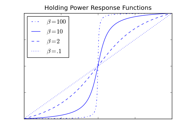
Figure 1: Arctangent provides a smooth blend between step and linear functions.

For very steep parameters this function resembles classification (step function) while for very shallow parameters it resembles a simple linear sum as seen in Fig. 1. We can solve the following optimization problem to maximize the number of vertices, whose positions in the ground-truth clustering are justified by the weighting vector $\alpha$.

$$\arg\max_{\alpha\in\mathbb{R}^{K}}\sum_{v\in V}\arctan(\beta H_{\alpha}(v))$$ (3)

3.2.2 Overall clustering quality

In addition to individual vertices being justified, overall quality of the clustering should be maximized. Any quality metric can potentially be used for this purpose however we find that some strictly linear functions have a trivial solution. Consider an objective function that measures the quality of a clustering as the sum of the inter-cluster edges. To minimize the cumulative weights of cut edges, or equivalently to maximize the cumulative weights of internal edges we solve

$$\min_{\alpha} \sum_{e_{j}\in Cut}\sum_{i=1}^{K}\alpha_{i}w^{i}_{j}\;\;\;|\alpha|=1$$

where $Cut$ denotes the set of edges whose end points are in different clusters. Let $S^{k}$ denote the sum of the cut edges with respect to the $k$-th metric. That is $S^{k}=\sum_{e_{j}\in Cut}w_{j}^{k}$. Then the objective function can be rewritten as $\min_{\alpha}\sum_{1}^{K}\alpha_{k}S^{k}$. Because this is linear it has a trivial solution that assigns 1 to the weight of the maximum $S^{k}$, which means only one similarity metric is taken into account. While additional constraints may exclude this specific solution, a linear formulation of the quality will always yield only a trivial solution within the new feasible region.

In our experiments we used the modularity metric [9]. The modularity metric uses a random graph generated with respect to the degree distribution as the null hypothesis, setting the modularity score of a random clustering to 0. Formally, the modularity score for an unweighted graph is

$$\frac{1}{2m}\sum_{ij}\left[e_{ij}-\frac{d_{i}d_{j}}{4m}\right]\delta_{ij},$$ (4)

where $e_{ij}$ is a binary variable that is 1, if and only if vertices $v_{i}$ and $v_{j}$ are connected; $d_{i}$ denotes the degree of vertex $i$; $m$ is the number of edges; and $\delta_{i,j}$ is a binary variable that is 1, if and only if vertices $v_{i}$ and $v_{j}$ are on the same cluster. In this formulation, $\frac{d_{i}d_{j}}{4m}$ corresponds to the number of edges between vertices $v_{i}$ and $v_{j}$ in a random graph with the given degree distribution, and its subtraction corresponds to the the null hypothesis.

This formulation can be generalized for weighted graphs by redefining $e_{ij}$ as the weight of this edge (0 if no such edge exists), $d_{i}$ as the cumulative weight of edges incident to $v_{i}$; and $m$ as the cumulative weight of all edges in the graph [8].

3.3 Solving the optimization problems

We have presented several nonlinear optimization problems for which the derivative information is not available. To solve these problems we used HOPSPACK (Hybrid Optimization Parallel Search PACKage) [10], which is developed at Sandia National Laboratories to solve linear and nonlinear optimization problems when the derivatives are not available.

4 Experimental results

4.1 Recovering edge weights

The goal of this set of experiments is to see whether we can find aggregation functions that justify a given clustering. We have performed our experiments on 3 data sets.

Synthetic data: Our generation method is based on Lancichinetti et al.’s work [2] that proposes a method to generate graphs as benchmarks for clustering algorithms. We generated networks of sizes 500, 100, 2000, and 4000 nodes, 30 edges per node on average, mixing parameters $\mu_{t}=.7,\mu_{w}=.75$, and known communities. We then perturbed edge weights, $w_{i}$, with additive and multiplicative noise so that $w_{i}\leftarrow\nu(w_{i}+\sigma):\sigma\in(-2w_{a},2w_{a}),\nu\in(0,1)$ uniformly, independently, and identically distributed, where $w_{a}$ is the average edge weight.

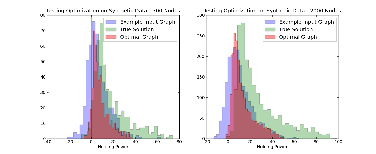
Figure 2: Three histograms of holding powers for Blue: an example perturbed (poor) edge type, Green: the original data (very good), Red: the optimal blend of ten of the perturbed edge types.

After the noise, none of the original metrics preserved the original clustering structure. We display this in Fig. 2, which presents histograms for the holding power for vertices. The green bars correspond to vertices of the original graph, they all have positive holding power. The blue bars correspond to holding powers after noise is added. We only present one edge type for clarity of presentation. As can be seen a significant portion (30%) of the vertices have negative holding power, which means they would rather be on another cluster. The red bars show the holding powers after we compute an optimal linear aggregation. As seen in the figure, almost all vertices move to the positive side, justifying the ground-truth clustering. A few vertices with negative holding power are expected, even after an optimal solution due to the noise. These results show that a composite similarity that resonates with a given clustering can be computed out of many metrics, none of which give a good solution by itself.

In Table 1, we present these results on graphs with different number of vertices. While the percentages change for different number of vertices, our main conclusion that a good clustering can be achieved via a better aggregation function remains valid.

Table 1: Fraction of nodes with positive holding power for ground-truth, perturbed, and optimized networks

Number of nodes	Number of clusters	Ground-truth	Optimized	Perturbed (average)
500	14	.965	.922	.703
1000	27	.999	.977	.799
2000	58	.999	.996	.846
4000	118	1.00	.997	.860

File system data: An owner of a workstation classified 300 of his files as belonging to one of his three ongoing projects, which we took as the ground-truth clustering. We used filename similarity, time-of-modification/time-of-creation similarity, ancestry (distance in the directory-tree), and parenthood (edges between a directory node with file nodes in this directory) as the similarity metrics among these files.

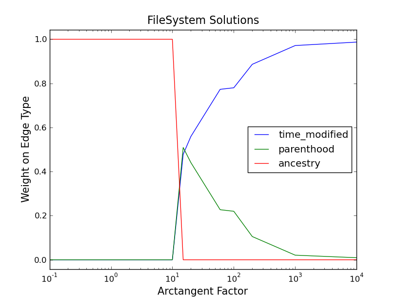
Figure 3: Optimal solutions for the file system data for different arctangent parameters

Our results showed that only three metrics (time-of-modification, ancestry, and parenthood) affected the clustering. However, the solutions were sensitive to the choice of the arctangent parameter. In Fig. 3, each column corresponds to an optimal solution for the corresponding arctangent parameter. Recall that higher values of the arctangent parameter corresponds to sharper step functions. Hence, the right of the figure corresponds to maximizing the total number of vertices with positive holding power, while the left side corresponds to maximizing the sum of holding powers. The difference between the two is that the solutions on the right side may have a lot of nodes with barely positive values, while those on the left may have nodes further away from zero at the cost of more nodes with negative holding power. This is expected in general, but drastic change in the optimal solutions as we go from one extreme to another was surprising to us, and should be taken into account in further studies.

Arxiv data: We took 30,000 high-energy physics articles published on arXiv.org and considered abstract text similarity, title similarity, citation links, and shared authors as edge types for these articles. We used the top-level domain of the submitter’s e-mail (.edu, .uk, .jp, etc…) as a proxy for the region where the work was done. We used these regions as the ground-truth clustering.

The best parameters that explained the ground-truth clustering were 0.0 for abstracts, 1.0 for authors, 0.059 for citations, and 0.0016 for titles. This means the shared authors edge type is almost entirely favored, with cross-citations coming a distant second. This is intuitive because a network of articles linked by common authors will be linked both by topic (we work with people in our field) but also by geography (we often work with people in nearby institutions) whereas edge types like abstract text similarity tend to encode only the topic of a paper, which is less geographically correlated. Different groups can work on the same topic, and it was good to see that citations factored in, and such a clear dominance of the authors information was noteworthy. As a future work, we plan to investigate nonlinear aggregation functions on this graph.

4.2 Clustering quality vs. holding vertices

We have stated two goals while computing an aggregation function: justifying the position of each vertex and the overall quality of clustering. In Fig. 4, we present the Pareto frontier for the two objectives. The vertical axis represent the quality of the clustering with respect to the modularity metric [9], while the horizontal axis represents the percentage of nodes with positive holding power. The modularity numbers are normalized with respect to the modularity of the ground-truth clustering, and normalized numbers can be above 1, since the ground-truth clustering does not specifically aim at maximizing modularity.

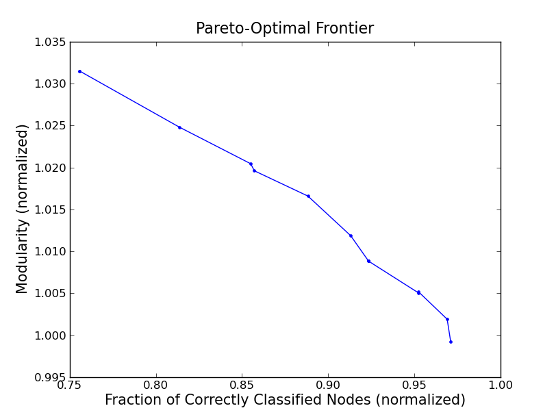
Figure 4: Pareto frontier for two objectives: normalized modularity and percentage of nodes with positive holding power

As expected, Fig. 4 shows a trade-off between two objectives. However, the scale difference between the two axis should be noted. The full range in modularity change is limited to only 3% for modularity, while the range is more than 20% for fraction of vertices with positive holding power. More importantly, by only looking at the holding powers we can preserve the original modularity quality. The reason for this is that we have relatively small clusters, and almost all vertices have a connection with a cluster besides their own. If we had clusters where many vertices had all their connection within their clusters (e.g., much larger clusters), then this would not have been the case, and having a separate quality of clustering metric would have made sense. However, we know that most complex networks have small communities no matter how big the graphs are [4]. Therefore, we expect that looking only at the holding powers of vertices will be sufficient to recover aggregation functions.

4.3 Inverse problems vs. maximizing clustering quality

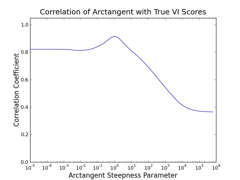
Figure 5: The correlation of the arctan-smoothed objective function with variation of information distance using clusterings generated by Graclus as we vary the steepness parameter

We used the file system data set to investigate the relationship between the two proposed approaches, and present results in Fig. 5. For this figure we compute the objective function for the ground-truth clustering for various aggregation weights and use the same weights to compute clusterings with Graclus. From these clusterings we compute the variation of information (VI) distance to the ground-truth. Fig. 5 presents the correlation between the measures: VI distance for Graclus clusterings for the first approach, and the objective function values for the second approach. This tries to answer whether solutions with higher objective function values yield clusterings closer to the ground-truth using Graclus. In this figure, a horizontal line fixed at 1 would have shown complete agreement. Our results show a strong correlation when moderate values for $\beta$ are taken (arctan function is neither too step-like nor too linear). These results are not sufficient to be conclusive as we need more experiments and other clustering tools. However, this experiment produced promising results and shows how such a study may be performed.

4.4 Runtime scalability

In our final set of experiments we show the scalability of the proposed method. First, we want to note that the number of unknowns for the optimization problem is only a function of the aggregation function and is independent of the graph size. The required number of operations for one function evaluation on the other hand depends linearly on the size of the graph, as illustrated in Figure 6. In this experiment, we used synthetic graphs with 30 as the average degree, and the presented numbers correspond to averages on 10 different runs. As expected, the runtimes scale linearly with the number of edges.

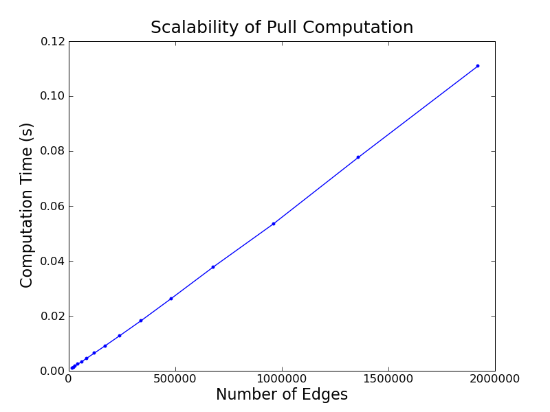
Figure 6: Scalability of the proposed method

The runtime of the optimization algorithm depends on the number of function evaluations. Since the algorithm we used is nondeterministic, the number of function evaluations, hence runtimes vary even for different runs on the same problem, and thus are less informative. We are not presenting these results in detail due to space constraints. However, we want to reemphasize that the size of the optimization problem does not grow with the graph size, and we don’t expect the number of functions evaluations to cause any scalability problems.

We also observed that the number of function evaluations increase linearly with the number of similarity metrics. These results are also omitted due to space constraints.

5 Conclusion and Future Work

We have discussed the problem of graph clustering with multiple edge types, and studied computing an aggregation function to compute composite edge weights that best resonate with given ground-truth clustering. We have applied real and synthetic data sets and presented experimental results that show that our methods are scalable and can recover aggregation functions that yield high-quality clusterings.

This paper only scratches the surface of the clustering problem with multiple edge types. There are many interesting problems to be investigated such as meta-clustering, (i.e., clustering the clusterings) and finding significantly different clusterings for the same data, which are part of our ongoing work. We are also planning to extend our experimental work on the current problem of computing aggregation functions from ground-truth data.

References

- [1] I. Dhillon, Y. Guan, and B. Kulis. Weighted graph cuts without eigenvectors a multilevel approach. IEEE T. pattern analysis and machine intelligence, 29(11):1944–57, 2007.
- [2] Andrea Lancichinetti, Santo Fortunato, and Filippo Radicchi. Benchmark graphs for testing community detection algorithms. Physical Review E, 78(4):046110, October 2008.
- [3] T. Lange, V. Roth, M. L. Braun, and J. M. Buhmann. Stability-based validation of clustering solutions, neural computation. Neural Computation, 16:1299–1323, 2004.
- [4] J. Leskovec, K. Lang, A. Dasgupta, and M. Mahoney. Community structure in large networks: Natural cluster sizes and the absence of large well-defined clusters. Internet Mathematics, 6:29–123, 2009.
- [5] X. Luo. On coreference resolution performance metrics. In Proc. Human Language Technology Conf. and Conf. Empirical Methods in Natural Language Processing, pages 25–32, Vancouver, British Columbia, Canada, 2005. Association for Computational Linguistics.
- [6] M. Meila. Comparing clusterings: an axiomatic view. In 05: Proceedings of the 22nd International Conference on Machine Learning, pages 577–584, 2005.
- [7] B. Mirkin. Mathematical Classification and Clustering. Kluwer Academic Press, 1996.
- [8] M. Newman. Analysis of weighted networks. Phys. Rev. E, 70(5):056131, Nov 2004.
- [9] M. Newman. Modularity and community structure in networks. PNAS, 103:8577–82, 2006.
- [10] T. Plantenga. Hopspack 2.0 user manual. Technical Report SAND2009-6265, Sandia National Laboratories, 2009.
- [11] C. Stichting, M. Centrum, and S. V. Dongen. Performance criteria for graph clustering and markov cluster experiments. Technical Report INS-R0012, Centre for Mathematics and Computer Science, 2000.