Stationary waves in a superfluid exciton gas in quantum Hall bilayers

Abstract

Stationary waves in a superfluid magnetoexciton gas in $\nu=1$ quantum Hall bilayers are considered. The waves are induced by counter-propagating electrical currents that flow in a system with a point obstacle. It is shown that stationary waves can emerge only in imbalanced bilayers in a certain diapason of currents. It is found that the stationary wave pattern is modified qualitatively under a variation of the ratio of the interlayer distance to the magnetic length $d/\ell$. The advantages of use graphene-dielectric-graphene sandwiches for the observation of stationary waves are discussed. We determine the range of parameters (the dielectric constant of the layer that separates two graphene layers and the ratio $d/\ell$) for which the state with superfluid magnetoexcitons can be realized in such sandwiches. Typical stationary wave patterns are presented as density plots.

1 Introduction

Realization of superfluidity of excitons in semiconductor heterostructures is considered as a challenge problem. Exciton mass is smaller or of order of the electron mass and the temperature of the transition into a superfluid state can be quite large. Considerable attention has been given to the superfluidity of spatially indirect excitons in bilayer electron structures. A flow of such excitons results in an appearance of counterflow electrical currents in the layers. They can provide feeding of the load located at one end of the system from the source located at the other end, and superfluidity of spatially indirect excitons can be considered as a kind of unconventional superconductivity. The idea goes back to the papers [1, 2]. This idea was reincarnated in the quantum Hall physics of bilayer electron systems in Refs. [3, 4, 5]. In a quantum Hall bilayer with the total filling factor of Landau levels $\nu_{T}=1$ the state with a spontaneous interlayer phase coherence may emerge (see [6, 7, 8, 9, 10] as a review). The many-particle wave function for such a state describes the pairing of electrons from one layer and holes from the other layer and its structure is analogues to the BCS wave function. Experimental studies of transport properties of quantum Hall bilayers [11, 12, 13, 14, 15] confirm in some part the theoretical prediction. The systems demonstrate vanishing of the Hall resistance and exponential increase of the counterflow conductivity under lowering of temperature. But the conductivity remains finite that can be accounted for unbound vortices [16, 17, 18].

Another hallmark of superfluidity is that an obstacle does not disturb a flowing superfluid at small flow velocity. If the flow velocity exceeds the critical one, the obstacle produces excitations that are in rest relative to it. They are the stationary waves - the waves with the time independent phase in each space point (in the reference frame connected with the obstacle). Stationary waves may emerge in a medium which excitation spectrum has a dispersion. The well-known example is ship waves [19] - the waves produces by a ship on the water surface. The spectrum of deep water waves has negative dispersion and ship waves on a deep water are located behind the floating ship. The Bogolyubov spectrum has positive dispersion and stationary waves in a superfluid weakly non-ideal Bose gas are located outside the Mach cone: the waves appear ahead the obstacle, and do not appear strictly behind it [20].

Stationary waves have been recently observed in an exciton-polariton gas [21]. Since the exciton-polariton mass is much smaller than the electron mass, a two-dimensional exciton-polariton gas in microcavities is considered as a candidate for a high-temperature superfluid [22, 23, 24]. The observation [21] consists in that at rather high exciton-polariton concentration and small flow velocity the waves are not excited. But if the flow velocity exceeds the speed of sound stationary waves emerge outside the Mach cone.

In this paper we consider the possibility of observation of stationary waves in quantum Hall bilayers in a state with a spontaneous interlayer phase coherence. In Sec. 2 we use the kinematic approach [19] based on the analysis of the excitation spectrum and determine the range of the filling factor imbalance and the counterflow currents where stationary waves may emerge. It is found that the stationary wave pattern is modified qualitatively under variation of the ratio of the interlayer distance $d$ to the magnetic length $\ell$. In Sec. 3 we present the description of stationary waves in $\nu_{T}=1$ quantum Hall bilayers in the dynamical approach [19]. The approach allows to compute the amplitudes and phases of stationary wave in each space point. The results are presented as density plots. In Sec. 4 we discuss advantages of use graphene bilayers for the observation of stationary waves.

2 The excitation spectrum and conditions for the emergence of stationary waves in quantum Hall bilayers

In this section we consider under what conditions stationary waves can be excited in a superfluid magnetoexciton gas in bilayers.

We use the kinematic approach [19] that is based on the analysis of the excitation spectrum. The spectrum at general direction of the wave vector relative to the direction of counterflow currents and general filling factor imbalance was obtained in [25, 26] basing on the approach [27]. Here we reproduce in short the derivation [26].

The state with the spontaneous interlayer phase coherence is described by the many-particle wave function [6]

$$|\Psi\rangle=\prod_{X}\left(\cos\frac{\theta_{X}}{2}a^{+}_{1,X}+e^{iQ_{x}X+i\tilde{\varphi}_{X}}\sin\frac{\theta_{X}}{2}a^{+}_{2,X-Q_{y}\ell^{2}}\right)|0\rangle.$$ (1)

Here we use the form of (1) given in Ref. [26]. It corresponds to a coordinate system with the $x$ axis directed at some angle to the counterflow current direction. The quantities $a^{+}_{i,X}$, $a_{i,X}$ are the creation and annihilation operators for the electrons in zeroth Landau level (the lowest Landau level approximation is used), $i$ is the layer index, and $X$ is the guiding center coordinate. The vector-potential is chosen in the form ${\bf A}=(0,Bx,0)$ that corresponds to the single particle wave function $\psi_{X}({\bf r})=(1/\pi^{1/4}\ell)e^{iXy/\ell^{2}}\exp[-(x-X)^{2}/2\ell^{2}]$. The variable $\theta_{X}$ can be presented as a sum of the mean value and the fluctuating part: $\theta_{X}=\theta_{0}+\tilde{\theta}_{X}$. The mean value $\theta_{0}$ is connected with the filling factors by the relation $\cos\theta_{0}=\nu_{1}-\nu_{2}$, where $\nu_{i}=2\pi n_{i}\ell^{2}$ is the filling factor for the $i$-th layer, and $n_{i}$ is the electron concentration. The phase contains the regular $Q_{x}X$ and the fluctuating $\tilde{\varphi}_{X}$ parts.

The counterflow supercurrents are directed along the vector ${\bf Q}=(Q_{x},Q_{y})$. Their values are given by the equation

$${\bf j}_{CF}=\frac{e}{\hbar}\frac{1}{S}\frac{dE_{0}}{d{\bf Q}}.$$ (2)

The quantity ${\bf j}_{CF}$ is defined as the density of the supercurrent in the layer 1 (${\bf j}_{1}=-{\bf j}_{2}={\bf j}_{CF}$), $E_{0}=\langle\Psi_{0}|H_{C}|\Psi_{0}\rangle$ is the mean-field energy for the Hamiltonian of Coulomb interaction in zeroth Landau level in the state (1) at $\tilde{\theta}_{X}=\tilde{\varphi}_{X}=0$, and $S$ is the area of the system.

The explicit expression for $E_{0}$ reads as

$$E_{0}=\frac{S}{8\pi\ell^{2}}\left[\cos^{2}\theta_{0}[H_{0}-F_{S}(0)]-\sin^{2}\theta_{0}{F}_{D}(Q)\right],$$ (3)

where the quantities

$$F_{S(D)}(q)=\frac{1}{2\pi}\int_{0}^{\infty}pJ_{0}(pq\ell^{2})V_{S(D)}(p)e^{-\frac{p^{2}\ell^{2}}{2}}dp$$ (4)

($J_{0}(x)$ is the Bessel function) describe the contribution of the intralayer (S) and the interlayer (D) exchange Coulomb interaction, and the quantity

$$H_{0}=\lim_{q\to 0}\frac{V_{S}(q)-V_{D}(q)}{2\pi\ell^{2}},$$ (5)

the contribution of the direct Coulomb interaction. $V_{S}(q)=2\pi e^{2}/\varepsilon q$ and $V_{D}(q)=2\pi e^{2}e^{-qd}/\varepsilon q$ are the Fourier components of the interaction, and $\varepsilon$ is the dielectric constant.

In the harmonic approximation the energy of fluctuations has the form

$$E_{2}=\sum_{q}[m_{z}(-q)K_{zz}(q)m_{z}(q)+\frac{1}{4}\varphi(-q)K_{\varphi\varphi}(q)\varphi(q)$$ (6)

$$-\frac{1}{2}(im_{z}(-q)K_{z\varphi}(q)\varphi(q)+c.c.)],$$ (7)

where

$${m}_{z}(q)=\frac{1}{2}\sqrt{\frac{2\pi l^{2}}{S}}\sum_{X}\left(\cos\theta_{X}-\cos\theta_{0}\right)e^{-{i}qX},$$ (8)

$${\varphi}(q)=\sqrt{\frac{2\pi l^{2}}{S}}\sum_{X}\tilde{\varphi}(X)e^{-{i}qX}.$$ (9)

The components of the matrix $\bm{K}$ are defined as

$$K_{\alpha\beta}(q)=K_{\alpha\beta}({\bf q})\Big{|}_{{\bf q}=q\mathbf{i}_{x}},$$

where

$$K_{zz}({\bf q})=H({\bf q},{\bf Q})-F_{S}(|{\bf q}|)+F_{D}(|{\bf Q}|)$$ (10)

$$+\left(F_{D}(|{\bf Q}|)-\frac{F_{D}(|\mathbf{q}+\mathbf{Q}|)+F_{D}(|\mathbf{q}-\mathbf{Q}|)}{2}\right)\cot^{2}\theta_{0},$$ (11)

$$K_{\varphi\varphi}({\bf q})=\sin^{2}\theta_{0}\left[F_{D}(|{\bf Q}|)-\frac{F_{D}(|\mathbf{q}+\mathbf{Q}|)+F_{D}(|\mathbf{q}-\mathbf{Q}|)}{2}\right],$$ (12)

$$K_{z\varphi}({\bf q})=-\cos\theta_{0}\frac{F_{D}(|\mathbf{q}+\mathbf{Q}|)-F_{D}(|\mathbf{q}-\mathbf{Q}|)}{2},$$ (13)

and

$$H({\bf q},{\bf Q})=\frac{1}{2\pi\ell^{2}}\left[V_{S}(|{\bf q}|)-V_{D}(|{\bf q}|)\cos\left(|\mathbf{q}\times\mathbf{Q}|\ell^{2}\right)\right]e^{-\frac{q^{2}\ell^{2}}{2}}.$$ (14)

The quantities $\hbar m_{z}(q)$ and $\varphi(-q)$ are the conjugated variables. It can be checked by computing the commutator of the operators that correspond to these variables. The canonical equations of motion read as

$$\hbar\frac{d{\varphi}(q)}{dt}=2K_{zz}(q){m}_{z}(q)-iK_{z\varphi}(q){\varphi}(q),$$ (15)

$$\hbar\frac{d{m}_{z}(q)}{dt}=-\frac{1}{2}K_{\varphi\varphi}(q){\varphi}(q)-iK_{z\varphi}(q){m}_{z}(q).$$ (16)

According to Eq. (15) the energy of the collective mode with the wave vector ${\bf q}=q{\bf i}_{x}$ has the form $\Omega(q)=\sqrt{K_{\varphi\varphi}(q)K_{zz}(q)}+K_{z\varphi}(q)$. Rotating the axes we find the excitation spectrum at general ${\bf q}$

$$\Omega({\bf q})=\sqrt{K_{\varphi\varphi}({\bf q})K_{zz}({\bf q})}+K_{z\varphi}({\bf q}).$$ (17)

In what follows we use the reference frame with the $x$ axis directed along ${\bf Q}$ (${\bf Q}=(Q,0)$) that coincides with the direction of the current ${\bf j}_{CF}$ Eq. (2).

The wave vectors for the stationary waves satisfy the equation

$$\Omega({\bf q}_{st})=0.$$ (18)

The necessary condition for the observation of stationary waves is the existence of nontrivial solutions of Eq. (18). Beside that, the spectrum $\Omega({\bf q})$ should be real valued at all ${\bf q}$ (complex valued $\Omega({\bf q})$ signal for the dynamical instability of the state Eq. (1)). These two conditions determine the parameters of the systems where stationary waves can emerge.

The spectrum (17) depends on three parameters: the ratio $\tilde{d}=d/\ell$, the filling factor imbalance $\tilde{\nu}=(\nu_{1}-\nu_{2})/2$ and the gradient of the phase $Q$. The spectrum should be real valued at $Q=0$. It gives the restriction $\tilde{d}<\tilde{d}_{c}(\tilde{\nu})$. The dependence $\tilde{d}_{c}(\tilde{\nu})$ is shown in Fig. 1. The stationary wave equation (18) has nontrivial solutions at $Q>Q_{1}(\tilde{d},\tilde{\nu})$. On the other hand, the condition for the quantity $\Omega({\bf q})$ be real valued at all ${\bf q}$ yields the restriction $Q<Q_{2}(\tilde{d},\tilde{\nu})$ ($Q_{1}\leq Q_{2}$) Thus, stationary waves can be observed at $Q_{c1}<Q<Q_{c2}$ that corresponds to $j_{c1}<j_{CF}<j_{c2}$. The quantities $j_{c1}$ and $j_{c2}$ are the function of $\tilde{d}$ and $\tilde{\nu}$. The dependences $j_{c1}$ and $j_{c2}$ on the filling factor imbalance are shown in Fig. 2 (these dependences are symmetric with respect to $\tilde{\nu}$ and we present them only for $\tilde{\nu}>0$) On can see from Fig. 2 that in balanced bilayers ($\tilde{\nu}=0$) the diapason of currents at which stationary waves can be excited shrinks to zero.

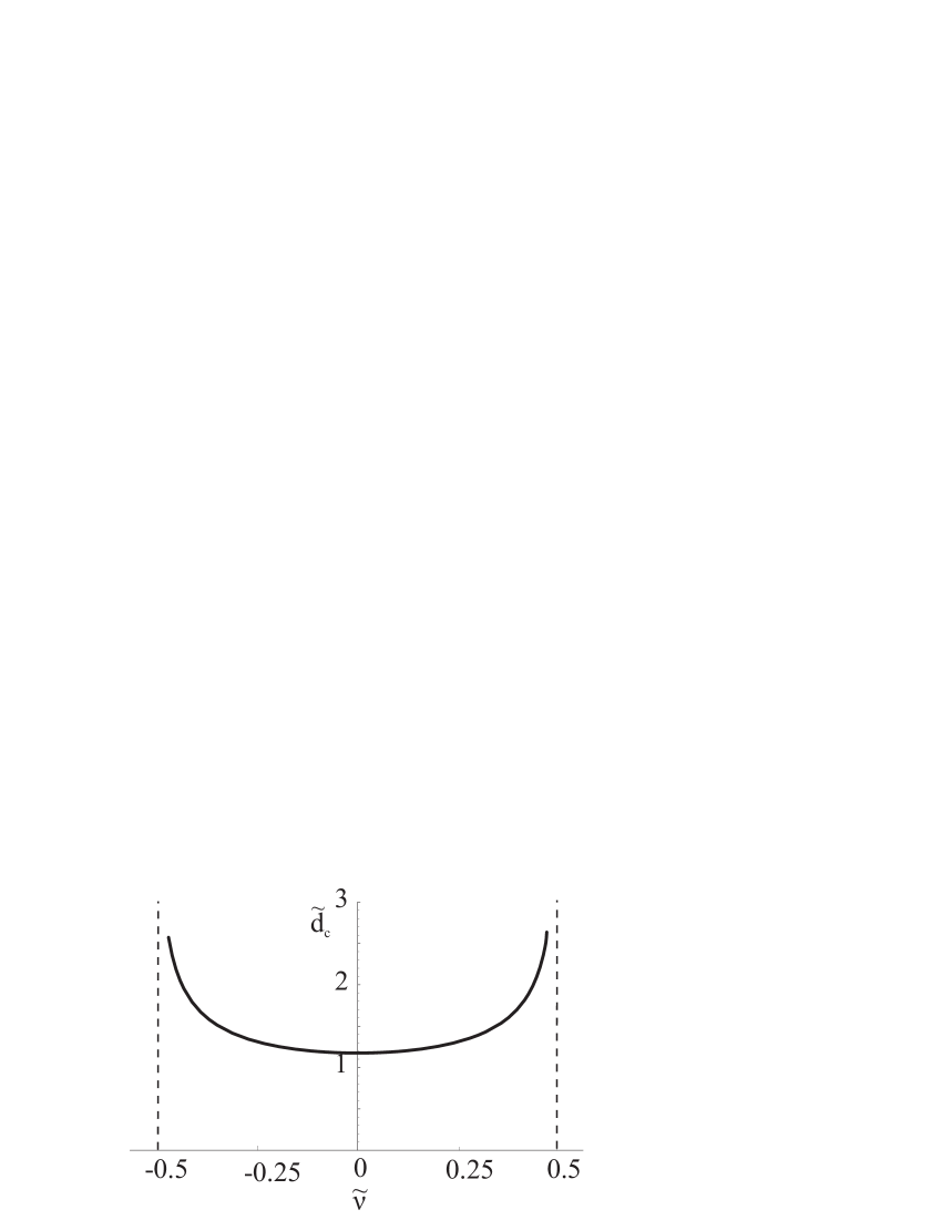
Figure 1: Critical interlayer distance versus the filling factor imbalance

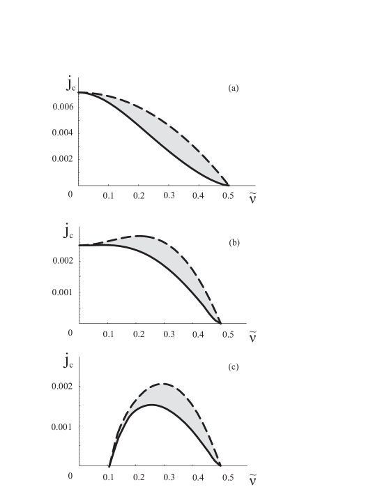
Figure 2: The critical currents $j_{c1}$ (solid line) and $j_{c2}$ (dashed line) at $d/\ell=0.3$ (a), $d/\ell=1.1$ (b), and $d/\ell=1.2$ (c). The current density $j$ is in $e^{3}/\hbar\varepsilon\ell^{2}$ units. The range of currents and filling factor imbalance where stationary waves are excited is shown grey.

The existence of two critical currents $j_{c1}$ and $j_{c2}$ reflects the general situation in superfluid systems. The existence of Landau critical velocity (that in our case corresponds to the current $j_{c1}$) is a common feature of superfluid systems. While a single component uniform Bose-Einstein condensate does not demonstrate the dynamical instability, more complex superflud systems do. The examples are superfluid Bose-Einstein condensates in a lattice [28, 29], phase-separated two-component superfluid, where the components have a common interface [30, 31], and two-component superfluid mixtures (with penetrating components) [32, 33, 34].

In general case the Landau critical velocities are smaller than ones that cause the dynamical instability, but in some cases the system switches directly to the dynamical instability regime. As was shown in [32], such a situation takes place in a symmetric two-component Bose-Einstein condensate (two components with the same characteristics) if the components flow with equal velocities in opposite directions. In the latter case, in similarity with a situation in balanced quantum Hall bilayers, there is no range of velocities where stationary wave pattern may emerge. Such a similarity can be understood as follows. In a quantum Hall bilayer with $\nu_{T}=1$ the exciton transport can be interpreted as counter-propagation of two exciton species of different polarization, and in balanced bilayers such species move in opposite directions with the same velocities.

The dynamical instability means that the magnetoexciton state is unstable irrespectively to the interaction of magnetoexcitons with an environment. The interaction with an environment may result in a Landau (thermodynamic) instability in superfluids that develops under the flow with the velocities larger than the Landau critical velocities [30, 35]. Phenomenologically, such type of instability can be described by a modified Gross-Pitaevskii equation that includes a dissipative term [35]. Microscopically, the dissipative term can be connected with an interaction between the condensate and normal components in a state where these two component are out of equilibrium with each other, and the normal component interacts with an environment [36, 37]. As was shown in [31, 35], the Landau instability may reveal itself in a vortex nucleation at the interface between two superfluid. In a typical situation the Landau instability is much weaker than the dynamical instability. In our study we do not take into account the Landau instability effects implying that the system is in a regime where such effects are small.

The quantity $K_{z\varphi}({\bf q})$ in the spectrum (17) contains the factor $\cos\theta_{0}$ which sign coincides with the sign of the filling factor imbalance. Therefore at $\nu_{1}>\nu_{2}$ the stationary wave equation (18) can be satisfied for the wave vectors that have negative projection on the direction of ${\bf Q}$ ($q_{x}<0$), and at $\nu_{1}<\nu_{2}$, for the wave vectors with $q_{x}>0$. In systems that differ only by a sign of the imbalance the stationary wave patterns will be the mirror images of each other.

To be more specific we consider below the case $\nu_{1}>\nu_{2}$. It is convenient to parameterize the stationary wave crests by the angle $\xi$ that determines the direction of the wave vector counted from the $-x$ axis: ${\bf q}_{st}=(-q\cos\xi,q\sin\xi)$. At $\nu_{1}>\nu_{2}$ the Mach cone is situated in the $x>0$ half-plane and the Mach angle is $\alpha_{M}=\pi/2-\xi_{M}$, where $\xi_{M}$ is the maximum angle of deviation of ${\bf q}_{st}$ from the $-x$ direction.

Eq. (18) can be considered as an implicit definition of the function $q_{st}(\xi)$. In general case this equation has several solutions $q_{st,\lambda}(\xi)$, where the index $\lambda$ numerates different families of stationary waves.

To each wave vector ${\bf q}_{st}$ one can put in correspondence the group velocity vector

$${\bf v}_{g}=\frac{1}{\hbar}\frac{\partial\Omega({\bf q})}{\partial{\bf q}}\Bigg{|}_{{\bf q}={\bf q}_{st}}.$$ (19)

The polar angle $\chi$ that determines the direction of the group velocity ${\bf v}_{g}$ relative to the $x$ axis is also the function of $\xi$. The dependence $\chi(\xi)$ can be obtained from Eq. (19) under substitution ${\bf q}_{st}=(-q_{st}(\xi)\cos\xi,q_{st}(\xi)\sin\xi)$.

A point defect located at the origin emits stationary waves. Their phase at the space point ${\bf r}$ is equal to

$$\theta={\bf q}_{st}\cdot{\bf r}=-q_{st}(\xi)r\cos[\xi+\chi(\xi)].$$ (20)

The latter equation gives the dependence $r(\xi,\theta)$. The coordinates of the wave crests can be presented in the parametric form

$$x(\xi,\theta)=-\frac{\theta\cos[\chi(\xi)]}{q_{st}(\xi)\cos[\xi+\chi(\xi)]},$$ (21)

$$y(\xi,\theta)=-\frac{\theta\sin[\chi(\xi)]}{q_{st}(\xi)\cos[\xi+\chi(\xi)]}.$$ (22)

The parameter $\xi$ belongs to the interval $|\xi|<\xi_{M}$. The phase takes the values $\theta=\pm 2\pi N+\theta_{in}$, where $N=1,2,\ldots$, and $\theta_{in}$ is some initial phase that cannot be determined in the kinematic approach (for the calculations we put $\theta_{in}=0$). The sign of $\theta$ is the same for a given family of waves and can be found from the condition $r(\xi,\theta)>0$ that is equivalent to $\theta\cos[\xi+\chi(\xi)]<0$.

As was mentioned in Introduction, the location of stationary waves is determined by the type of dispersion of the collective mode. In the case considered the dispersion depends on the parameter $\tilde{d}$. Typical dispersion curves at $Q=0$ are shown in Fig. 3. One can see that at rather small $\tilde{d}$ the dispersion is positive at all $q$. At larger $\tilde{d}$ the dispersion becomes negative at intermediate $q$. At $\tilde{d}$ close to critical one the spectrum contain a minimum at finite $q$. The wave crests obtained for these three cases are shown in Fig. 4. One can see that in the case of small $\tilde{d}$ the stationary wave pattern is similar to one that was predicted and observed in weakly non-ideal superfluid Bose gases, while at larger $\tilde{d}$ an additional family of stationary waves emerges inside the Mach cone. The minimum in the spectrum reveals itself in an appearance of cusps on the crest lines.

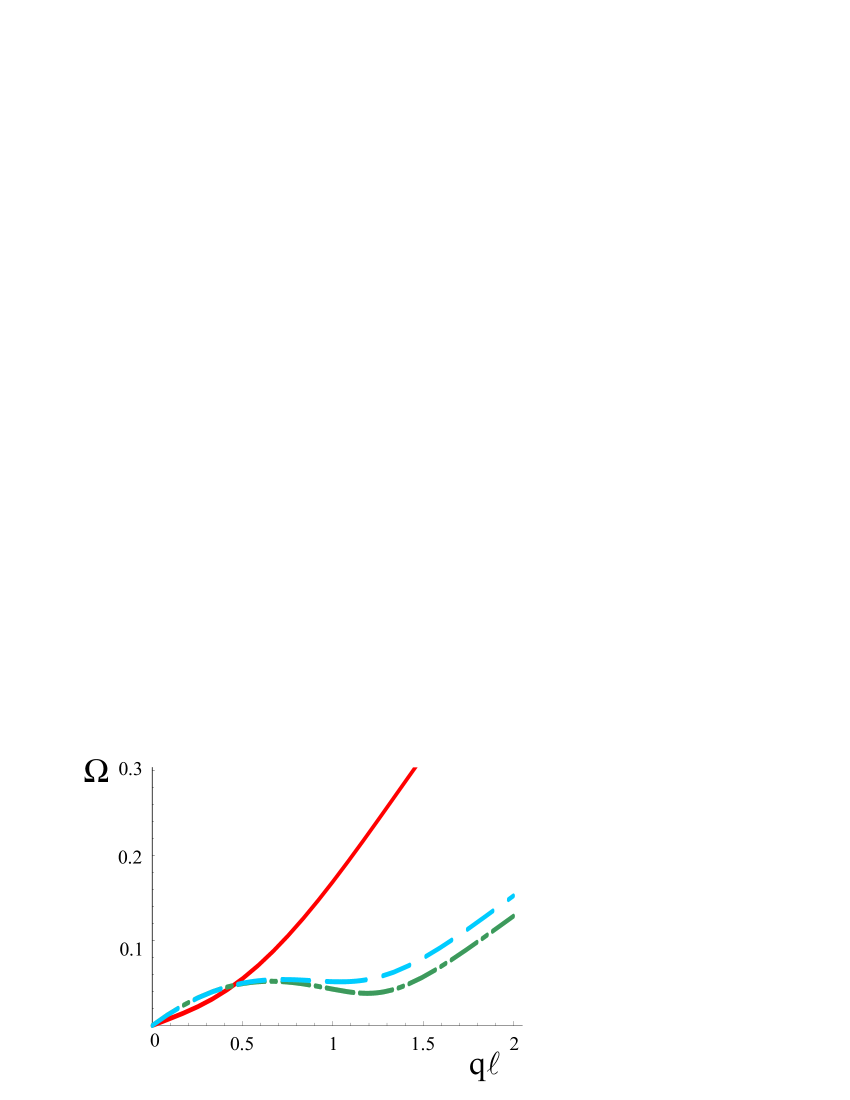
Figure 3: The spectrum of collective excitations (in $e^{2}/\varepsilon\ell$ units) at $d/\ell=0.3$ (solid line), $d/\ell=1.1$ (dashed line) and $d/\ell=1.2$ (dash-and-dot line) for the filling factor imbalance $\tilde{\nu}=0.25$.

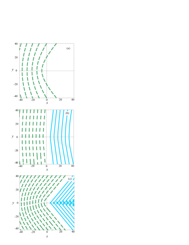
Figure 4: Stationary wave crests at $\tilde{\nu}=0.25$ and (a) — $d/\ell=0.3$, $j_{CF}=4.5\cdot 10^{-3}e^{3}/\hbar\varepsilon\ell^{2}$; (b) — $d/\ell=1.1$, $j_{CF}=2.2\cdot 10^{-3}e^{3}/\hbar\varepsilon\ell^{2}$; (c) — $d/\ell=1.2$, $j_{CF}=1.9\cdot 10^{-3}e^{3}/\hbar\varepsilon\ell^{2}$. The family located outside (inside) the Mach cone is shown by dashed (solid) lines. The spatial scale is $1=\ell$.

3 Stationary wave patters in a superfluid magnetoexciton gas

To compute the amplitudes of stationary waves we will use the dynamical approach [19]. Stationary waves emerge as a response on an obstacle that was appeared in the past. The casuality principle can be realized by the following choice for the Hamiltonian of interaction with the obstacle

$$H_{int}=\int d^{2}re^{\eta t}\sum_{i}V_{i}({\bf r})\rho_{i}({\bf r}),$$ (23)

where $V_{i}({\bf r})$ ($i=1,2$) is the interaction potential, $\rho_{i}({\bf r})$ is the electron density operator, and $\eta=+0$. We consider the point obstacle $V_{i}({\bf r})=U_{i}\delta({\bf r})$ and imply that the interaction (23) does not change the sum of local filling factors of the layers.

In the state (1) the energy of the interaction (23) reads as

$$E_{int}=\frac{U_{z}e^{\eta t}}{S}\sum_{q}\sum_{X}\cos\theta_{X}\frac{1+e^{iqQ_{y}\ell^{2}}}{4}e^{-iqX-\frac{q^{2}\ell^{2}}{4}},$$ (24)

where $U_{z}=U_{1}-U_{2}$. The fluctuating part of (24) expressed in terms of $m_{z}(q)$ has the form

$$E_{int}^{fl}=\frac{U_{z}e^{\eta t}}{\sqrt{2\pi\ell^{2}S}}\sum_{q}m_{z}(q)\frac{1+e^{iqQ_{y}\ell^{2}}}{2}e^{-\frac{q^{2}\ell^{2}}{4}}.$$ (25)

The interaction (25) modifies the equations of motion:

$$\hbar\frac{d{\varphi}(q)}{dt}=2K_{zz}(q){m}_{z}(q)-iK_{z\varphi}(q){\varphi}(q)+\frac{U_{z}e^{\eta t}}{\sqrt{2\pi\ell^{2}S}}\frac{1+e^{-iqQ_{y}\ell^{2}}}{2}e^{-\frac{q^{2}\ell^{2}}{4}},$$ (26)

$$\hbar\frac{d{m}_{z}(q)}{dt}=-\frac{1}{2}K_{\varphi\varphi}(q){\varphi}(q)-iK_{z\varphi}(q){m}_{z}(q).$$ (27)

Taking the partial solution of (26) at $t=0$, we obtain the following expression for $m_{z}(q)$

$$m_{z}(q)=-\frac{U_{z}}{4\sqrt{2\pi\ell^{2}S}}\frac{K_{\varphi\varphi}(q)(1+e^{-iqQ_{y}\ell^{2}})e^{-\frac{q^{2}\ell^{2}}{4}}}{K_{zz}(q)K_{\varphi\varphi}(q)-(K_{z\varphi}(q)-i\hbar\eta)^{2}}.$$ (28)

Using the inverse Fourier transformation for $m_{z}(q)$

$$\cos\theta_{X}=\cos\theta_{0}+2\sqrt{\frac{2\pi\ell^{2}}{S}}\sum_{q}m_{z}(q)e^{iqX},$$ (29)

the expression for the Fourier component of the electron density difference

$$\rho_{1}({\bf q})-\rho_{2}({\bf q})=\delta_{q_{y},0}\sum_{X}\cos\theta_{X}\frac{1+e^{iq_{x}Q_{y}\ell^{2}}}{2}e^{-iq_{x}X-\frac{q^{2}\ell^{2}}{4}},$$ (30)

and taking the inverse Fourier transformation of (30)

$$\Delta\rho({\bf r})=\rho_{1}({\bf r})-\rho_{2}({\bf r})=\frac{1}{S}\sum_{\bf q}\left[\rho_{1}({\bf q})-\rho_{2}({\bf q})\right]e^{i{\bf q}\cdot{\bf r}},$$ (31)

we obtain

$$\Delta\rho({\bf r})=\frac{\cos\theta_{0}}{2\pi\ell^{2}}-\frac{U_{z}}{2\pi\ell^{2}}\frac{1}{2S}\sum_{\bf q}e^{i{\bf q}\cdot{\bf r}}\delta_{q_{y},0}\frac{K_{\varphi\varphi}(q)[1+\cos(q_{x}Q_{y}\ell^{2})]e^{-\frac{q^{2}\ell^{2}}{2}}}{K_{zz}(q)K_{\varphi\varphi}(q)-(K_{z\varphi}(q)-i\hbar\eta)^{2}}$$ (32)

The first term in Eq. (32) is the uniform electron density imbalance $\Delta\rho_{0}$. The nonuniform part $\tilde{\rho}=\Delta\rho-\Delta\rho_{0}$ describes the density fluctuations caused by the stationary waves. Eq. (32) yields the contribution of the modes with the wave vectors directed along the $x$ axis. The contribution of modes with general ${\bf q}$ can be obtained by rotation of the coordinate axes. Summing the contribution of all ${\bf q}$ we find

$$\tilde{\rho}({\bf r})=-\frac{U_{z}}{2\pi\ell^{2}}\frac{1}{2S}\sum_{\bf q}e^{i{\bf q}\cdot{\bf r}}\frac{K_{\varphi\varphi}({\bf q})[1+\cos(|{\bf q}\times{\bf Q}|\ell^{2})]e^{-\frac{q^{2}\ell^{2}}{2}}}{K_{zz}({\bf q})K_{\varphi\varphi}({\bf q})-(K_{z\varphi}({\bf q})-i\hbar\eta)^{2}}.$$ (33)

Replacing the sum with the integral and using the symmetry properties of (33) we obtain

$$\tilde{\rho}(\mathbf{r})=-\frac{U_{z}}{2\pi l^{2}}\frac{1}{(2\pi)^{2}}\textrm{Re}\int_{\frac{-\pi}{2}}^{\frac{\pi}{2}}d\xi\int_{0}^{\infty}dqe^{-iqr\cos(\xi+\chi)}I(q,\xi),$$ (34)

where

$$I(q,\xi)=\frac{qK_{\varphi\varphi}(q,\xi)[1+\cos(qQ\ell^{2}\sin\xi)]e^{-\frac{q^{2}l^{2}}{2}}}{K_{zz}(q,\xi)K_{\varphi\varphi}(q,\xi)-(K_{z\varphi}(q,\xi)-i\hbar\eta)^{2}},$$ (35)

and $\chi$ is the polar angle for the vector ${\bf r}$.

The integral over $q$ in Eq. (34) is evaluated from the residue theorem. The integration contour is chosen as shown in Fig. 5. The contour 1 in Fig. 5 corresponds to the case where the observation point is outside the Mach cone, and the contour 2, inside the Mach cone. The integral along the imaginary axis yields the contribution of order $(r\ell)^{-2}$, while the integral along the real axis - the contribution of order $(r\ell)^{-1/2}$. We specify the case $r\ell\gg 1$ for which the first contribution can be neglected. In this approximation

$$\tilde{\rho}(\mathbf{r})\approx\frac{U_{z}}{2\pi l^{2}}\frac{1}{2\pi}\textrm{Im}\int_{\frac{-\pi}{2}}^{\frac{\pi}{2}}d\xi\sum_{\lambda}s_{\lambda}e^{-iq_{\lambda}(\xi)r\cos(\xi+\chi)}{\rm Res}_{q=q_{\lambda}(\xi)}[I(q,\xi)],$$ (36)

where $q_{\lambda}(\xi)$ are the poles of $I(q,\xi)$, and the factor

$$s_{\lambda}=\left\{\begin{array}[]{ll}1,&\hbox{$\cos(\xi+\chi){\rm Im}(q_{\lambda}(\xi))<0$}\\ 0,&\hbox{$\cos(\xi+\chi){\rm Im}(q_{\lambda}(\xi))>0$}\\ \end{array}\right.$$ (37)

indicates whether is the pole $q_{\lambda}(\xi)$ inside or outside the contour of integration Fig. 5.

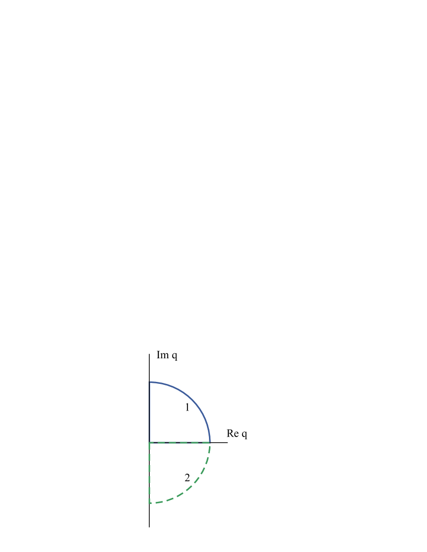
Figure 5: The integration contours used for the computation of the integral (34)

The integral over $\xi$ is evaluated in the stationary phase approximation

$$\tilde{\rho}(\mathbf{r})\approx\frac{U_{z}}{2\pi l^{2}}\sum_{\lambda}\sum_{\xi_{i}}A_{\lambda}(\xi_{i})\frac{\sin\left[q_{\lambda}(\xi_{i})r\cos(\chi+\xi_{i})+\frac{\pi}{4}{\rm sgn}[g_{\lambda}(\xi_{i})]\right]}{\sqrt{r}}.$$ (38)

Here $\xi_{i}$ are the solutions of the stationary phase equation

$$\frac{d}{d\xi}\left[q_{\lambda}(\xi)\cos(\chi+\xi)\right]=0,$$ (39)

the function $g_{\lambda}(\xi)$ is defined as

$$g_{\lambda}(\xi)=\frac{d^{2}}{d\xi^{2}}\left[q_{\lambda}(\xi)\cos(\chi+\xi)\right],$$ (40)

and the amplitude $A_{\lambda}(\xi)$ is equal to

$$A_{\lambda}(\xi)=-s_{\lambda}\sqrt{\frac{1}{2\pi|g_{\lambda}(\xi)|}}{\rm Res}_{q=q_{\lambda}(\xi)}[I(q,\xi)].$$ (41)

One can check that Eq. (38) up to the initial phase yields the same wave crests as determined by the parametric equations (21). Indeed, in the limit $\eta\to 0$ the poles $q_{\lambda}(\xi)$ coincide with the stationary wave vectors determined by Eq. (18). The stationary phase equation (39) determines the multi-valued function $\xi_{i}(\chi)$ that is reciprocal to the function $\chi(\xi)$ defined by Eq. (19). Let us prove the last statement. Considering $q$ and $\xi$ as independent variables one finds

$$\frac{\partial\Omega}{\partial q_{x}}=-\frac{\partial\Omega}{\partial q}\cos\xi-\frac{\partial\Omega}{\partial\xi}\frac{\sin\xi}{q}$$ (42)

$$\frac{\partial\Omega}{\partial q_{y}}=\frac{\partial\Omega}{\partial q}\sin\xi+\frac{\partial\Omega}{\partial\xi}\frac{\cos\xi}{q}$$ (43)

Taking into account the relation

$$\frac{\partial\Omega}{\partial q}\Bigg{|}_{q=q_{st}(\xi)}q_{st}^{\prime}(\xi)+\frac{\partial\Omega}{\partial\xi}\Bigg{|}_{q=q_{st}(\xi)}=0$$

and Eqs. (19),(42) we obtain

$$\tan\chi=\frac{\sin\xi-\frac{q^{\prime}}{q}\cos\xi}{-\cos\xi+\frac{q^{\prime}}{q}\sin\xi}$$ (44)

that yields

$$\tan(\chi+\xi)=\frac{q_{st}^{\prime}(\xi)}{q_{st}(\xi)}$$ (45)

Eq. (45) is equivalent to Eq. (39). Note that Eq. (45) gives the explicit expression for the function $\xi(\chi)$ that can be used instead of the implicit expression (19) for the computation of the wave crest lines.

The stationary wave density pattern given by Eq. (38) is shown in Fig. 6. For the computations we use the same parameters as in Fig. 4c.

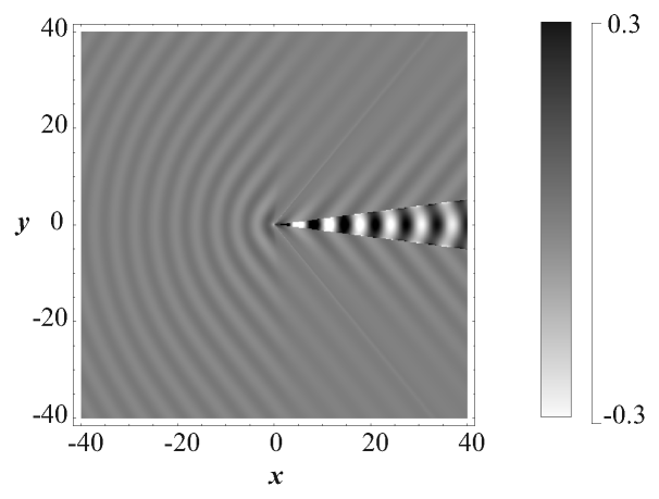
Figure 6: The stationary wave density pattern for the spectrum with a minimum at finite $q$. The density difference is given in $U_{z}/2\pi\ell^{2}E_{C}$ units, where $E_{C}=e^{2}/\varepsilon\ell$ is the Coulomb energy. The spatial scale is $1=\ell$.

4 Stationary density waves in a graphene-dielectric-graphene sandwich

Stationary waves in quantum Hall bilayers reveal itself in spatially non-uniform local electrical fields that emerge due to variations of electron densities in the layers. The period of stationary waves is proportional to the magnetic length. For typical magnetic fields used for the study of magnetoexciton superfluidity in GaAs heterostructures magnetic length is of order of 10 nm that corresponds to the stationary wave period less than $100$ nm (see Fig. 6). For the observation of stationary waves an electrostatic field detector should be located close to the electron layer and its spatial resolution should be smaller than the stationary wave period.

In this section we discuss advantages of use bilayer graphene structures for the observation of stationary waves in the magnetoexciton gas. The problem of exciton superfluidity in double-layer graphene structures was studied theoretically in a number of papers [26, 38, 39, 40, 41, 42]. Here we follow the paper [26], where the theory of magnetoexciton superfluidity in graphene bilayers was developed.

In difference with quantum wells, the graphene layers can be located at the surface of the system. It was reported recently on the creation of a bilayer graphene structure that has one open layer and separate contacts in each layers [43].

Another advantage of graphene systems is much larger energy distance between Landau levels in comparison with one for quantum wells in GaAs heterostructures. That allows to use smaller magnetic fields. Smaller field correspond to larger magnetic length and larger spatial period of stationary waves in absolute units.

Let us discuss this question in a more quantitative way. The energies of Landau levels in graphene are given by the expression [44]

$$E_{\rm LL}(N)={\rm sgn}(N)\frac{\hbar v_{F}\sqrt{2|N|}}{\ell},$$ (46)

where $N$ is integer number, and $v_{F}=10^{6}$ m/s is the Fermi velocity for graphene. Landau levels in graphene have the additional fourfold degeneracy (four components correspond to different combinations of spin and valley indices). In a free-standing graphene the $N=0$ level is half-filled, but in difference with the single component systems magnetoexciton superfluidity in the graphene bilayers is not possible at half-filling [26].

The situation is similar to ones for $\nu_{T}=2$ double quantum wells [45]. Electrostatic field applied perpendicular to the graphene layers may create an imbalance of filling of $N=0$ Landau level in the layers 1 and 2. We consider the cases $\nu_{1}=2+\nu_{a}$, $\nu_{2}=2-\nu_{a}$, and $\nu_{1}=3+\nu_{a}$, $\nu_{2}=1-\nu_{a}$ ($0<\nu_{a}<1$). Here the filling factors are defined as the average number of filled quantum states in a given level per the area $2\pi\ell^{2}$. The quantities $\nu_{a1}=\nu_{a}$ and $\nu_{a2}=1-\nu_{a}$ give the filling factors for the so called active component: only for one (active) component the modulus of the order parameter for the electron-hole pairing is nonzero: $|\Delta_{a}|=\sqrt{\nu_{a}(1-\nu_{a})}$.

The eigenfunction for the zero Landau level in graphene coincides with the eigenfunction for free electron gas. That is why the dynamics of the active component in the bilayer graphene system is described by basically the same equations that were used in the previous section.

Here we consider the graphene-dielectric-graphene sandwich structure with two open graphene layers (two layers separated by a dielectric layer which thickness is much larger than the distance between graphenes in graphite). For such a structure the Fourier components of the intralayer and interlayer Coulomb interaction read as

$$V_{S}(q)=\frac{4\pi e^{2}}{q}\frac{(\varepsilon+1)e^{qd}+(\varepsilon-1)e^{-qd}}{(\varepsilon+1)^{2}e^{qd}-(\varepsilon-1)^{2}e^{-qd}},$$ (47)

$$V_{D}(q)=\frac{2\pi e^{2}}{q}\frac{4\varepsilon}{(\varepsilon+1)^{2}e^{qd}-(\varepsilon-1)^{2}e^{-qd}}.$$ (48)

The dielectric constant for the environment $\varepsilon_{en}=1$ is assumed.

The empty states in a partially filled Landau level can be considered as holes if the Coulomb interaction energy is smaller than the energy distance between Landau levels. Let us use the inequality

$$F_{S}(0)<E_{LL}(1)-E_{LL}(0)=\frac{\sqrt{2}\hbar v_{F}}{\ell}$$ (49)

as a quantitative condition of smallness of the Coulomb interaction. The quantity $F_{S}(0)$ determines the strength of the intralayer exchange interaction. The right hand part of Eq. (49) is the distance between the active ($N=0$) and the nearest passive ($N=\pm 1$) Landau level for graphene. For the geometry considered in [26] (two graphene layers embedded in a dielectric matrix) the quantity $F_{S}(0)=\sqrt{\pi/2}e^{2}/\varepsilon\ell$ and the inequality (49) yields the restriction only of the dielectric constant ($\varepsilon>2$). For the graphene-dielectric-graphene sandwich the intralayer exchange energy depends on $\tilde{d}$:

$$F_{S}(0)=\frac{e^{2}}{\ell}\int_{0}^{\infty}dxe^{-\frac{x^{2}}{2}}\frac{2[(\varepsilon+1)e^{x\tilde{d}}+(\varepsilon-1)e^{-x\tilde{d}}]}{(\varepsilon+1)^{2}e^{x\tilde{d}}-(\varepsilon-1)^{2}e^{-x\tilde{d}}}$$ (50)

and the inequality (49) yields the restriction $\tilde{d}>\tilde{d}_{c1}(\varepsilon)$, where the function $\tilde{d}_{c1}(\varepsilon)$ is given implicitly by the equation $F_{S}(0)={\sqrt{2}\hbar v_{F}}/\ell$. On the other hand, the condition for the excitation spectrum be real valued yields another restriction on the parameter $\tilde{d}$: $\tilde{d}<\tilde{d}_{c}(\tilde{\nu}_{a},\varepsilon)$, where $\tilde{\nu}_{a}=\nu_{a}-1/2$ is the imbalance for the active component. In difference with the situation shown in Fig. 1 the critical distance $\tilde{d}_{c}$ for the graphene-dielectric-graphene sandwich structure depends on the dielectric constant. The dependences $\tilde{d}_{c}(\varepsilon)$ and $\tilde{d}_{c1}(\varepsilon)$ are shown in Fig. 7. One can see that $\tilde{d}_{c1}<\tilde{d}_{c}$ for $\varepsilon\gtrsim 4$ and under appropriate choice of $d/\ell$ one can satisfy the both restriction. At fixed $d$ the magnetic length is restricted from above and from below, but the diapason of allowed $\ell$ can be shifted by a change of $d$. Thus, one can adjust the parameters to make the period of stationary waves appropriate for the observation.

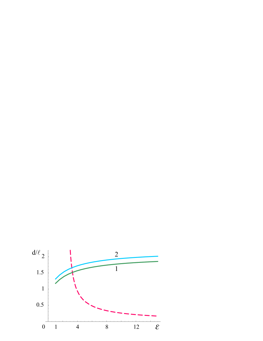
Figure 7: Critical interlayer distance $d_{c}$ (solid lines 1 – $\tilde{\nu}_{a}=0$, solid lines 2 – $\tilde{\nu}_{a}=0.25$) and $d_{c1}$ (dashed line) for the graphene-dielectric-graphene sandwich structure.

In Fig. 8 we present the stationary wave density pattern computed for a graphene-dielectric-graphene structure. The cases of one family and two families without cusps are shown. One can see from the Figs. 6 and 8a,b that the amplitude of stationary waves grows up when $d$ approaches to $d_{c}$.

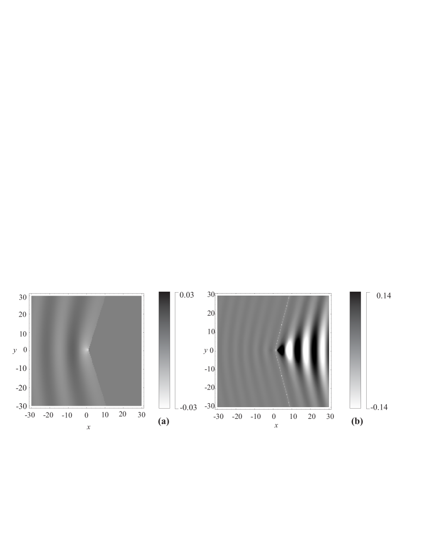
Figure 8: Stationary wave patterns in a graphene-dielectric-graphene sandwich structure with $\varepsilon=15$ and $\tilde{\nu}_{a}=0.25$. (a) – $d/\ell=1.1$, $j_{CF}=1.1\cdot 10^{-2}e^{3}/\hbar\varepsilon\ell^{2}$; (b) – $d/\ell=1.5$, $j_{CF}=6.9\cdot 10^{-3}e^{3}/\hbar\varepsilon\ell^{2}$

5 Conclusion

In conclusion, we wave studied stationary waves in a magnetoexciton gas in quantum Hall bilayers. Stationary waves are static excitations of the difference of electron densities in the layers. They are induced by the counter-propagating electrical currents flowing in a system with an obstacle. It is found that such waves can be excited only in imbalanced bilayers in a certain range of currents. The stationary wave pattern is modified qualitatively under a variation of the ratio of the interlayer distance to the magnetic length $d/\ell$. At small $d/\ell$ the pattern is similar to one that emerges in a superfluid weakly non-ideal Bose gas: stationary waves are located outside the Mach cone. At larger $d/\ell$ an additional family of waves is located inside the Mach cone appears. Under further increase of $d/\ell$ cusps are developed in the crests that correspond to the second family. The amplitudes of stationary waves grow up under increase of $d/\ell$. A typical spatial period of stationary waves is several magnetic lengths. A convenient system for the observation of stationary waves is a graphene-dielectric-graphene structure. In such a system the spatial period of stationary waves can be rather large and one can put a detector close to the graphene layer.

This study is supported by the Ukraine State Program ”Nanotechnologies and nanomaterials” Project No 1.1.5.21.

References

References

- [1] Lozovik Yu E and Yudson V I 1976 Zh. Eksp. Theor. Fiz. 71 738; Lozovik Yu E and Yudson V I 1976 Sov. Phys. JETP 44 389 (Engl. Transl.)
- [2] Shevchenko S I 1976 Fiz. Nizk. Temp. 2 505; Shevchenko S I 1976 Sov. J. Low Temp. Phys. 2 251 (Engl. Transl.)
- [3] Fertig H A 1989 Phys. Rev. B 40 1087.
- [4] Yoshioka D, MacDonald A H 1990 J. Phys. Soc. Jpn. 59 4211.
- [5] Wen X Z, Zee A, 1992 Phys. Rev. Lett. 69 1811.
- [6] Moon K, Mori H, Yang K, Girvin S M, MacDonald A H, Zheng L, Yoshioka D and Zhang S-C 1995 Phys. Rev. B. 51 5138.
- [7] Eisenstein J P and MacDonald A H 2004 Nature (London) 432 691.
- [8] Simon S B 2005 Sol. St. Commun. 134 81
- [9] Ezawa Z F 2008 Quantum Hall effect (2nd Edition). Field Theoretical Approach and Related Topics (Word Scientific Publishind Co., Singapore).
- [10] Fertig H A, Murthy G 2011 Advances in Condensed Matter Physics 2011 349362.
- [11] Kellogg M, Eisenstein J P, Pfeiffer L N, West K W 2004 Phys. Rev. Lett. 93 036801.
- [12] Spielman I B, Kellogg M, Eisenstein J P, Pfeiffer L N, West K W 2004 Phys. Rev. B 70 081303.
- [13] Wiersma R D, Lok J G S, Kraus S, Dietsche W, von Klitzing K, Schuh D, Bichler M, Tranitz H-P and Wegscheider W 2004 Phys. Rev. Lett. 93 266805.
- [14] Wiersma R D, Lok J G S, Tiemann L, Dietsche W, von Klitzing K, Schuh D, Wegscheider W 2006 Physica E 35 320.
- [15] Tutuc E, Shayegan M and Huse D A 2004 Phys. Rev. Lett. 93 036802.
- [16] Huse D A 2005 Phys. Rev. B 72 064514.
- [17] Roostaei B, Mullen K J, Fertig H A, Simon S H 2008 Phys. Rev. Lett. 101 046804.
- [18] Fil D V, Shevchenko S I 2010 Phys. Lett. A 374 3335.
- [19] Whitham G B 1974 Linear and Nonlinear Waves (Wiley-Interscience, New York).
- [20] Gladush Yu G, El G A, Gammal A, Kamchatnov A M 2007 Phys. Rev. A 75 033619.
- [21] Amo A, Jerome L., Simon P, Adrados C, Ciuti C, Carusotto I, Houdre R, Giacobino E, Bramati A 2009 Nature Physics 5 805.
- [22] Kavokin A, Malpuech G 2003 Cavity Polaritons, vol. 32 of Thin Films and Nanostructures (Elsevier, NY)
- [23] Keeling J, Marchetti F M, Szymanska M H, Littlewood P B 2007 Semicond. Sci. Technol. 22 R1.
- [24] Deng H, Haug H, Yamamoto Y 2010 Rev. Mod. Phys. 82 1489.
- [25] Kravchenko L Yu, Fil D V 2008 J. Phys.: Condens. Matter 20 325235.
- [26] Fil D V, Kravchenko L Yu 2009 Fiz. Nizk. Temp. 35 904; Fil D V, Kravchenko L Yu 2009 Low Temp. Phys. 35 712. (Engl. Transl.)
- [27] Abolfath M, MacDonald A H and Radzihovsky L 2003 Phys. Rev. B 68 155318.
- [28] Wu B, Niu Q 2001 Phys. Rev. A 64 061603(R).
- [29] Modugno M, Tozzo C, Dalfovo F 2004 Phys. Rev. A 70 043625.
- [30] Volovik G E 2003, The Universe in a Helium Droplet (Clarendon Press, Oxford).
- [31] Takeuchi H, Suzuki N, Kasamatsu K, Saito H, Tsubota M 2010 Phys. Rev. B 81 094517.
- [32] Kravchenko L Y, Fil D V 2009 J. Low Temp. Phys. 155 219.
- [33] Kravchenko L Yu, Fil D V 2008 J. Low Temp. Phys. 150 612.
- [34] Law C K, Chan C M, Leung P T, Chu M C 2001 Phys. Rev. A 63 063612.
- [35] Kasamatsu K, Tsubota M, Ueda M 2003 Phys. Rev. A 67 033610.
- [36] Zaremba E, Nikuni T, Griffin A 1999 J. Low Temp. Phys. 116 277.
- [37] Griffin A, Nikuni T, Zaremba E 2009 Bose Condensed Gases at Finite temperatures (Cambridge University Press, Cambribge).
- [38] Min H, Bistritzer R, Su J J and MacDonald A H 2008 Phys. Rev. B 78 121401.
- [39] Lozovik Yu E and Sokolik A A 2008 Pis. Zh. Eksp. Teor. Fiz. 87 61; Lozovik Yu E and Sokolik A A 2008 JETP Lett. 87 55 (Engl. Transl.)
- [40] Berman O L, Lozovik Yu E and Gumbs G 2008 Phys. Rev. B 77 155433.
- [41] Zhang C H, Joglekar Y N 2008 Phys. Rev. B 77 233405.
- [42] Lozovik Yu E, Merkulova S P, Sokolik A A 2008 Phys. Usp. 51 727.
- [43] Kim S, Jo I, Nah J, Yao Z, Banerjee S K, Tutuc E 2011 Phys. Rev. B 83 161401(R).
- [44] Castro Neto A H, Guinea F, Peres N M, Novoselov K S, Geim A K 2009 Rev. Mod. Phys. 81 109.
- [45] MacDonald A H, Rajaraman R, Jungwirth T 1999 Phys. Rev. B 60, 8817.