Unveiling the nature of out-of-equilibrium phase transitions in a system with long-range interactions

Abstract

Recently, there has been some vigorous interest in the out-of-equilibrium quasistationary states (QSSs), with lifetimes diverging with the number $N$ of degrees of freedom, emerging from numerical simulations of the ferromagnetic XY Hamiltonian Mean Field (HMF) starting from some special initial conditions. Phase transitions have been reported between low energy magnetized QSSs and large energy unexpected, antiferromagnetic-like, QSSs with low magnetization. This issue is addressed here in the Vlasov $N\rightarrow\infty$ limit. It is argued that the time asymptotic states emerging in the Vlasov limit can be related to simple generic time asymptotic forms for the force field. The proposed picture unveils the nature of the out-of-equilibrium phase transitions reported for the ferromagnetic HMF: This is a bifurcation point connecting an effective integrable Vlasov one-particle time-asymptotic dynamics to a partly ergodic one which means a brutal open-up of the Vlasov one-particle phase space. Illustration is given by investigating the time-asymptotic value of the magnetization at the phase transition, under the assumption of a sufficiently rapid time-asymptotic decay of the transient force field.

1 Introduction

Systems interacting via long-range interactions continue to receive a considerable interest even in one dimension due to the intricate relationships between their dynamical and statistical properties. Of particular interest is the question of the convergence of the time-asymptotic dynamics to equilibrium statistical mechanics ensemble predictions. This issue is more than purely academic, it is relevant to physical systems ranging from hot plasma physics and its ubiquitous wave-particle interactions phenomena, including free electron lasers and laser-plasma devices, to self-gravitating stellar systems. The Hamiltonian Mean Field (HMF) model [1]

$$H=\sum\limits_{i=1}^{N}\frac{p_{i}^{2}}{2}+\frac{c}{2N}\sum\limits_{i,j=1}^{N}\left[1-\cos\left(\theta_{i}-\theta_{j}\right)\right]$$ (1)

is a choice toy model to explore those problems, since it exhibits a non trivial long (and actually infinite) range collective dynamics meanwhile permitting a simple exact derivation of the equilibrium statistical mechanics. It describes the all-to-all interaction of $N$ particles moving on the unit circle with momenta $p_{i}$ and canonically conjugated positions $\theta_{i}$. Here $c=\pm 1$ contains the information on the attractive or repulsive nature of the interaction: a positive $c$ gives the attractive ferromagnetic model and a negative $c$ the repulsive antiferromagnetic one.

Recently, some unexpected out-of-equilibrium behaviors have been pointed out: For the antiferromagnetic non-magnetized case, that is analogous to plasma systems [2], and for low energies, the system spontaneously develops into a biclustered state whose lifetime is an increasing function of $N$ [3, 4]. For the ferromagnetic case, in which equilibrium statistical mechanics predicts a second order phase transition, and for some special class of initial conditions, the system has been shown to evolve to out-of-thermal-equilibrium quasistationnary states (QSSs) with low magnetization, still having lifetimes diverging with $N$, at subcritical energies that would be thermodynamically associated to the magnetized phase. This means that, depending on initial conditions, observables in the Vlasov $N\rightarrow\infty$ limit of the $N$-dimensional dynamics (1) do not converge asymptotically in time towards their equilibrium statistical mechanics predictions: the limits $N\rightarrow\infty$ and $t\rightarrow\infty$ do not commute [5, 6, 7].

The Vlasov equation that governs the evolution of the distribution function $f(p,\theta,t)$ forms then the natural framework to investigate those QSSs. For the HMF model in the ferromagnetic case ($c=1$), it reads

$$\frac{\partial f}{\partial t}+p\frac{\partial f}{\partial\theta}+E\left(\theta,t\right)\frac{\partial f}{\partial p}=0,$$ (2)

where $E$ stands for the force field given by

$$E\left(\theta,t\right)=-\int\limits_{-\infty}^{+\infty}du\int\limits_{0}^{2\pi}d\alpha\sin(\theta-\alpha)f\left(u,\alpha,t\right).$$ (3)

Eq. (3) forms a consistency relation that makes Vlasov equation (2) intrinsically nonlinear. It is meaningful to introduce the magnetization vector $\mathbf{M}=(M_{x},M_{y})$ through $M_{x}\left[f\right]=\int\int dud\alpha\cos\alpha f\left(u,\alpha,t\right)$ and $M_{y}\left[f\right]=\int\int dud\alpha\sin\alpha f\left(u,\alpha,t\right)$, which enables to write the one-particle Hamiltonian associated to (2) as

$$h_{1}\left(p,\theta,t\right)=\frac{p^{2}}{2}-M_{x}\left[f\right](t)\cos\theta-M_{y}\left[f\right](t)\sin\theta.$$ (4)

The first aim of this Letter is to propose that the time asymptotic states emerging in the Vlasov limit be related to simple generic time asymptotic forms for the force field $E\left(\theta,t\right)$. The proposed picture unveils the nature of the out-of-equilibrium phase transitions reported for the ferromagnetic HMF: This is a bifurcation point connecting an integrable Vlasov time-asymptotic one-particle dynamics to a partly non-integrable and ergodic one. Illustration is given by investigating the time-asymptotic value of the magnetization at the phase transition, under the assumption of a sufficiently rapid time-asymptotic decay of the transient force field. Then, a proof of principle is given, that the time-asymptotic state of the system can be completely derived as an initial value problem, in the domain where initial magnetizations are sufficiently large that the out-of-equilibrium phase transitions be of second order. This serves to specify the validity regime of the proposed time-asymptotic picture.

2 Numerical evidence

Considering the ferromagnetic Hamiltonian (1) with $c=1$, it can be shown [1] that the system undergoes a second order phase transition for $U\equiv H/N=\varepsilon_{c}=3/4$ with order parameter the modulus of the magnetization $M\equiv\left\|\mathbf{M}\right\|$. QSSs have been observed starting with initial waterbag distributions of particle momenta and positions of the form

$$f_{0}(p,\theta)=\frac{1}{4\Delta p\Delta\theta}\mathds{1}_{[-\Delta p;\Delta p]}(p)\mathds{1}_{[-\Delta\theta;\Delta\theta]}(\theta),$$ (5)

where $\mathds{1}_{X}$ denotes the characteristic function of the domain $X$, $\Delta p\geq 0$ and $0\leq\Delta\theta\leq\pi$. There is then a one-to-one relationship between $\left(\Delta p,\Delta\theta\right)$ and $\left(U,M_{0}\right)$, where $M_{0}$ is the initial magnetization, through $M_{0}=\sin\left(\Delta\theta\right)/\Delta\theta$ and $U=\Delta p^{2}/6+(1-M_{0}^{2})/2$. To be specific, a transition between two sorts of time-asymptotic states has been reported. For a given $\Delta\theta$, that is for a given initial magnetization $M_{0}$, there exists some critical energy density $U_{c}$, whose value is a growing function of $M_{0}$, such that: For $U<U_{c}(M_{0})$, the system converges asymptotically towards the clustered state as predicted by equilibrium statistical mechanics whereas, for $U>U_{c}(M_{0})$, magnetization drops and the system mimics an antiferromagnetic (upper critical) behavior in the limit of large $N$. This latter regime displays a specific signature: whereas, for $U<U_{c}(M_{0})$, the one-particle phase space is that of the usual single resonance pendulum centered on $p=0$ associated to the clustered phase, for $U>U_{c}(M_{0})$, it shows a superposition of two waves traveling at opposite phase velocities. This has been enlightened very recently through very detailed numerical simulations in Ref. [8] (see also Ref. [9] for large time one-particle phase space plots obtained from Vlasov simulations of the HMF model in the low-magnetized phase).

These out-of-equilibrium phase transitions have been classified in two types: for a sufficiently low initial magnetization, below some threshold value $M_{0t}\approx 0.15$, transitions are of the first order type with the order parameter, namely the magnetization, being discontinuous at the critical point. For a larger initial magnetization $M_{0}>M_{0t}$, transitions are of second order with no discontinuity of the magnetization at the critical point. This has been reported in extensive finite-$N$ numerical simulations in Ref. [10] and the agreement with statistical predictions by P.H. Chavanis [11] following Lynden-Bell’s approach has proved to be remarkably good. However, a careful observation of QSS magnetizations in Fig. 2 shows that, at least in the second order regime of out-of-equilibrium phase transitions for $M_{0}>M_{0t}$ (bottom plot), its upper critical values appear to remain strictly positive even in the $N\rightarrow\infty$ limit. This means that there is a continuity of the order parameter at the transition point yet this does not vanish in the high energy phase. This is absolutely consistent with the above mentioned QSS phase space pictures. Actually, the observed long time, upper critical, phase space inhomogeneity reflected by the two contra-propagating clusters implies that the modulus of the magnetization is, even small, strictly positive and that particles do not behave asymptotically in time as free particles even in the Vlasov limit.

This latter behavior belongs to a more general phenomenology. It is similar to the one emerging commonly from long time simulations of antiferromagnetic-like 1D Vlasov-Poisson systems [13]. Unless the electric field is totally damped to zero, there is indeed a shared agreement that time-asymptotic states can be represented as a superposition of traveling waves [15, 16]. The physical picture behind this is that nonlinearities, that eventually come into play, take place in the form of particle trapping which freezes the dynamics.

3 Time-asymptotic bifurcation

By analogy with the almost periodic time-asymptotic states observed in plasma Vlasov-Poisson systems, it is possible to infer that the time asymptotic form of the force field, $A$, may be put in the form of a sum of traveling waves. Having this in mind, the time asymptotic force field corresponding to the usual magnetized clustered phase, with $U<U_{c}(M_{0})$, may be written as a time-independent (zero phase velocity) single wave

$$A(\theta)=-a\sin\left(\theta-\varphi\right).$$ (6)

On the contrary, for $U>U_{c}(M_{0})$, the system displays a typical plasma-like (i.e. antiferromagnetic) behavior and the time asymptotic force field may be written as a superposition of two traveling waves with opposite phase velocities $\omega>0$ and $-\omega$

$$A\left(\theta,t\right)=-\frac{a}{2}\sin\left(\theta-\varphi+\tilde{\varphi}-\omega t\right)-\frac{a}{2}\sin\left(\theta-\varphi-\tilde{\varphi}+\omega t\right).$$ (7)

It can be simply checked [12] that this two-wave form (7) is the minimal superposition of traveling waves compatible with the HMF cosine potential (3). Here $\varphi$ and $\tilde{\varphi}$ represent constant angles and $a>0$ is the constant wave amplitude. All these parameters ($a$, $\omega$, $\varphi$ and $\tilde{\varphi}$) relate to the initial conditions through $U$ and $M_{0}$, yet this dependence has not been made explicit to ease notations. In order to continuously match (6) and (7) at the transition point, we should take $\tilde{\varphi}=0$ and $\omega=0^{+}$ in (7) when $U=U_{c}(M_{0})$. Eqs. (6) and (7) capture, so to speak, the asymptotic skeleton of the Vlasov HMF dynamics evolving from the initial conditions (5).

The continuity of $\omega$ at the transition is an assumption compatible with available numerical simulations undertaken in the second order regime of the out-of-equilibrium phase transitions. For instance, the bifurcation diagram plotted in Fig. 3 of Ref. [8] shows that the phase transition is signaled by a pinch in the velocity space. As the energy increases as one goes right from this pinch, two resonances first fully overlap then gradually emerge in a symmetric way. This is further commented in the concluding discussion. A scheme of this time-asymptotic bifurcation is depicted in Fig. 1. The out-of-equilibrium phase transition is then associated to the adiabatic limit $\omega\rightarrow 0$ in Eq. (7) that separates an integrable one-particle dynamics for the condensed phase to a one-and-a-half degrees of freedom (d.o.f.) one-particle dynamics for the antiferromagnetic-like phase [14].

Figure 1: Schematic view of the out-of-equilibrium bifurcation in terms of wave pulsation between asymptotic ferro- and antiferromagnetic states. Only the $\omega\geq 0$ half-space has been represented.

4 Analysis

Investigating the time asymptotic fate of the system as an initial value problem forms a formidable task, because of the nonlinearity of the Vlasov equation induced by (3), that is out of the scope of the present paper. Instead, we wish to investigate further the implications of the picture presented in Fig. 1 to unveil the dynamical nature of the out-of-equilibrium phase transition. To do so, let us follow briefly the approach proposed by Lancellotti and Dorning [15, 16] for the 1D Vlasov-Maxwell system, and decompose the force field $E$ into its time-asymptotic part $A$ and a transient part $T$ such that

$$E\left(\theta,t\right)=A\left(\theta,t\right)+T\left(\theta,t\right),$$ (8)

with $\lim_{t\rightarrow\infty}T\left(\theta,t\right)=0$. Our interest lies, in particular, in the time asymptotic value of the magnetization, that is a collective observable, in the vicinity of the phase transition. Due to the decomposition (8) it is possible to extract $a$ in Eqs. (6) and (7) from suitable time averages. This can be straightforwardly done through

$$-\frac{a}{4}\left(1+\delta_{\omega,0}\right)=\lim_{t\rightarrow\infty}\frac{1}{2\pi t}\int\limits_{0}^{t}d\tau\int\limits_{0}^{2\pi}d\theta E\left(\theta,\tau\right)\sin\left(\theta-\varphi\right)\cos\left(\tilde{\varphi}-\omega\tau\right),$$ (9)

that gives, using (3) and (8);,

$$\frac{a}{2}\left(1+\delta_{\omega,0}\right)=\left\langle\int\limits_{-\infty}^{+\infty}du\int\limits_{0}^{2\pi}d\alpha f\left(u,\alpha,\tau\right)\cos\left(\tilde{\varphi}-\omega\tau\right)\cos\left(\alpha-\varphi\right)\right\rangle_{\tau},$$ (10)

where $\left\langle.\right\rangle_{\tau}\equiv\lim_{t\rightarrow\infty}\frac{1}{t}\int\nolimits_{0}^{t}d\tau$ denotes the time average. In Eqs. (9) and (10), we used $\tilde{\varphi}(\omega=0)=0$. As previously mentioned, this, together with the continuity of $\omega$ at the transition, can be called a ”second order type” assumption in the sense that one moves continuously from the low energy to the high energy phases at the critical point.

In order to relate the time-asymptotic characterization to the initial state, a rather crude assumption will be done since the contribution coming from the transient force-field will be discarded. Practically, this amounts to consider that the decay of the transient force-field is so fast that the form of the particle distribution function does not deviate substantially from that of the initial condition, so that one can write for any $\left(p,\theta,t\right)$

$$f\left(p,\theta,t\right)\simeq f_{0}\left[p_{0}^{A}\left(p,\theta,t\right),\theta_{0}^{A}\left(p,\theta,t\right)\right],$$ (11)

where $f_{0}\left(p,\theta\right)=f\left(p,\theta,t=0\right)$ stands for the initial distribution function and where $\left[p_{s}^{A}\left(p,\theta,t\right),\theta_{s}^{A}\left(p,\theta,t\right)\right]$ denotes the phase space location at time $s$ of a particle arriving in $(p,\theta)$ at time $t$ under the time-asymptotic one-particle dynamics. This derives from the one-particle time-asymptotic Hamiltonian $h_{1}(p,\theta,t)$ through the characteristics $d\theta/dt=p\equiv\partial h_{1}/\partial p$ and $dp/dt=A\left(\theta,t\right)\equiv-\partial h_{1}/\partial\theta$.

5 Nature of the out-of-equilibrium phase transition

From now on, we focus on the $\omega=0$ limit that is associated to the out-of-equilibrium phase transition and look for an illustration of the implication of its dynamical signature as depicted on Fig. 1. Due to Eq. (11), the identity (10) becomes simply

$$a=\left\langle\int\limits_{-\infty}^{+\infty}du\int\limits_{0}^{2\pi}d\alpha f_{0}\left[u_{0}^{A}\left(u,\alpha,\tau\right),\alpha_{0}^{A}\left(u,\alpha,\tau\right)\right]\cos\left(\alpha-\varphi\right)\right\rangle_{\tau}.$$ (12)

Using Liouville’s theorem on the conservation of phase space and Eq. (5) and inverting the order of the time integration, this reads

$$a=\frac{1}{4\Delta p\Delta\theta}\int\limits_{-\Delta p}^{+\Delta p}du_{0}\int\limits_{-\Delta\theta}^{\Delta\theta}d\alpha_{0}\left\langle\cos\left(\alpha-\varphi\right)\right\rangle_{\tau},$$ (13)

where the index $A$ has been dropped to ease notations.

5.1 Limit $\omega\rightarrow 0^{-}$

Let us first evaluate (13) from the left (integrable) side. Then, since $A$ does not depend on time, the one-particle Hamiltonian $h_{1}(p,\theta)=p^{2}/2-a\cos\left(\theta-\varphi\right)$ is integrable, and the time average in (12) can be replaced here by an ensemble average on the energy level $h_{1}(u,\alpha)=h_{1}(u_{0},\alpha_{0})=E_{0}$. Let us denote by $\Theta(x)$ the usual Heaviside function defined by $\Theta(x)\equiv\int\nolimits_{-\infty}^{x}dy\delta(y)$ and by $Z(a,E)$ the one-particle volume partition function defined by

$$Z(a,E)\equiv\int\limits_{-\infty}^{\infty}du\int\limits_{-\pi}^{\pi}d\alpha\Theta\left[E-h_{1}(u,\alpha)\right].$$ (14)

Then, it is easy to check that

$$\left\langle\cos\left(\alpha-\varphi\right)\right\rangle_{\tau}=\frac{1}{2}\left.\frac{\partial_{a}Z}{\partial_{E}Z}\right|_{(a,E_{0})}.$$ (15)

For the trapped motion $-a\leq E_{0}\leq a$, moving to action-angle variables yields $Z(a,E)=\int\int dJd\psi\Theta\left[E-h_{1}(J)\right]=2\pi\int dh\omega(h)^{-1}\Theta\left(E-h\right)$ with $\omega(h)=\pi\sqrt{a}/(2K(k))$ [17] where $k=$ $\sqrt{\left(h+a\right)/2a}$ and $K(k)=\int\nolimits_{0}^{\pi/2}d\phi/\sqrt{1-k\sin^{2}\phi}$, the complete elliptic integral of the first kind. This gives, using (15),

$$\left\langle\cos\left(\alpha-\varphi\right)\right\rangle_{\tau}=\frac{2E\left(\frac{E_{0}+a}{2a}\right)}{K\left(\frac{E_{0}+a}{2a}\right)}-1,$$ (16)

where $E(k)=\int\nolimits_{0}^{\pi/2}d\phi\sqrt{1-k\sin^{2}\phi}$ is the complete elliptic integral of the second kind. For the untrapped motion $E_{0}>a$, one has directly $Z(a,E)=2\sqrt{2}\int\nolimits_{-\pi}^{\pi}d\alpha\sqrt{E_{0}+a\cos\left(\alpha-\varphi\right)}$. This yields

$$\left\langle\cos\left(\alpha-\varphi\right)\right\rangle_{\tau}=\frac{\left(\frac{E_{0}}{a}+1\right)E\left(\frac{2a}{a+E_{0}}\right)}{K\left(\frac{2a}{a+E_{0}}\right)}-\frac{E_{0}}{a}.$$ (17)

It remains to evaluate the double integral (13) using the expressions (16) for $-a\leq E_{0}\leq a$ and (17) for $E_{0}>a$, with $E_{0}=u_{0}^{2}/2-a\cos\left(\alpha_{0}-\varphi\right)$.

5.2 Limit $\omega\rightarrow 0^{+}$

Let us now consider the limit $\omega\rightarrow 0^{+}$ of the 1.5 degrees of freedom one-particle Hamiltonian with force field given by Eq. (7). This can be written as $A(\theta,t)=-a\cos\left(\tilde{\varphi}-\omega t\right)\sin\left(\theta-\varphi\right)$. This corresponds to the pendulum with variable amplitude. The essential thing to recognize here is that the limit $\omega\rightarrow 0$ is singular: Actually, because of separatrix crossings, the 1.5 d.o.f. Hamiltonian associated to (7) exhibits an ergodic, diffusive dynamics on a confined phase space region even in the adiabatic limit $\omega\rightarrow 0^{+}$. The ergodic region corresponds to the phase space region swept by the resonance cat’s eye in which particles transit between trapped and untrapped motion [18, 19, 20]. Consequently, in the limit $\omega\rightarrow 0^{+}$, the evaluation of $a$ in Eq. (13) differs from the previous $\omega\rightarrow 0^{-}$ calculation because of a different contribution from the initial phase space domain swept by the separatrix, i.e. such that $-a\leq h_{1}(u_{0},\alpha_{0})\leq a$. In this ergodic domain, $\left\langle\cos\left(\alpha-\varphi\right)\right\rangle_{\tau}$ is given by its average on the inner whole cat’s eye region

$$\left\langle\cos\left(\alpha-\varphi\right)\right\rangle_{\tau}=\frac{\int\limits_{-\pi}^{\pi}d\alpha\cos\left(\alpha-\varphi\right)\sqrt{1+\cos\left(\alpha-\varphi\right)}}{\int\limits_{-\pi}^{\pi}d\alpha\sqrt{1+\cos\left(\alpha-\varphi\right)}}=\frac{1}{3}.$$ (18)

The outer region, for which $h_{1}(u_{0},\alpha_{0})>a$, corresponds to a regular one-particle motion and gives the same contribution to (13) than in the $\omega\rightarrow 0^{-}$ case. In evaluating the double integral (13) in the $\omega\rightarrow 0^{+}$ limit, one should then use the identity (17) for $E_{0}>a$, while using the expression (18) for $-a\leq E_{0}\leq a$.

5.3 Implications

The $\omega\rightarrow 0^{-}$ and $\omega\rightarrow 0^{+}$ values of the time-asymptotic magnetization $a$ were numerically computed.

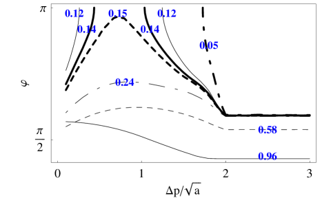
Figure 2: Curves in the $(\Delta p/\sqrt{a},\varphi)$ space on which $a(\omega\rightarrow 0^{-})=a(\omega\rightarrow 0^{+})$ labeled by the values of the initial magnetization $M_{0}$. The range of the angle $\varphi$ is restricted to the interval $[0;\pi]$.

Figure 2 represents the curves, in the $(\Delta p/\sqrt{a},\varphi)$ space, on which the time asymptotic magnetizations $a$ for $\omega=0^{-}$ and $\omega=0^{+}$ coincide, for several values of the initial magnetization $M_{0}$. Here the range of the angle $\varphi$ is restricted to the interval $[0;\pi]$. The full plot in the $[0;2\pi]$ range can be recovered by an axial symmetry about the horizontal line $\varphi=\pi$ (since when $\varphi$ is solution, then $2\pi-\varphi$ is also solution by switching the up and down waves in (7)). When $\Delta p/\sqrt{a}$ becomes larger than 2, $\varphi$ remains constant since resonance cat’s eye has been fully covered and that regular contributions (17) from the outer region cancel out.

Interestingly enough, when $M_{0}$ is sufficiently small (roughly below 0.15), there appears a gap, namely a region of the rescaled parameter $\Delta p/\sqrt{a}$, where the time asymptotic magnetizations for $\omega\equiv 0$ and $\omega=0^{+}$ do not intersect. This is reminiscent of the first order nature of the out-of-equilibrium phase transitions, associated with a discontinuity of the order parameter at the transition, evidenced in some already mentioned previous numerical works [10] and thermodynamical analysis [11], for the same domain of $M_{0}$. It is interesting to note here that the analysis by itself is able to unveil that the presumed continuity between Eqs. (6)-(7) cannot be satisfied in that domain, since $a$ is not continuous.

6 Derivation of the time-asymptotic state: a proof of principle

In order to fully characterize the transition, namely, for a given $M_{0}$, determine the time-asymptotic values of the magnetization $a$, of the wave phase $\varphi$ and determine the transition energy through $\Delta p$, an extra condition is needed. The natural additional relation to fulfill is given by the continuity of the energy at the transition. Its expression is $h[f]\equiv K[f]+1/2\left[1-\left(M[f]\right)^{2}\right]$, with the kinetic energy $K[f]=\int\int p^{2}/2f\left(p,\theta,t\right)dpd\theta$. In the regular domain, namely for the case $\omega\rightarrow 0^{-}$ with $h_{1}(p,\theta)=h_{1}\left(p_{0},\theta_{0}\right)=p^{2}/2-a\cos\left(\theta-\varphi\right)$, neglecting the effect of transient and using Liouville theorem, the time average of the kinetic energy is given by

$$\left\langle K[f]\right\rangle_{t}^{\omega\rightarrow 0^{-}} = \frac{1}{4\Delta p\Delta\theta}\int\limits_{-\Delta p}^{+\Delta p}dp_{0}\int\limits_{-\Delta\theta}^{\Delta\theta}d\theta_{0}h_{1}\left(p_{0},\theta_{0}\right)+\frac{a}{4\Delta p\Delta\theta}\int\limits_{-\Delta p}^{+\Delta p}dp_{0}\int\limits_{-\Delta\theta}^{\Delta\theta}d\theta_{0}\left\langle\cos\left(\theta-\varphi\right)\right\rangle_{t}$$ (19)

$$= \frac{1}{2\Delta p}\int\limits_{-\Delta p}^{+\Delta p}dp_{0}\frac{p_{0}^{2}}{2}-\frac{a}{2\Delta\theta}\int\limits_{-\Delta\theta}^{\Delta\theta}d\theta_{0}\cos\left(\theta_{0}-\varphi\right)+a^{2},$$

where the identity (13) was used. The continuity of the energy at the phase transition amounts then to the identity

$$\frac{\Delta p^{2}}{6}-aM_{0}\cos\varphi+a^{2}-\left\langle K[f]\right\rangle_{t}^{\omega\rightarrow 0^{+}}=\frac{1}{2}\left(\left\langle M[f]^{2}\right\rangle_{t}^{\omega\rightarrow 0^{-}}-\left\langle M[f]^{2}\right\rangle_{t}^{\omega\rightarrow 0^{+}}\right),$$ (20)

where time averages may be computed using the exact characteristics for $h_{1}$ in the $\omega\rightarrow 0^{-}$ case and the numerically obtained ones in the $\omega\rightarrow 0^{+}$ case.

This procedure would amount to determine the transition as an initial value problem, a truly desirable perspective that would involve the knowledge of the sole one-particle Vlasov dynamics without any reference to equilibrium statistical mechanics. Yet this desirable perspective is out of reach of the present analysis, surely due to the presently too stringent condition on the decay of the transient force field. The obtained values of the transition energies [12] are actually sensibly below the numerically [8] or thermodynamically computed ones [11]. This discrepancy can be already inferred from Fig. 3. This Figure displays the possible time-asymptotic values of the magnetization $a$ at the phase transition in the case where $a(\omega\rightarrow 0^{-})$ and $a(\omega\rightarrow 0^{+})$ coincide. As in Fig. 2, it is clear that, for low enough $M_{0}$, there exists some forbidden range for $\Delta p$ that may signal a discontinuity of the order parameter associated to the first order transition region. It is also clear from this picture, that, at least for low enough $M_{0}$, the possible $\Delta p$ are bounded by values ($\simeq 1$) which would yield values of the energy transition $U_{c}(M_{0})$ below the available numerically computed [10] and thermodynamically predicted ones [11].

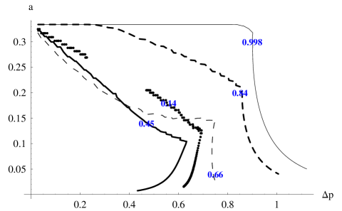
Figure 3: Curves in the $(\Delta p,a)$ space on which $a(\omega\rightarrow 0^{-})=a(\omega\rightarrow 0^{+})$ labeled by the values of the initial magnetization $M_{0}$.

Finally, in the domain of initial magnetizations where the out-of-equilibrium phase transitions are of first order, the additional identity (20) is insufficient to close the system of time-asymptotic parameters because $a$ is not continuous at the transition. This signals that the continuity assumption made in Eqs. (6) and (7) breaks: $\omega(U,M_{0})$ is strictly positive in the upper critical domain and its knowledge at the ”right side” of transition line is required.

7 Conclusion

To the author’s knowledge, this study is the first to address the issue of out-of-equilibrium phase transitions in the HMF model from the perspective of an initial value problem in the Vlasov limit. The essential point of this Letter is to propose a picture unveiling the nature of the phase transition: This corresponds to a brutal open-up of the time-asymptotic Vlasov one-particle phase space. The phase transition coincides with a jump between a time-asymptotic phase space foliated by energy lines and a phase space divided between an ergodic and a regular [21] components. It is proposed as a mechanism for second order phase transitions compatible with non-vanishing time-asymptotic values of the order parameter in mean-field long-range systems. As a byproduct, this study shows indirectly that the a priori reasonable hypothesis of a rapid decay of the time-asymptotic transient force field may not be satisfied by the HMF model. This is a posteriori not astonishing in view of the numerous recent papers reporting incomplete relaxation and deficient mixing properties in such a long-range system [22, 23, 24, 25, 26]. It remains to elucidate whether relaxing the hypothesis on the transient field would still be compatible with a purely dynamical initial value treatment, e.g. in the spirit of Lancellotti and Dorning’s approach. The present approach underlines the importance of the knowledge of the time-asymptotic spectrum $\omega(U,M_{0})$ of the dynamics. It would be instructive to proceed to time-Fourier transforms of large time Vlasov numerical simulations in order to extract this information.

Very recently, the author became aware of the just published paper by Leoncini et al. [27] whose possible connections with the present approach would be interesting to explore.

- [1] \NameAntoni M. Ruffo S. \REVIEWPhys. Rev. E 5219952361.
- [2] \NameElskens Y. Antoni M. \REVIEWPhys. Rev. E5519976575.
- [3] \NameBarré J., Bouchet F., Dauxois T., Ruffo S. \REVIEWEur. Phys. J. B292002577.
- [4] \NameLeyvraz F., Firpo M.-C., Ruffo S. \REVIEWJ. Phys. A3520024413.
- [5] \NameTsallis C. \REVIEWBrazil. J. Phys.2919991.
- [6] \NameFirpo M.-C., Doveil F., Elskens Y., Bertrand P., Poleni M. Guyomarc’h D. \REVIEWPhys. Rev. E642001026407.
- [7] \NamePluchino A., Rapisarda A. Tsallis C. \REVIEWEPL80200726002.
- [8] \NameBachelard R., Chandre C., Fanelli D., Leoncini X., Ruffo S. \REVIEWPhys. Rev. Lett.1012008260603.
- [9] \NameAntoniazzi A., Califano F., Fanelli D. Ruffo S. \REVIEWPhys. Rev. Lett.982007150602.
- [10] \NameAntoniazzi A., Fanelli D., Ruffo S. Yamaguchi Y.Y. \REVIEWPhys. Rev. Lett.992007040601.
- [11] \NameChavanis P.H. \REVIEWEur. Phys. J. B532006487.
- [12] \NameFirpo M.-C. unpublished.
- [13] \NameDemeio L. Holloway J.P. \REVIEWJ. Plasma Physics46199163.
- [14] It cannot, also, be definitely ruled out, on the basis of recent finite- numerical simulations [8], that the proposed time-asymptotic picture, as depicted in Fig. 1, be embedded in additional periodicities, such as a time-asymptotic periodic behavior of the magnetization. Vlasov simulations, in the line of Ref. [9], would be required to ascertain this by discarding finite- effects. This would not, however, change the phase transition description that considers only the time average limit.
- [15] \NameLancellotti C. Dorning J.J. \REVIEWPhys. Rev. Lett. 8119985137.
- [16] \NameLancellotti C. Dorning J.J. \REVIEWPhys. Rev. E 682003 026406.
- [17] \NameLichtenberg A.J. Lieberman M.A. \BookRegular and Stochastic Motion \PublSpringer-Verlag, New York \Year1983.
- [18] \NameMenyuk C.R. \REVIEWPhys. Rev. A 3119853282.
- [19] \NameElskens Y. Escande D.F. \REVIEWPhysica D62199366.
- [20] \NameMirbach B. Casati G. \REVIEWPhys. Rev. Lett.8319991327.
- [21] Integrability here is relative to the time-asymptotic limit. This does not prevent the dynamics in the low energy domain to exhibit some ergodic properties through the transient field and does not invalidate statistical mechanics.
- [22] \NameTamarit F.A., Maglione G., Stariolo D.A. Anteneodo C. \REVIEWPhys. Rev. E712005036148.
- [23] \NameJain K., Bouchet F. Mukamel D. \REVIEWJ. Stat. Mech.2007P11008.
- [24] \NameYamaguchi Y.Y., Bouchet F. Dauxois T. \REVIEWJ. Stat. Mech.2007P01020.
- [25] \NameCampa A., Chavanis P.H., Giansanti A., Morelli G. \REVIEWPhys. Rev. E782008040102(R).
- [26] \NameFigueiredo A., Rocha Filho T.M. Amato M.A. \REVIEWEPL83200830011.
- [27] \NameLeoncini X., Van Den Berg T.L. and Fanelli D. \REVIEWEPL86200920002.