BPS invariants of $\mathcal{N}=4$ gauge theory on Hirzebruch surfaces

Abstract.

Generating functions of BPS invariants for $\mathcal{N}=4$ $U(r)$ gauge theory on a Hirzebruch surface with $r\leq 3$ are computed. The BPS invariants provide the Betti numbers of moduli spaces of semi-stable sheaves. The generating functions for $r=2$ are expressed in terms of higher level Appell functions for a certain polarization of the surface. The level corresponds to the self-intersection of the base curve of the Hirzebruch surface. The non-holomorphic functions are determined, which added to the holomorphic generating functions provide functions which transform as a modular form.

1. Introduction

The study of supersymmetric spectra of field theories and supergravities is a major subject in theoretical physics and also mathematics. The BPS invariant counts the number of BPS states weighted by a sign. From a more mathematical perspective, the index corresponds to topological invariants (e.g. the Euler number or the Betti numbers) of a moduli space of objects (of an appropriate category) corresponding to the BPS states.

One of the seminal papers on BPS invariants of supersymmetric gauge theory on a Kähler surface is Ref. [34] by Vafa and Witten. They show that the topologically twisted path integral localizes on the instanton solutions, and equals the generating function of the Euler numbers of instanton moduli spaces, whose natural compactification is the moduli space of semi-stable sheaves. One of their main motivations was to test the strong-weak coupling duality [30] or $S$-duality, which acts by $SL(2,\mathbb{Z})$ transformations on the theory. The coupling constant $g$ and the theta angle $\theta$ combine to the modular parameter $\tau=\frac{\theta}{2\pi}+\frac{4\pi i}{g^{2}}$. $S$-duality suggests that the generating function of the BPS invariants (3.2) should exhibit modular properties if the gauge group is $SU(r)$ or $U(r)$. They tested this in various cases, for example for sheaves with rank $r=1$ [12], and $r=2$ on $\mathbb{P}^{2}$ [36, 37, 19]. The generating functions for rank 1 were found to be genuine (weakly) holomorphic modular forms. However the generating functions for rank 2 transform only approximately as a modular form. These functions are (mixed) mock modular forms, i.e. functions which do transform as a modular form only after the addition of a non-holomorphic “completion” [41].

Ref. [34] has inspired many results in later years. In particular, for $r=2$ the dependence of the BPS invariant on the polarization $J\in H^{2}(S,\mathbb{Z})$ was included in the generating functions using indefinite theta functions [14]. Moreover, the reduced modular properties for $r\geq 2$ were understood physically as a “holomorphic anomaly” [29, 1].

Although modularity has proven useful for various computations [29, 39, 14], physical expectations for $r>2$ could never be rigorously tested since generating functions for $r>2$ were not known. This was one of the motivations for [27], which computed the generating functions of refined BPS invariants for $r=3$ on $\mathbb{P}^{2}$ and its blow-up $\tilde{\mathbb{P}}^{2}$, which is the Hirzebruch surface $\Sigma_{1}$. A convenient property of $\Sigma_{1}$ is that the BPS invariants vanish for certain choices of the first Chern class and choice of polarization. Wall-crossing and the blow-up formula [38] provide then the invariants in the other chambers and for $\mathbb{P}^{2}$.

This article generalizes the computation of the generating function $\mathcal{Z}_{r}(z,\rho,\tau;\Sigma_{1},J)$ of BPS invariants for $r\leq 3$ of Ref. [27] to more general Hirzebruch surfaces $\Sigma_{\ell}$, where $-\ell$ is the self-intersection number of the base curve of $\Sigma_{\ell}$. The arguments $z\in\mathbb{C}$, $\rho\in H^{2}(\Sigma_{\ell},\mathbb{C})$ and $\tau\in\mathcal{H}$ in $\mathcal{Z}_{r}(z,\rho,\tau;\Sigma_{\ell},J)$ are generating variables for the Betti numbers of the moduli spaces, and first & second Chern classes of the sheaves respectively.

Section 3.1 derives expressions for the generating functions with $r=2$ in terms of indefinite theta functions [14] and Appell functions of level $\ell$ [3, 32]. The non-holomorphic but modular completed functions $\widehat{\mathcal{Z}}_{2}(z,\rho,\tau;\Sigma_{\ell},J)$ are determined for $z\in\mathbb{C}$ (generating function of Betti numbers) as well as $z=\textstyle{\frac{1}{2}}$ (Euler numbers). Due to the presence of these terms the action of the heat operator $D_{r}$ on the generating function $\widehat{\mathcal{Z}}_{r}(\rho,\tau;\Sigma_{\ell},J)$ (3) of Euler numbers does not vanish, which is known in the physics literature as a “holomorphic anomaly”. A novel result of the paper is that $D_{2}\widehat{\mathcal{Z}}_{2}(\rho,\tau;\Sigma_{\ell},J)$ in general consists of two terms (3.2):

(1.1) $$D_{2}\widehat{\mathcal{Z}}_{2}(\rho,\tau;\Sigma_{\ell},J)=C_{2}(\mathrm{Im}\,\tau,J)\,\mathcal{Z}_{1}(\rho,\tau,\Sigma_{\ell})^{2}+R_{2}(\rho,\tau;\Sigma_{\ell},J),$$

where $C_{2}(\mathrm{Im}\,\tau,J)$ is a simple function of $\mathrm{Im}\,\tau$ and $J$. The appearance of $\mathcal{Z}_{1}(\rho,z,\tau,\Sigma_{\ell})^{2}$ has been conjectured and discussed in the literature before [34, 29, 4], but the additional term $R_{2}(\rho,z,\tau;\Sigma_{\ell},J)$ is novel. Remarkably, the additional term vanishes for special choices of $J$, in particular for $J=-K_{\ell}$ where $K_{\ell}$ is the canonical class of $\Sigma_{\ell}$.

Another important property of the non-holomorphic completion is that it renders $\mathcal{Z}_{r}(\rho,z,\tau;\Sigma_{\ell},J)$ continuous as a function of the polarization $J$ [25], which is expected of a physical path integral. Although a more intrinsic derivation of the anomaly in physics or algebraic geometry is desirable, this gives already important insights.

Section 3.3 presents the holomorphic generating function for $r=3$ (3.3) for $r=3$ and presents the Tables 1-3 with the Betti numbers for $\ell=1$. The modular properties of $\mathcal{Z}_{3}(\rho,z,\tau;\Sigma_{\ell},J)$ are much more intricate then for $r=2$, and will be discussed elsewhere [5].

The outline of the paper is as follows. Section 2 reviews the necessary properties of sheaves and Hirzebruch surfaces, including BPS invariants and their wall-crossing. Section 3 defines the generating functions and gives explicit expressions for $r=1,2$ and 3. The non-holomorphic terms and the holomorphic anomaly are determined for $r=2$ in Subsection 3.2, and for $r=3$ Tables with Betti numbers are presented in 3.3.

2. Sheaves on Hirzebruch surfaces

The Gieseker-Maruyama moduli space of semi-stable sheaves with rank $r$ on $S$ is the natural compactification of the moduli space of instantons with gauge group $U(r)$, i.e. anti-self-dual solutions for the field strength: $*F=-F$. The Chern classes of the sheaf are determined by the topological classes of the instanton:

$$c_{1}=\frac{i}{2\pi}\mathrm{Tr}\,F,\qquad c_{2}-\frac{1}{2}c_{1}^{2}=\frac{1}{8\pi^{2}}\mathrm{Tr}\,F\wedge F.$$

Most of the following is phrased in the more algebraic language of sheaves, since this setting is most suitable for explicit computations.

2.1. Sheaves and stability

The Chern character of a sheaf $F$ on a surface $S$ is given by ch$(F)=r(F)+c_{1}(F)+\frac{1}{2}c_{1}(F)^{2}-c_{2}(F)$ in terms of the rank $r(F)$ and its Chern classes $c_{1}(F)$ and $c_{2}(F)$. The vector $\Gamma(F):=(r(F),\mathrm{ch}_{1}(F),\mathrm{ch}_{2}(F))$ summarizes the topological properties of $F$. Other frequently occuring quantities are the determinant $\Delta(F)=\frac{1}{r(F)}(c_{2}(F)-\frac{r(F)-1}{2r(F)}c_{1}(F)^{2})$, and $\mu(F)=c_{1}(F)/r(F)$.

Let $0\subset F_{1}\subset F_{2}\subset\dots\subset F_{s}=F$ be a filtration of the sheaf $F$. The quotients are denoted by $E_{i}=F_{i}/F_{i-1}$ with $\Gamma_{i}=\Gamma(E_{i})$. With the above notation, the discriminant $\Delta(F)$ is given in terms of the topological quantities of $E_{i}$ and $F_{i}$ by

(2.1) $$\Delta(F)=\sum_{i=1}^{s}\frac{r(E_{i})}{r(F)}\Delta(E_{i})-\frac{1}{2r(F)}\sum_{i=2}^{s}\frac{r(F_{i-1})\,r(F_{i})}{r(E_{i})}\left(\mu(F_{i-1})-\mu(F_{i})\right)^{2}.$$

The notion of a moduli space for sheaves is only well defined after the introduction of a stability condition. To this end let $C(S)\in H^{2}(S,\mathbb{Z})$ be the ample cone of $S$. Given a choice $J\in C(S)$, a sheaf $F$ is called $\mu$-stable if for every subsheaf $F^{\prime}\subset F$, $\mu(F^{\prime})\cdot J<\mu(F)\cdot J$, and $\mu$-semi-stable if $\mu(F^{\prime})\cdot J\leq\mu(F)\cdot J$. A wall of marginal stability $W$ is a (codimension 1) subspace of $C(S)$, such that $(\mu(F^{\prime})-\mu(F))\cdot J=0$, but $(\mu(F^{\prime})-\mu(F))\cdot J\neq 0$ away from $W$.

Let $S$ be a Kähler surface, whose intersection pairing on $H^{2}(S,\mathbb{Z})$ has signature $(1,b_{2}-1)$. Since at a wall, $(\mu_{2}-\mu_{1})\cdot J=0$ and $J^{2}>0$, we have $(\mu_{2}-\mu_{1})^{2}<0$. Therefore, the set of semi-stable filtrations for $F$, with $\Delta_{i}\geq 0$ is finite. The ample class $J$ provides natural projections $\mathbf{c}_{\pm}$ for an element $\mathbf{c}\in H^{2}(S,\mathbb{Z})$ to the positive and negative definite subspaces of $H^{2}(S,\mathbb{R})$:

(2.2) $$\mathbf{c}_{+}=\frac{\mathbf{c}\cdot J\,J}{J^{2}},\qquad\mathbf{c}_{-}=\mathbf{c}-\mathbf{c}_{+}.$$

2.2. Some properties of ruled surfaces

A ruled surface is a surface $\Sigma$ together with a surjective morphism $\pi:\Sigma\to C$ to a curve $C$, such that the fibre $\Sigma_{y}$ is isomorphic to $\mathbb{P}^{1}$ for every point $y\in C$. Let $f$ be the fibre of $\pi$, then $H_{2}(\Sigma,\mathbb{Z})=\mathbb{Z}C\oplus\mathbb{Z}f$, with intersection numbers $C^{2}=-\ell<0$, $f^{2}=0$ and $C\cdot f=1$. The canonical class is $K_{\Sigma}=-2C+(2g-2-\ell)f$. The holomorphic Euler characteristic $\chi(\mathcal{O}_{\Sigma})$ is for a ruled surface $1-g$. An ample class is parametrized by $J_{m,n}=m(C+\ell f)+nf\in C(\Sigma)$ with $m,n>0$. The following only considers surfaces with $g=0$, these are known as rationally ruled surfaces or Hirzebruch surfaces. They are denoted by $\Sigma_{\ell}$ and furthermore $K_{\ell}$ denotes the canonical class.

To learn about the set of semi-stable sheaves on $\Sigma_{\ell}$ for $J\in C(S)$, it is useful to first consider the restriction of the sheaves on $\Sigma_{\ell}$ to $f$. Namely the restriction to $E_{|f}$ is stable if and only if $E$ is $\mu$-stable for $J=J_{0,1}$ and in the adjacent chamber [15]. However, since every bundle of rank $\geq 2$ on $\mathbb{P}^{1}$ is a sum of line bundles, there are no stable bundles with $r\geq 2$ on $\mathbb{P}^{1}$. Therefore, the BPS invariant $\Omega(\Gamma,w;J)$ (defined in the next subsection) vanishes for $\Gamma=(r(F),-C-\alpha f,\mathrm{ch}_{2})$ with $r(F)\geq 2$ and $\alpha=0,1$.

2.3. Invariants and wall-crossing

The moduli space $\mathcal{M}_{J}(\Gamma)$ of semi-stable sheaves (with respect to the ample class $J$) whose rank and Chern classes are determined by $\Gamma$ has complex dimension:

(2.3) $$\dim_{\mathbb{C}}\mathcal{M}_{J}(\Gamma)=2r^{2}\Delta-r^{2}\chi(\mathcal{O}_{S})+1.$$

To define the refined BPS invariants $\Omega(\Gamma,w;J)$ in an informal way, let $p(X,s)=\sum_{i=0}^{2\dim_{\mathbb{C}}(X)}b_{i}s^{i}$, with $b_{i}$ the Betti numbers $b_{i}=\dim H^{2}(X,\mathbb{Z})$, be the Poincaré polynomial of a compact complex manifold $X$. Then:

(2.4) $$\Omega(\Gamma,w;J):=\frac{w^{-\dim_{\mathbb{C}}\mathcal{M}_{J}(\Gamma)}}{w-w^{-1}}\,p(\mathcal{M}_{J}(\Gamma),w).$$

The rational refined invariants are defined by [27]:

$$\bar{\Omega}(\Gamma,w;J)=\sum_{m|\Gamma}\frac{\Omega(\Gamma/m,-(-w)^{m};J)}{m}.$$

See [28] for a physical motivation of these rational invariants and [20, 31] for mathematical motivations. The numerical BPS invariant $\Omega(\Gamma;J)$ follows from the $\Omega(\Gamma,w;J)$ by:

(2.5) $$\Omega(\Gamma;J)=\lim_{w\to-1}(w-w^{-1})\,\Omega(\Gamma,w;J),$$

and similarly for the rational invariants $\bar{\Omega}(\Gamma;J)$.

A crucial tool for the computation of the generating functions in Section 3 is the wall-crossing formula, which provides the change $\Delta\Omega(\Gamma;J_{\mathcal{C}}\to J_{\mathcal{C}^{\prime}})$ across walls of marginal stability. Ref. [37] gives as criterion for his wall-crossing formula for $r=2$ that $K_{\ell}\cdot J<0$, which holds for any $\ell$ and $J\in C(\Sigma_{\ell})$. For $r=3$ more complicated wall-crossings appear, in particular walls where the slope of three rank 1 sheaves with different $c_{1}$ become equal. Physical arguments suggest that for these walls one could use the wall-crossing formulas of Kontsevich-Soibelman [20] or Joyce-Song [17] since they are shown to hold in both supergravity and field theory [6, 2, 11]. These wall-crossing formulas are derived for Donaldson-Thomas invariants, which are defined for 6-dimensional gauge theory on a Calabi-Yau 3-fold [9]. The mathematical justification for the use of these wall-crossing formulas for sheaves on surfaces is therefore not well established. Ref. [16] gives as criterion for the applicablity that $K_{S}^{-1}$ must be numerically effective (i.e. $-K_{S}\cdot D\geq 0$ for any curve in $D\in H^{2}(S,\mathbb{Z})$). This would exclude the Hirzebruch surfaces with $\ell>2$. The generating function (3.3) for $r=3$ is consistent with the wall-crossing formulas for DT-invariants and in agreement with previous results in the literature for $\ell=1$, but in view of the above requires at least for $\ell>2$ further justification.

Keeping in mind these comments, I continue by giving the explicit change of the invariants in case of primitive wall-crossing. To this end, define the following quantities:

$$\left<\Gamma_{1},\Gamma_{2}\right>=r_{1}r_{2}(\mu_{2}-\mu_{1})\cdot K_{S},\qquad\mathcal{I}(\Gamma_{1},\Gamma_{2};J)=r_{1}r_{2}(\mu_{2}-\mu_{1})\cdot J.$$

The change $\Delta\Omega(\Gamma_{1}+\Gamma_{2},w;J_{\mathcal{C}}\to J_{\mathcal{C}^{\prime}})$ for $\Gamma_{1}$ and $\Gamma_{2}$ primitive is [38, 20]

$$\Delta\Omega(\Gamma,w;J_{\mathcal{C}}\to J_{\mathcal{C}^{\prime}}) = -\textstyle{\frac{1}{2}}\left(\mathrm{sgn}(\mathcal{I}(\Gamma_{1},\Gamma_{2};J_{\mathcal{C}^{\prime}}))-\mathrm{sgn}(\mathcal{I}(\Gamma_{1},\Gamma_{2};J_{\mathcal{C}}))\right)$$

$$\times\left(w^{\left<\Gamma_{1},\Gamma_{2}\right>}-w^{-\left<\Gamma_{1},\Gamma_{2}\right>}\right)\Omega(\Gamma_{1},w;J)\,\Omega(\Gamma_{2},w;J).$$

with

$$\mathrm{sgn}(x)=\left\{\begin{array}[]{cl}1,&x>0,\\ 0,&x=0,\\ -1,&x<0.\end{array}\right.$$

The subscript ${W_{\mathcal{C}}}$ in $J_{W_{\mathcal{C}}}$ refers to a point in $\mathcal{C}$ which is sufficiently close to the wall $W$, such that no wall is crossed for the constituent between the wall and $J_{W_{\mathcal{C}}}$. Note that the wall is independent of $c_{2}$.

For the computation of the invariants of rank 3, one also needs to determine the wall-crossing formula across walls of marginal stability for non-primitive charges $2\Gamma_{1}+\Gamma_{2}$ and walls where the slope of three non-parallel charges becomes equal. These can be determined using the wall-crossing formulas [20, 17]. The result takes a simple form in terms of rational invariants and (2.3) [26].

3. Generating functions

This section computes the generating functions of the BPS invariants $\Omega(\Gamma,w;J)$. We start by defining the generating functions and a brief discussion of their properties. The generating function $\mathcal{Z}_{r}(\rho,z,\tau;S,J)$ for a Kähler surface $S$ is defined by:

$$\mathcal{Z}_{r}(\rho,z,\tau;S,J) = \sum_{c_{1},c_{2}}\,\bar{\Omega}(\Gamma,w;J)\,(-1)^{rc_{1}\cdot K_{S}}\,$$

$$\times\bar{q}^{r\Delta(\Gamma)-\frac{r\chi(S)}{24}-\frac{1}{2r}(c_{1}+rK_{S}/2)^{2}_{-}}q^{\frac{1}{2r}(c_{1}+rK_{S}/2)^{2}_{+}}e^{2\pi i\rho\cdot(c_{1}+rK_{S}/2)},$$

with $\rho\in H^{2}(S,\mathbb{C})$, $w=e^{2\pi iz}$ and $q=e^{2\pi i\tau}$. Twisting by a line bundle leads to an isomorphism of moduli spaces. It is therefore sufficient to determine $\Omega(\Gamma,w;J)$ only for $c_{1}\mod r$, and it moreover implies that $\mathcal{Z}_{r}(\rho,z,\tau;S,J)$ allows a theta function decomposition:

(3.1) $$\mathcal{Z}_{r}(\rho,z,\tau;S,J)=\sum_{\mu\in\Lambda^{*}/\Lambda}\overline{h_{r,\mu}(z,\tau;S,J)}\,\Theta_{r,\mu}(\rho,\tau;S),$$

where the bar over $h_{r,\mu}(z,\tau;S,J)$ denotes complex conjugation, and $h_{r,\mu}(z,\tau;S,J)$ and $\Theta_{r,\mu}(\rho,\tau;S)$ are defined by:

(3.2) $$h_{r,\mu}(z,\tau;S,J) = \sum_{c_{2}}\bar{\Omega}(\Gamma,w;J)\,q^{r\Delta(\Gamma)-\frac{r\chi(S)}{24}},$$

$$\Theta_{r,\mu}(\rho,\tau;S)\,\,\,\,\, = \sum_{\mathbf{k}\in H^{2}(S,r\mathbb{Z})+rK_{S}/2+\mu}(-1)^{r\mathbf{k}\cdot K_{S}}q^{\mathbf{k}^{2}_{+}/2r}\bar{q}^{-\mathbf{k}^{2}_{-}/2r}e^{2\pi i\rho\cdot\mathbf{k}}.$$

Note that $\Theta_{r,\mu}(\rho,\tau;S)$ depends on $J$ through $\mathbf{k}_{\pm}$ and does not depend on $z$.

The generating function of the numerical invariants $\Omega(\Gamma;J)$ follows simply from Eq. (2.5):

$$\mathcal{Z}_{r}(\rho,\tau;S,J)=\lim_{z\to\frac{1}{2}}\quad(w-w^{-1})\,\mathcal{Z}_{r}(z,\rho,\tau;S,J).$$

Physical arguments imply that this function transforms as a multivariable Jacobi form of weight $(\frac{1}{2},-\frac{3}{2})$ [34, 24] with a non-trivial multiplier system. For rank $>1$ this is only correct after the addition of a suitable non-holomorphic term [34, 29]. This is explained for $r=2$ in Subsections 3.1 and 3.2.

The functions $h_{r,c_{1}}(z,\tau)$ and $h_{r,c_{1}}(\tau)$ contain a factor which depends only on the rank $r$ and $b_{2}(S)$. It is therefore useful to define

$$f_{r,c_{1}}(z,\tau) = \left(\frac{i}{\theta_{1}(2z,\tau)\eta(\tau)^{b_{2}(S)-1}}\right)^{-r}h_{r,c_{1}}(z,\tau),$$

$$f_{r,c_{1}}(\tau) = \left(\frac{1}{\eta(\tau)^{\chi(S)}}\right)^{-r}h_{r,c_{1}}(\tau),$$

with $\theta_{1}(z,\tau)$ and $\eta(\tau)$ defined by (A). The function $f_{r,c_{1}}(\tau)$ follows from $f_{r,c_{1}}(z,\tau)$ by

(3.3) $$f_{r,c_{1}}(\tau)=\frac{(-1)^{r-1}}{2^{r-1}(r-1)!}\,\frac{1}{(2\pi i)^{r-1}}\partial_{z}^{r-1}f_{r,c_{1}}(z,\tau)|_{z=\frac{1}{2}}.$$

Note that the terms of degree $<r-1$ in the Taylor expansion with respect to $z$ of $f_{r,\mu}(z,\tau)$ vanish.

A useful relation is the “blow-up formula” which relates the generating function of a surface $S$ with that of its blow-up $\phi:\tilde{S}\to S$ at a non-singular point. Let $C_{1}$ be the exceptional divisor of $\phi$, and take $J\in C(S)$, $r$, and $c_{1}$ such that $\gcd(r,c_{1}\cdot J)=1$. The generating functions $h_{r,c_{1}}(z,\tau;S,J)$ and $h_{r,c_{1}}(z,\tau;\tilde{S},J)$ are then related by [36, 34, 38, 23, 14]:

(3.4) $$h_{r,\phi^{*}c_{1}-kC_{1}}(z,\tau;\tilde{S},J)=B_{r,k}(z,\tau)\,h_{r,c_{1}}(z,\tau;S,J),$$

with

$$B_{r,k}(z,\tau)=\frac{1}{\eta(\tau)^{r}}\sum_{\sum_{i=1}^{r}a_{i}=0\atop a_{i}\in\mathbb{Z}+\frac{k}{r}}q^{\frac{1}{2}\sum_{i=1}^{r}a_{i}^{2}}w^{\sum_{i<j}a_{i}-a_{j}}.$$

3.1. Rank 1 and 2

This subsection presents explicit expressions for $h_{r,c_{1}}(z,\tau;\Sigma_{\ell},J_{m,n})$. The result for $r=1$ and $S=\Sigma_{\ell}$ is simply [12]:

$$f_{1,c_{1}}(z,\tau;\Sigma_{\ell})=1.$$

Note that the dependence on $J$ could be omitted here since all rank 1 sheaves are stable. Moreover, there is also no dependence on $\ell$.

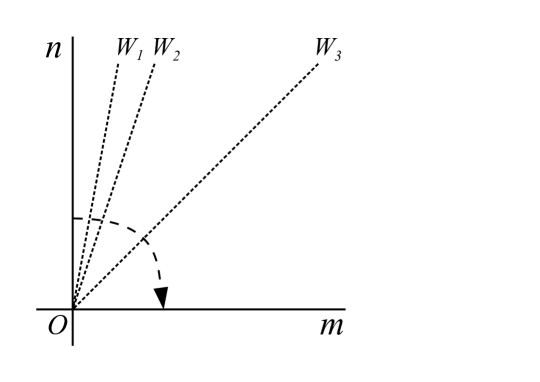
Figure 1. The ample cone of $\Sigma_{1}$, together with the three walls for $\Gamma=(2,-C-f,2)$, namely for $(a,b)=(1,0)$, $(2,0)$, $(3,0)$.

To compute the generating functions for $r\geq 2$, we use wall-crossing together with the fact that $\Omega(\Gamma,w;J_{0,1})=0$ for $c_{1}=-C+\alpha f$ and $r\geq 2$. In the following, $c_{1}(E_{2})$ is parametrised by $bC-af$. The walls are then at $\frac{m}{n}=\frac{2b-\beta}{2a-\alpha}$ for $r=2$, with $m,n\geq 0$. See Figure 1 for the walls for $\Delta(F)=\frac{9}{4}$, $r(F)=2$. One finds [14, 27] using Eq. (2.1):

$$f_{2,C-\alpha f}(z,\tau;\Sigma_{\ell},J_{m,n}) = -\textstyle{\frac{1}{2}}\sum_{a,b\in\mathbb{Z}}\textstyle{\frac{1}{2}}(\,\mathrm{sgn}((2b+1)n-(2a-\alpha)m)-\mathrm{sgn}(2b+1)\,)$$

$$\times\left(w^{(\ell-2)(2b+1)+2(2a-\alpha)}-w^{-(\ell-2)(2b+1)-2(2a-\alpha)}\right)$$

$$\times\,q^{\frac{\ell}{4}(2b+1)^{2}+\frac{1}{2}(2b+1)(2a-\alpha)}.$$

These functions are indefinite theta functions [13], which are sums over a subset of the positive definite sublattice of an indefinite lattice. Since the sum is only over a subset of the lattice, they transform as a modular form only after addition of a suitable non-holomorphic term (depending on $\bar{\tau}$ and $\bar{z}$) [41].

The computation of the invariants for $c_{1}=-\alpha f$ is much more involved since strictly semi-stable sheaves do exist for $J_{0,1}$ or if $\alpha=0$ for every $J\in C(\tilde{\mathbb{P}}^{2})$. We will circumvent this computation by determining the functions $f_{2,-\alpha f}(z,\tau;\Sigma_{\ell},J_{1,0})$ from modular transformations of $f_{2,C-\alpha f}(z,\tau;\Sigma_{\ell},J_{1,0})$. One can consequently determine the invariants for arbitrary $J_{m,n}$ by application of the wall-crossing formula.

We continue by writing $f_{2,C-\alpha f}(z,\tau;\Sigma_{\ell},J_{m,n})$ in terms of two new functions $A_{\ell,(\alpha,\beta)}(z,\tau)$ and $\vartheta_{\alpha,\beta}^{m,n}(z,\tau)$:

$$f_{2,\beta C-\alpha f}(z,\tau;\Sigma_{\ell},J_{m,n})=A_{\ell,(\alpha,\beta)}(z,\tau)+\vartheta_{\alpha,\beta}^{m,n}(z,\tau),\qquad\alpha,\beta\in\{0,1\}.$$

with

$$\vartheta_{\alpha,\beta}^{m,n}(z,\tau) = \sum_{a,b\in\mathbb{Z}}\textstyle{\frac{1}{2}}\left(\mathrm{sgn}(-(2a-\alpha))-\mathrm{sgn}((2b-\beta)n-(2a-\alpha)m)\right)$$

$$\times w^{(\ell-2)(2b-\beta)+2(2a-\alpha)}\,q^{\frac{\ell}{4}(2b-\beta)^{2}+\frac{1}{2}(2b-\beta)(2a-\alpha)}.$$

Then Eq. (3.1) gives for $A_{\ell,C-\alpha f}(z,\tau)$ for $\ell\geq 1$ after performing a geometric sum:

(3.6) $$A_{\ell,(1,1)}(z,\tau)=q^{\frac{\ell+2}{4}}w^{\ell}\sum_{n\in\mathbb{Z}}\frac{q^{\ell n(n+1)+n}w^{2(\ell-2)n}}{1-q^{2n+1}w^{4}},$$

$$A_{\ell,(0,1)}(z,\tau)\quad\,=-\frac{1}{2}\sum_{n\in\mathbb{Z}}q^{\frac{\ell}{4}(2n+1)^{2}}w^{(\ell-2)(2n+1)}+q^{\frac{\ell}{4}}w^{\ell-2}\sum_{n\in\mathbb{Z}}\frac{q^{\ell n(n+1)}w^{2(\ell-2)n}}{1-q^{2n+1}w^{4}}.$$

The functions in Eq. (3.6) are specializations of higher level Appell functions [3, 42], whose definition is recalled in Appendix A. These functions appeared earlier in mathematical physics in the theory of characters of superconformal algebras [10, 18, 32]. See [33] for a recent discussion. This might not be accidental since $\mathcal{N}=4$ Yang-Mills is well known to be related related to 2d conformal field theory by M-theory [29]. Deriving these functions explicitly from a 2-dimensional perspective is an interesting direction for future research.

Analogously to the indefinite theta functions, the Appell functions only transform as a modular (or Jacobi) form after addition of a non-holomorphic term. Eq. (A) gives the exact expression obtained by [42]. Application of this to our case of interest gives for the completion $\widehat{A}_{\ell,(\alpha,\beta=1)}(z,\tau)$ :

(3.7) $$\widehat{A}_{\ell,(\alpha,\beta)}(z,\tau) = A_{\ell,(\alpha,\beta)}(z,\tau)+\frac{1}{2}\sum_{k=0}^{\ell-1}\left(\sum_{n_{1}=2k+\beta\ell+\alpha\atop\mod 2\ell}w^{\frac{\ell-2}{\ell}n_{1}}q^{\frac{n_{1}^{2}}{4\ell}}\right)$$

$$\times\sum_{n_{2}=-2k-\alpha\atop\mod 2\ell}\left(\mathrm{sgn}(n_{2})-E\left(\left(n_{2}+2(\ell+2)\,\mathrm{Im}\,z/y\right)\sqrt{y/\ell}\right)\right)w^{-\frac{\ell+2}{\ell}n_{2}}q^{-\frac{n_{2}^{2}}{4\ell}},$$

with $y=\mathrm{Im}\,\tau$ and $E(x)=2\int_{0}^{x}e^{-\pi u^{2}}du$. The four functions $\widehat{A}_{\ell,(\alpha,\beta)}$ transform as a vector-valued Jacobi form of weight 1 and index $-8$ of $SL(2,\mathbb{Z})$ [32, 42]. One finds for the action of the generators $S$ and $T$ :

$$S: \quad\widehat{A}_{\ell,(\alpha,\beta)}\left(\frac{z}{\tau},\frac{-1}{\tau}\right)=\frac{\tau}{2}e^{2\pi i(-\frac{8\,z^{2}}{\tau})}\sum_{\tilde{\alpha},\tilde{\beta}\in\{0,1\}}(-1)^{\ell\beta\tilde{\beta}+\alpha\tilde{\beta}+\beta\tilde{\alpha}}\widehat{A}_{\ell,(\tilde{\alpha},\tilde{\beta})}(z,\tau),$$

$$T: \quad\widehat{A}_{\ell,(\alpha,\beta)}\left(z,\tau+1\right)\,=e^{2\pi i\frac{\beta^{2}+2\alpha\beta}{4}}\widehat{A}_{\ell,(\alpha,\beta)}\left(z,\tau\right)$$

The modular transformations (3.1) together with the single pole in $z$ of the refined invariants (2.4) do fix the functions $A_{\ell,(\alpha,0)}(z,\tau)$ to be:

$$A_{\ell,(1,0)}(z,\tau)=w^{2}\sum_{n\in\mathbb{Z}}\frac{q^{\ell n^{2}+n}w^{2(\ell-2)n}}{1-q^{2n}w^{4}}+\frac{i\,\eta(\tau)^{3}}{\theta_{1}(4z,\tau)},$$

$$A_{\ell,(0,0)}(z,\tau)\quad\,=-\frac{1}{2}\sum_{n\in\mathbb{Z}}q^{\ell n^{2}}w^{2(\ell-2)n}+\sum_{n\in\mathbb{Z}}\frac{q^{\ell n^{2}}w^{2(\ell-2)n}}{1-q^{2n}w^{4}}+\frac{i\,\eta(\tau)^{3}}{\theta_{1}(4z,\tau)}.$$

This agrees for $c_{1}=f$ with the generating function in Ref. [37] (Corollary 3.4). The completion of these functions is given by Eq. (3.7).

One can show the following relation between $A_{1,(\alpha,0)}(z,\tau)$ and $A_{1,(\alpha,1)}(z,\tau)$ using the quasi-periodicity formula (A.4):

(3.9) $$A_{1,(1,0)}(z,\tau)=\frac{\theta_{2}(2z,2\tau)}{\theta_{3}(2z,2\tau)}\,A_{1,(1,1)}(z,\tau),$$

$$A_{1,(0,0)}(z,\tau)\,\,\,\,=\frac{\theta_{3}(2z,2\tau)}{\theta_{2}(2z,2\tau)}\,A_{1,(0,1)}(z,\tau).$$

This relation is understood in algebraic geometry by the blow-up formula (3.4), which relates the functions $h_{2,c_{1}}(z,\tau;\Sigma_{1},J_{1,0})$ with $c_{1}=C-\alpha f$ to those with $c_{1}=-\alpha f$. For $h_{2,c_{1}}(z,\tau;\mathbb{P}^{2})$ one recovers the result of [4]. The multiplicative relation (3.9) does not hold for $\ell>1$, since $\Sigma_{\ell>1}$ is the blow-up of the weighted projective plane $(1,1,\ell)$ at its singular point [8], and the blow-up formula is thus not applicable.

What remains is to complete the indefinite theta functions $\vartheta_{\alpha,\beta}^{m,n}(z,\tau)$. One finds using Ref. [41]:

$$\widehat{\vartheta}_{\alpha,\beta}^{m,n}(z,\tau) = \sum_{a,b\in\mathbb{Z}}\textstyle{\frac{1}{2}}\left[E\left((-2a+\alpha+2(\ell+2)\mathrm{Im}z/y)\sqrt{y/\ell}\right)\right.$$

$$-\left.E\left(((2b-\beta)n-(2a-\alpha)m+2(2n+(\ell+2)m)\mathrm{Im}\,z/y)\sqrt{y/J^{2}_{m,n}}\right)\right]$$

$$\times w^{(\ell-2)(2b-\beta)+2(2a-\alpha)}\,q^{\frac{\ell}{4}(2b-\beta)^{2}+\frac{1}{2}(2b-\beta)(2a-\alpha)}$$

with $J_{m,n}^{2}=m(\ell m+2n)$. The completion for $f_{2,\beta C-\alpha f}$ follows directly from $\widehat{f}_{2,\beta C-\alpha f}=\widehat{A}_{\ell,(\alpha,\beta)}+\widehat{\vartheta}_{\alpha,\beta}^{m,n}$. The non-holomorphic term of the first line in Eq. (3.1) is cancelled by the non-holomorphic term of $\widehat{A}_{\ell,(\alpha,\beta)}(z,\tau)$. Thus for the completion of $f_{2,\beta C-\alpha f}$ (and therefore also of $h_{2,\beta C-\alpha f}$) the non-holomorphic part of the second line in Eq. (3.1) suffices. We define $\mathcal{\widehat{Z}}_{r}(\rho,z,\tau;S,J):=\sum_{\mu\in H^{2}(\Sigma_{\ell},\mathbb{Z}/r\mathbb{Z})}\overline{\widehat{h}_{r,\mu}(z,\tau;S,J)}\,\Theta_{r,\mu}(\rho,\tau;S)$.

3.2. Holomorphic anomaly for rank 2

This subsection derives $D_{r}\mathcal{\widehat{Z}}_{r}(\rho,\tau;\Sigma_{\ell},J)$ for $D_{r}=\partial_{\tau}+\frac{i}{4\pi r}\partial^{2}_{\rho_{+}}$ and $r=2$. Since $D_{r}\Theta_{r,\mu}(\rho,\tau;\Sigma_{\ell})=0$ for any $r$, it suffices to determine $\partial_{\bar{\tau}}\widehat{f}_{r,c_{1}}(\tau;\Sigma_{\ell},J)$. For a clear exposition, the generating functions are given in this subsection in terms of $K_{\ell}$, $J$ etc. instead of the explicit integers $\ell$, $m$ and $n$ etc.

We determine first the completion $\widehat{f}_{2,c_{1}}(\tau;\Sigma_{\ell},J)$ from the generating functions in the previous subsection. The result follows from the following three steps:

• use Eq. (3.3) after replacing the functions with their completions,

• use that $E(z)=2\int_{0}^{z}e^{-\pi u^{2}}du=\mathrm{sgn}(z)(1-\beta_{\frac{1}{2}}(z^{2}))$ with $z\in\mathbb{R}$ and

  $$\beta_{\nu}(x)=\int_{x}^{\infty}u^{-\nu}e^{-\pi u}du,$$

• and finally use

  $$\beta_{\frac{3}{2}}(x)=2x^{-\frac{1}{2}}e^{-\pi x}-2\pi\beta_{\frac{1}{2}}(x).$$

One obtains:

$$\widehat{f}_{2,c_{1}}(\tau;\Sigma_{\ell},J)=f_{2,c_{1}}(\tau;\Sigma_{\ell},J)+$$

$$\quad\sum_{\mathbf{c}\in-c_{1}\atop+H^{2}(\Sigma_{\ell},2\mathbb{Z})}\left(\frac{K_{\ell}\cdot J\,|\mathbf{c}\cdot J|}{8\pi J^{2}}\,\beta_{\frac{3}{2}}(\mathbf{c}_{+}^{2}\,y)-\frac{1}{4}K_{\ell}\cdot\mathbf{c}_{-}\,\mathrm{sgn}(\mathbf{c}\cdot J)\,\beta_{\frac{1}{2}}(\mathbf{c}_{+}^{2}\,y)\right)\,(-1)^{K_{\ell}\cdot\mathbf{c}}q^{-\mathbf{c}^{2}},$$

where $\mathbf{c}_{\pm}$ are given by Eq. (2.2). It is now straightforward to compute $\partial_{\bar{\tau}}\widehat{f}_{r,c_{1}}(\tau;\Sigma_{\ell},J)$:

$$\partial_{\bar{\tau}}\widehat{f}_{r,c_{1}}(\tau;\Sigma_{\ell},J) = \frac{i\,K_{\ell}\cdot J}{16\pi\,\sqrt{J^{2}}\,y^{\frac{3}{2}}}\,(-1)^{K_{\ell}\cdot c_{1}}\,\overline{\Theta_{2,-c_{1}-K_{\ell}}(0,\tau;\Sigma_{\ell})}$$

$$-\frac{i}{8\sqrt{y}}\sum_{\mathbf{c}\in-c_{1}\atop+H^{2}(\Sigma_{\ell},2\mathbb{Z})}K_{\ell}\cdot\mathbf{c}_{-}\,\frac{\mathbf{c}\cdot J}{\sqrt{J^{2}}}\,\,(-1)^{K_{\ell}\cdot\mathbf{c}}\,q^{-\mathbf{c}_{-}^{2}/4}\bar{q}^{\mathbf{c}_{+}^{2}/4}.$$

After combining this result with $\Theta_{2,c_{1}}(\rho,\tau;\Sigma_{\ell})$ as in (3.1) and manipulation of the lattice sums, one obtains for $D_{2}\mathcal{\widehat{Z}}_{2}(\rho,\tau;\Sigma_{\ell},J)$:

$$D_{2}\mathcal{\widehat{Z}}_{2}(\rho,\tau;\Sigma_{\ell},J) = \frac{-i\,K_{\ell}\cdot J}{16\pi\,\sqrt{J^{2}}\,y^{\frac{3}{2}}}\,\mathcal{Z}_{1}(\rho,\tau;\Sigma_{\ell},J)^{2}$$

$$+\frac{i}{8\sqrt{y}}\,\overline{h_{1,0}(\tau;\Sigma_{\ell})}^{2}\,\sum_{c_{1}\in H^{2}(\Sigma_{\ell},\mathbb{Z}/2\mathbb{Z})}\Upsilon_{c_{1}}(\tau,\Sigma_{\ell})\,\Theta_{2,c_{1}}(\rho,\tau;\Sigma_{\ell}),$$

where

$$\Upsilon_{c_{1}}(\tau,\Sigma_{\ell})=\sum_{\mathbf{c}\in-c_{1}\atop+H^{2}(\Sigma_{\ell},2\mathbb{Z})}K_{\ell}\cdot\mathbf{c}_{-}\,\frac{\mathbf{c}\cdot J}{\sqrt{J^{2}}}\,\,(-1)^{K_{\ell}\cdot\mathbf{c}}\,q^{\mathbf{c}_{+}^{2}/4}\bar{q}^{-\mathbf{c}_{-}^{2}/4}.$$

Interestingly, Eq. (3.2) differs from the conjectured form of the anomaly [34, 29, 1]. The first line has the expected factorized form, which is attributed to reducible connections or polystable sheaves [34] or multiple M5-branes [29]. However, the novel second line does not factorize and is less easily interpreted. It does vanish for special values of $J$, in particular for $J=-K_{\ell}$ since then $K_{\ell}\cdot\mathbf{c}_{-}=0$. But for $\ell\geq 2$, $K_{\ell}$ lies outside $C(S)$ and is thus not a permissible choice for $J$. Viewing the surface as part of a local Calabi-Yau 3-fold geometry, $J=-K_{S}$ corresponds to the attractor point from the point of view of supergravity [25]. It is therefore rather interesting that $\mathcal{\widehat{Z}}(\rho,\tau;\Sigma_{\ell},J)$ simplifies at this point.

The function $\Upsilon_{c_{1}}(\tau,\Sigma_{\ell})$ vanishes also for $\ell=1$ and $J=C+f$ [4], which is not equal to $-K_{1}$. For this choice, the blow-up formula gives the generating function for $\mathbb{P}^{2}$, where $J=-K_{\mathbb{P}^{2}}$ is satisfied automatically. It is thus in agreement with these examples to conjecture that generically for a Kähler surface $S$, $D_{2}\mathcal{\widehat{Z}}_{2}(\rho,\tau;S,J)=\frac{-i\,\sqrt{K_{S}^{2}}}{16\pi\,y^{\frac{3}{2}}}\,\mathcal{Z}_{1}(\rho,\tau;S,-K_{s})^{2}$ if $K_{S}\in C(S)$. Of course, a more intrinsic explanation based on gauge theory or algebraic geometry is desirable.

3.3. Rank 3

This subsection presents the generating functions $h_{3,\beta C-\alpha f}(z,\tau;\Sigma_{\ell},J)$ with $\beta\neq 0\mod 3$. This condition on $\beta$ ensures that $h_{3,\beta C-\alpha f}(z,\tau;\Sigma_{\ell},J)=0$ for $J=J_{0,1}$ analogously to $r=2$. The computation of $h_{3,\beta C-\alpha f}(z,\tau;\Sigma_{\ell},J)$ therefore reduces again to application of the wall-crossing formula. This is for $r=3$ more complicated than for $r=2$ since:

• the functions $h_{2,c_{1}}(z,\tau;\Sigma_{\ell},J)$ do themselves depend on $J$, and need to be determined sufficiently close to the appropriate wall.

• the total charge $\Gamma$ can be of a sum of 3 charges $\sum_{i=1}^{3}\Gamma_{i}$ such that at a wall $W$ the slopes of these three constituents might be equal. This in particular happens for “semi-primitive wall-crossing” where $\Gamma(F)=2\Gamma_{1}+\Gamma_{2}$.

Nevertheless, the wall-crossing formulas [20, 17] imply a relatively simple form for the generating functions [26, 27]. One obtains for $\ell\geq 1$:

$$f_{3,\beta C-\alpha f}(z,\tau;\Sigma_{\ell},J_{m,n}) = -\sum_{a,b\in\mathbb{Z}}\textstyle{\frac{1}{2}}(\,\mathrm{sgn}((3b-2\beta)n-(3a-2\alpha)m)-\mathrm{sgn}(3b-2\beta)\,)$$

$$\times\left(w^{(\ell-2)(3b-2\beta)+2(3a-2\alpha)}-w^{-(\ell-2)(3b-2\beta)-2(3a-2\alpha)}\right)$$

$$\times\,q^{\frac{\ell}{12}(3b-2\beta)^{2}+\frac{1}{6}(3b-2\beta)(3a-2\alpha)}$$

$$\times\,f_{2,bC-af}(z,\tau;\Sigma_{\ell},J_{|3b-2\beta|,|3a-2\alpha|}),$$

for $\beta=1,2\mod 3$ and $\alpha\in\mathbb{Z}$. Writing out the lattice sums in Eq. (3.3), one finds a novel indefinite theta function. It has signature $(2,2)$ and the condition which determines whether or not a lattice point contributes depends quadratically on the lattice vector, whereas previously described indefinite theta functions have signature $(n,1)$ and the condition depends linearly on the lattice vector [13, 41]. A detailed discussion of the (mock) modular properties of $h_{3,c_{1}}(z,\tau;\Sigma_{\ell},J)$ will appear in a future article [5].

Tables 1-3 list Betti numbers for $c_{1}=-C-\alpha f$ with $\alpha=1,2,3$ and $\ell=1$, which are in agreement with the expected dimension (2.3). One can relate the Betti numbers for $c_{1}=-2C-\alpha f$ to these by using $h_{r,c_{1}}=h_{r,-c_{1}}$, and $h_{r,c_{1}+\mathbf{k}}=h_{r,c_{1}}$ for $\mathbf{k}\in H_{2}(S,r\mathbb{Z})$. With a little more work, one can verify that $h_{3,c_{1}}(z,\tau;\Sigma_{1},J_{1,0})$ satisfies the relations implied by the blow-up formula (3.4).

$c_{2}$	$b_{0}$	$b_{2}$	$b_{4}$	$b_{6}$	$b_{8}$	$b_{10}$	$b_{12}$	$b_{14}$	$b_{16}$	$b_{18}$	$b_{20}$	$b_{22}$	$b_{24}$	$\chi$
2	1	2	4	4										18
3	1	3	9	20	37	53	59							305
4	1	3	10	25	59	119	218	338	450	490				2936
5	1	3	10	26	64	141	294	562	997	1602	2301	2886	3117	20891

Table 1. The Betti numbers $b_{n}$ (with $n\leq\dim_{\mathbb{C}}\mathcal{M}$) and the Euler numbers $\chi$ of the moduli spaces of stable sheaves on $\Sigma_{1}$ with $r=3$, $c_{1}=-C$, and $2\leq c_{2}\leq 6$ for $J=(1,\varepsilon)$.

$c_{2}$	$b_{0}$	$b_{2}$	$b_{4}$	$b_{6}$	$b_{8}$	$b_{10}$	$b_{12}$	$b_{14}$	$b_{16}$	$b_{18}$	$b_{20}$	$b_{22}$	$b_{24}$	$b_{26}$	$\chi$
2	1	1													3
3	1	3	8	14	17										69
4	1	3	10	24	53	93	136	152							792
5	1	3	10	26	63	135	268	470	725	950	1043				6345
6	1	3	10	26	65	145	310	612	1144	1970	3113	4391	5462	5873	40377

Table 2. The Betti numbers $b_{n}$ (with $n\leq\dim_{\mathbb{C}}\mathcal{M}$) and the Euler numbers $\chi$ of the moduli spaces of stable sheaves on $\Sigma_{1}$ with $r=3$, $c_{1}=-C-f$, and $2\leq c_{2}\leq 6$.

$c_{2}$	$b_{0}$	$b_{2}$	$b_{4}$	$b_{6}$	$b_{8}$	$b_{10}$	$b_{12}$	$b_{14}$	$b_{16}$	$b_{18}$	$b_{20}$	$b_{22}$	$\chi$
3	1	2	3										9
4	1	3	9	19	31	36							162
5	1	3	10	25	58	113	192	264	297				1629
6	1	3	10	26	64	140	288	536	907	1348	1733	1885	11997

Table 3. The Betti numbers $b_{n}$ (with $n\leq\dim_{\mathbb{C}}\mathcal{M}$) and the Euler numbers $\chi$ of the moduli spaces of stable sheaves on $\Sigma_{1}$ with $r=3$, $c_{1}=-C-2f$, and $3\leq c_{2}\leq 6$.

Appendix A Modular functions

Define $q:=e^{2\pi i\tau}$, $w:=e^{2\pi iz}$, with $\tau\in\mathbb{H}$ and $z\in\mathbb{C}$. The Dedekind eta and Jacobi theta functions are defined by:

$$\eta(\tau)\quad\,\,:=q^{\frac{1}{24}}\prod_{n=1}^{\infty}(1-q^{n}),$$

(A.1) $$\theta_{1}(z,\tau):=i\sum_{r\in\mathbb{Z}+\frac{1}{2}}(-1)^{r-\frac{1}{2}}q^{\frac{r^{2}}{2}}w^{r},$$

$$\theta_{2}(z,\tau):=\sum_{r\in\mathbb{Z}+\frac{1}{2}}q^{r^{2}/2}w^{r},$$

$$\theta_{3}(z,\tau):=\sum_{n\in\mathbb{Z}}q^{n^{2}/2}w^{n}.$$

The Appell function at level $\ell$ is defined by:

(A.2) $$A_{\ell}(u,v,\tau)=a^{\ell/2}\sum_{n\in\mathbb{Z}}\frac{(-1)^{\ell n}q^{\ell n(n+1)/2}b^{n}}{1-aq^{n}},$$

with $a=e^{2\pi iu}$ and $b=e^{2\pi iv}$. In order to give the completion $\widehat{A}_{\ell}(u,v,\tau)$, define

$$R(u,\tau) = \sum_{r\in\mathbb{Z}+\frac{1}{2}}\left(\,\mathrm{sgn}(r)-E\left((r+\mathrm{Im}\,u/y)\sqrt{2y}\right)\,\right)$$

$$\times(-1)^{r-\frac{1}{2}}a^{-r}q^{-r^{2}/2},$$

with $E(x)=2\int_{0}^{x}e^{-\pi u^{2}}du$. The completion $\widehat{A}_{\ell}(u,v,\tau)$ is then given by [42]

$$\widehat{A}_{\ell}(u,v,\tau) = A_{\ell}(u,v,\tau)+\frac{i}{2}\sum_{k=0}^{\ell-1}\,a^{k}\,\theta_{1}(v+k\tau+(\ell-1)/2,\ell\tau)$$

$$\times R(\ell u-v-k\tau-(\ell-1)/2,\ell\tau),$$

and transforms as a multivariable Jacobi form of weight 1 and index $\frac{1}{2}\left(\begin{array}[]{cc}-\ell&1\\ 1&0\end{array}\right)$. The Appell function for $\ell=1$ is related to the Lerch-Appell function: $\mu(u,v,\tau)=A_{1}(u,v,\tau)/\theta_{1}(v)$, which satisfies the quasi-periodicity property [41]:

(A.4) $$\mu(u+z,v+z,\tau)-\mu(u,v,\tau)=\frac{\eta(\tau)^{3}\,\theta_{1}(u+v+z,\tau)\,\theta_{1}(z,\tau)}{\theta(u,\tau)\,\theta(v,\tau)\,\theta(u+z,\tau)\,\theta(v+z,\tau)},$$

for $u,v,u+z,v+z\notin\mathbb{Z}\tau+\mathbb{Z}$.

References

• [1] M. Alim, B. Haghighat, M. Hecht et al., Wall-crossing holomorphic anomaly and mock modularity of multiple M5-branes, [arXiv:1012.1608 [hep-th]].
• [2] E. Andriyash, F. Denef, D. L. Jafferis and G. W. Moore, Wall-crossing from supersymmetric galaxies, arXiv:1008.0030 [hep-th].
• [3] M. P. Appell, Sur les fonctions doublement périodique de troisième espèce, Annales scientifiques de l’E.N.S., (1886) 9-42.
• [4] K. Bringmann and J. Manschot, From sheaves on $\mathbb{P}^{2}$ to a generalization of the Rademacher expansion, American J. of Math. [arXiv:1006.0915 [math.NT]].
• [5] K. Bringmann, J. Manschot and S. P. Zwegers, In preparation.
• [6] F. Denef and G. W. Moore, Split states, entropy enigmas, holes and halos, [arXiv:hep-th/0702146].
• [7] T. Dimofte and S. Gukov, Refined, Motivic, and Quantum, Lett. Math. Phys.  91 (2010) 1 [arXiv:0904.1420 [hep-th]].
• [8] I. V. Dolgachev, Weighted Projective Varieties, in Group Actions and Vector Fields, Lecture Notes in Math. 956, Springer-Verlag (1982), 34-71.
• [9] S. K. Donaldson and R. P. Thomas, Gauge theory in higher dimensions in “The geometric universe: science, geometry and the work of Roger Penrose”, Oxford University Press (1998).
• [10] T. Eguchi, A. Taormina, On the unitary representations of N=2 and N=4 superconformal algebras, Phys. Lett.  B210, 125 (1988).
• [11] D. Gaiotto, G. W. Moore and A. Neitzke, Four-dimensional wall-crossing via three-dimensional field theory, arXiv:0807.4723 [hep-th].
• [12] L. Göttsche, The Betti numbers of the Hilbert scheme of points on a smooth projective surface, Math. Ann. 286 (1990) 193.
• [13] L. Göttsche, D. Zagier, Jacobi forms and the structure of Donaldson invariants for 4-manifolds with $b_{+}=1$, Selecta  Math., New Ser. 4 (1998) 69. [arXiv:alg-geom/9612020].
• [14] L. Göttsche, Theta functions and Hodge numbers of moduli spaces of sheaves on rational surfaces, Comm. Math. Physics  206 (1999) 105 [arXiv:math.AG/9808007].
• [15] D. Huybrechts and M. Lehn, “The geometry of moduli spaces of sheaves,” (1996).
• [16] D. Joyce, Configurations in Abelian categories. IV. Invariants and changing stability conditions., arXiv:math/0410268 [math.AG].
• [17] D. Joyce and Y. Song, A theory of generalized Donaldson-Thomas invariants, arXiv:0810.5645 [math.AG].
• [18] V. G. Kac and M. Wakimoto, Integrable highest weight modules over affine superalgebras and Appell’s function, Commun. Math. Phys. 215 (2000) 631-682.
• [19] A. Klyachko, Moduli of vector bundles and numbers of classes, Funct. Anal. and Appl. 25 (1991), 67–68.
• [20] M. Kontsevich and Y. Soibelman, Stability structures, motivic Donaldson-Thomas invariants and cluster transformations, [arXiv:0811.2435 [math.AG]].
• [21] M. Kontsevich, Y. Soibelman, Cohomological Hall algebra, exponential Hodge structures and motivic Donaldson-Thomas invariants, [arXiv:1006.2706 [math.AG]].
• [22] M. Kool, Euler charactertistics of moduli spaces of torsion free sheaves on toric surfaces, arXiv:0906.3393 [math.AG].
• [23] W.-P. Li and Z. Qin, On blowup formulae for the $S$-duality conjecture of Vafa and Witten, Invent. Math.  136 (1999) 451-482 [arXiv:math.AG/9808007].
• [24] J. Manschot, On the space of elliptic genera, Commun. Num. Theor. Phys.  2 (2008) 803-833. [arXiv:0805.4333 [hep-th]].
• [25] J. Manschot, Stability and duality in $\mathcal{N}=2$ supergravity, Commun. Math. Phys. 299 (2010) 651-676, arXiv:0906.1767 [hep-th].
• [26] J. Manschot, Wall-crossing of D4-branes using flow trees, Adv. in Theor. Math. Physics, arXiv:1003.1570 [hep-th].
• [27] J. Manschot, The Betti numbers of the moduli space of stable sheaves of rank 3 on $P^{2}$, Lett. Math. Phys.  98 (2011) 65 [arXiv:1009.1775 [math-ph]].
• [28] J. Manschot, B. Pioline and A. Sen, Wall Crossing from Boltzmann Black Hole Halos, JHEP 1107 (2011) 059 [arXiv:1011.1258 [hep-th]].
• [29] J. A. Minahan, D. Nemeschansky, C. Vafa and N. P. Warner, E-strings and $\mathcal{N}=4$ topological Yang-Mills theories, Nucl. Phys.  B 527 (1998) 581 [arXiv:hep-th/9802168].
• [30] C. Montonen and D. Olive, Magnetic monopoles as gauge particles?, Phys. Lett.  B 72 (1977) 117.
• [31] H. Nakajima and K. Yoshioka Instanton counting and Donaldson invariants, Sūgaku 59 (2007) 131-153
• [32] A. M. Semikhatov, A. Taormina, I. Y. Tipunin, Higher level Appell functions, modular transformations, and characters, [math/0311314 [math-qa]].
• [33] J. Troost, The non-compact elliptic genus: mock or modular, JHEP 1006 (2010) 104 [arXiv:1004.3649 [hep-th]].
• [34] C. Vafa and E. Witten, A strong coupling test of S duality, Nucl. Phys.  B 431 (1994) 3 [arXiv:hep-th/9408074].
• [35] T. Weist, Torus fixed points of moduli spaces of stable bundles of rank three, arXiv:0903.0732 [math. AG].
• [36] K. Yoshioka, The Betti numbers of the moduli space of stable sheaves of rank 2 on $\mathbb{P}^{2}$, J. reine. angew. Math. 453 (1994) 193–220.
• [37] K. Yoshioka, The Betti numbers of the moduli space of stable sheaves of rank 2 on a ruled surface, Math. Ann. 302 (1995) 519–540.
• [38] K. Yoshioka, The chamber structure of polarizations and the moduli of stable sheaves on a ruled surface, Int. J. of Math. 7 (1996) 411–431 [arXiv:alg-geom/9409008].
• [39] K. Yoshioka, Euler characteristics of SU(2) instanton moduli spaces on rational elliptic surfaces, Commun. Math. Phys.  205 (1999) 501 [arXiv:math/9805003].
• [40] D. Zagier, Nombres de classes et formes modulaires de poids 3/2, C.R.  Acad.  Sc.   Paris, 281 (1975) 883.
• [41] S. P. Zwegers, “Mock Theta Functions,” Dissertation, University of Utrecht (2002)
• [42] S. P. Zwegers, “Multivariable Appell functions,” (2010).