Soliton–antisoliton pair production in particle collisions

Abstract

We propose general semiclassical method for computing the probability of soliton–antisoliton pair production in particle collisions. The method is illustrated by explicit numerical calculations in $(1+1)$–dimensional scalar field model. We find that the probability of the process is suppressed by an exponentially small factor which is almost constant at high energies.

Ever since the discovery of topological solitons, a question remains Drukier ; solitons ; *solitons1 of whether soliton–antisoliton (SA) pair can be produced at sizable probability in collision of two quantum particles. This process, which involves a transition from perturbative two–particle state to a non–perturbative state containing SA pair, eludes treatment by any of the standard methods. A general expectation Drukier ; unitarity ; *unitarity1; *unitarity2 is that the probability of the process is exponentially suppressed in weak coupling regime,

$${\cal P}(E)\sim\mathrm{e}^{-F(E)/g^{2}}\;,$$ (1)

where $E$ is the total energy, $g\ll 1$ is the coupling constant. Indeed, crudely speaking, one can think of solitons as bound states of $N_{S}\sim 1/g^{2}$ particles Drukier . Then the suppression (1) is due to multiparticle production unitarity .

In this Letter we propose general semiclassical method for computing the leading suppression exponent $F(E)$ of the inclusive process “two particles $\to$ SA pair + particles.” As a by–product, we calculate the exponent $F_{N}(E)$ of the same process with $N$ initial particles. In our method the problem is deformed by introducing a small parameter $\delta\rho$ which turns the process of SA pair production into a well–known tunneling process. To the best of our knowledge, no method of this kind has ever been proposed before.

For definiteness we consider $(1+1)$–dimensional scalar field theory with action 

$$S[\phi]=\frac{1}{g^{2}}\int d^{2}x\left[-\frac{1}{2}\phi\,\Box\phi-V(\phi)\right]\;.$$ (2)

This model possesses topological solitons if the scalar potential $V(\phi)$ has a pair of degenerate minima $\phi_{-}$ and $\phi_{+}$, see the inset in Fig. 1, solid line. Soliton and antisoliton solutions interpolate between the minima; their profiles are shown in Fig. 2a.

An obstacle to the semiclassical description of SA pair production is related to the fact that soliton and antisoliton attract each other and annihilate classically into $N_{SA}\sim 1/g^{2}$ particles. Thus, there is no potential barrier separating SA pair from the particle sector and the process under study cannot be treated as potential tunneling.

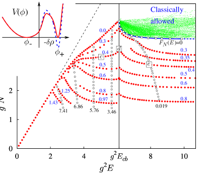
Figure 1: Solutions in $(E,N)$ plane at $\delta\rho=0.4$. Numbers near the lines with empty and filled points are the values of $T$ and $\theta$, respectively. Inset: Potential density $V(\phi)$.

We get around this obstacle by introducing the potential barrier between SA pair and perturbative states. Namely, we add negative energy density $(-\delta\rho)$ to the vacuum $\phi_{+}$, see dashed line in the inset in Fig. 1. This turns $\phi_{-}$ and $\phi_{+}$ into false and true vacua, respectively; the process of SA pair production is now interpreted as false vacuum decay false ; *false1; *false2 induced by particle collisions. The latter is a well–studied tunneling process induced_thin_wall ; *induced_thin_wall1; *induced_thin_wall2; *induced_thin_wall3; Kuznetsov . In the end of calculation we will take the limit $\delta\rho\to 0$.

The height of the potential barrier between the false and true vacua is given by the energy $E_{cb}$ of the critical bubble false — unstable static solution “sitting” on top of the barrier. The pressure $\delta\rho$ inside this bubble is balanced by the soliton–antisoliton attraction. Let us estimate the critical bubble size $d_{cb}$ at small $\delta\rho$. The attractive force $F_{att}$ between the soliton and antisoliton is proportional to the Yukawa exponent $\exp(-m_{+}d_{cb})$, where $m_{+}^{2}=V^{\prime\prime}(\phi_{+})$. Setting $F_{att}=\delta\rho$, one finds ${d_{cb}\sim-\log(\mbox{const}\cdot\delta\rho)/m_{+}}$. We see that at $\delta\rho\to 0$ the critical bubble turns into a widely separated SA pair and $E_{cb}\to 2M_{S}$, where $M_{S}$ is the soliton mass.

Figure 2: (a) Soliton–antisoliton configuration. (b) Contour in complex time. (c)—(e) Semiclassical solutions $\phi_{s}(t,x)$ at $\delta\rho=0.4$; respective values of $(E,N)$ are shown by squares with letters in Fig. 1. In particular, (c) $E<E_{cb}$, (d) $E\approx E_{cb}$, (e) $E>E_{cb}$. Color represents $\mathrm{arg}\,\phi_{s}$.

Another difficulty is met in the case of $N=2$ particles in the initial state, since states with few quanta cannot be described semiclassically. We solve this problem by Rubakov–Son–Tinyakov (RST) method RST ; *RST2, . The method is based on the assumption that as long as the number of colliding quanta is semiclassically small, $N\ll 1/g^{2}$, the leading suppression exponent $F_{N}(E)$ is universal, i.e. does not depend on $N$. In detail, consider the $N$–particle inclusive probability,

$${\cal P}_{N}(E)=\sum_{i,f}\left|\langle i;E,N|\hat{\cal S}|f;SA\rangle\right|^{2}\sim\mathrm{e}^{-F_{N}(E)/g^{2}}\;,$$ (3)

where $\hat{\cal S}$ is S–matrix. The sums in Eq. (3) run over all initial states of energy $E$ and multiplicity $N$ and final states containing SA pair and arbitrary number of quanta. RST conjecture states that the multiparticle suppression exponent $F_{N}(E)$ in Eq. (3) coincides with the two–particle exponent $F(E)$ for $N\ll 1/g^{2}$. On the other hand, at $N\gg 1$ the initial states in Eq. (3) can be described semiclassically. Thus, $F(E)$ is computed by evaluating semiclassically $F_{N}(E)$ and taking the small–$N$ limit

$$F(E)=\lim_{g^{2}N\to 0}F_{N}(E)\;.$$ (4)

It is worth noting that the conjecture (4) has been supported by field theory calculations RSTcheck ; *RSTcheck1 and proved in the context of multidimensional quantum mechanics Bonini ; LPS .

After modifying the original problem we arrived at false vacuum decay induced by collision of $N\gg 1$ particles. The latter process can be described semiclassically, as outlined below. The price to pay is the limits $\delta\rho\to 0$ and $g^{2}N\to 0$, which should be taken in the end of calculation. In particular, we are going to show that the limit $\delta\rho\to 0$ of the suppression exponent exists.

Semiclassical method for the calculation of the multiparticle probability (3) at $N\gg 1$ and $g\ll 1$ has been developed in Ref. RST . This method is based on the saddle-point evaluation  of the path integral for the probability. Below we list the boundary conditions for the complex saddle-point configuration $\phi_{s}(t,x)\in\mathbb{C}$ and give expression for $F_{N}(E)$; see Refs. [RST, , Kuznetsov, ] for derivation.

Configuration $\phi_{s}(t,x)$ satisfies classical field equation $\delta S/\delta\phi=0$ along the contour in complex time shown in Fig. 2b, where the Euclidean part corresponds to tunneling. In the asymptotic past $\phi_{s}(t,x)$ is a collection of linear waves above the false vacuum $\phi_{-}$,

$$\phi_{s}\to\phi_{-}+\int \frac{dk}{\sqrt{2\omega_{k}}}\left[a_{k}\mathrm{e}^{-i\omega_{k}t+ikx}+b_{k}^{*}\mathrm{e}^{i\omega_{k}t-ikx}\right]$$

$$\qquad\qquad\qquad\mbox{as}\;\;t\to iT-\infty\;,$$ (5)

where $\omega_{k}^{2}=k^{2}+m_{-}^{2}$, $m_{-}^{2}=V^{\prime\prime}(\phi_{-})$. The first boundary condition is relation between the amplitudes RST ,

$$a_{k}=\mathrm{e}^{-2\omega_{k}T-\theta}b_{k}\;,$$ (6a)

where $$T \theta \phi_{s}(t,x)$$ and are real parameters. In the asymptotic future contains a bubble of true vacuum. The second boundary condition is asymptotic real–valuedness:

$$\mathrm{Im}\,\phi_{s},\;\mathrm{Im}\,\partial_{t}\phi_{s}\to 0\qquad\mbox{as}\;\;t\to+\infty\;.$$ (6b)

Equations (6) are sufficient to specify complex solution $\phi_{s}(t,x)$ for given values of $T$ and $\theta$ in Eq. (6a).

Parameters $T$ and $\theta$ are related to $(E,N)$ by the saddle–point conditions [RST, , Kuznetsov, ]

$$g^{2}E={2\pi}\int dk\,\omega_{k}a_{k}b_{k}^{*}\;,\qquad g^{2}N={2\pi}\int dk\,a_{k}b_{k}^{*}\;.$$ (7)

Given the saddle–point configuration $\phi_{s}(t,x)$, one evaluates the suppression exponent,

$$F_{N}(E)=g^{2}\left(2\mathrm{Im}\,S[\phi_{s}]-2ET-N\theta\right)\;,$$ (8)

where the last two terms are due to non-trivial initial state, see Ref. Kuznetsov . Note that $\phi_{s}(t,x)$ and $F_{N}(E)$ depend on $g$, $E$, $N$ only via combinations $g^{2}N$, $g^{2}E$, see Eqs. (7).

To summarize, the recipe for calculating the suppression exponent of SA pair production in two–particle collisions is as follows. One starts at $\delta\rho>0$ by finding two–parametric family of saddle–point configurations $\phi_{s}(t,x)$ which satisfy the classical field equation and boundary conditions (6). Then one computes the values of $E$, $N$ and $F_{N}(E)$, Eqs. (7), (8), for each of these configurations. The result for the suppression exponent $F(E)$ in Eq. (1) is recovered in the limits $\delta\rho\to 0$ and $g^{2}N\to 0$.

We support the method by performing explicit calculations in the model (2) with potential shown in the inset in Fig. 1,

$$V(\phi)=\frac{1}{2}(\phi+1)^{2}\left[1-v\,W\left(\frac{\phi-1}{a}\right)\right]\;,$$ (9)

where $W(x)=\mathrm{e}^{-x^{2}}(x+x^{3}+x^{5})$, $a=0.4$ and $v$ is tuned to provide the required value of $\delta\rho$. We do not use the standard $\phi^{4}$ potential because of the chaotic properties of $\phi^{4}$ kink–antikink dynamics [kink_chaos, , solitons, ] which lead to difficulties in the semiclassical analysis chaos_semiclassical ; *chaos_semiclassical1; *chaos_semiclassical2; Onishi ; *Onishi1.

We solve the semiclassical boundary value problem numerically  using methods of Refs. Kuznetsov ; SU2 ; *SU21. Our starting point is bounce false — Euclidean solution describing spontaneous decay of false vacuum at $E=N=0$. By using the classical field equation we continue the bounce to the Minkowski parts of the contour in Fig. 2b. Then, changing $(T,\theta)$ (and thus $(E,N)$) in small steps and solving numerically the boundary value problem (6), we construct the continuous family of saddle–point configurations $\phi_{s}(t,x)$ at $E<E_{cb}$. Each configuration is represented by a point in the left part of Fig. 1. The points form the lines $\theta=\mbox{const}$ (filled points) and $T=\mbox{const}$ (empty points).

Solutions at $E<E_{cb}$, $E_{cb}\approx 2M_{S}$ have the form of distorted bounces, see Fig. 2c. Wave packets in the left part of the figure represent particles moving in the initial state; after collision, the particles back–react on the Euclidean part of solution. Using the semiclassical solutions, we calculate the multiparticle exponent $F_{N}(E)$ at $E<E_{cb}$.

We evaluate the two–particle exponent $F(E)$ by extrapolating $F_{N}(E)$  to $g^{2}N=0$ with quadratic polynomials in $g^{2}N$, cf. Eq. (4). The accuracy of extrapolation is 5%.

The probability (1) of SA pair production must vanish below the kinematic threshold $E=2M_{S}$. Let us show that, indeed, $F(E)\to+\infty$ as $\delta\rho\to 0$ in the region $E<E_{cb}\to 2M_{S}$. We recall that at small $\delta\rho$ the thin–wall approximation false is applicable and the two–particle exponent $F(E)$ can be evaluated analytically modulo $O(\delta\rho^{0})$ corrections induced_thin_wall ,

$$F=\frac{g^{4}M_{S}^{2}}{\delta\rho}\left(2\arccos{\frac{E}{2M_{S}}}-\frac{E}{M_{S}}\sqrt{1-\frac{E^{2}}{4M_{S}^{2}}}\right)\;.$$ (10)

We see that $F(E)\propto 1/\delta\rho$ at $E<2M_{S}$; this property disappears for $E\geq 2M_{S}$ where the thin–wall approximation breaks down.

Our numerical results for $\delta\rho\,\cdot F(E)$ at $g^{2}N=0$ (Fig. 3a, dashed lines) approach Eq. (10) (Fig. 3a, solid line) as $\delta\rho$ decreases and coincide with it after extrapolation to $\delta\rho=0$ (points). This gives support to our method.

The fact that $\delta\rho\,\cdot F(E)\to 0$ as $E\to 2M_{S}$, $\delta\rho\to 0$ hints that the properties of semiclassical solutions become qualitatively different at $E>E_{cb}$. This is indeed the case; in fact, our numerical procedure does not produce solutions at $E>E_{cb}$ at all. By inspecting $\phi_{s}(t,x)$ with $E\approx E_{cb}$, Fig. 2d, we see the reason for that: this solution has long, almost static part where it is close to the critical bubble. The instability of the latter makes the numerical techniques inefficient.

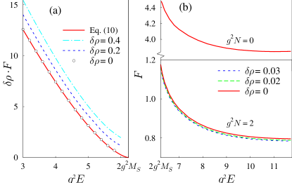
Figure 3: (a) Function $\delta\rho\cdot F(E)$ at $g^{2}N=0$, $E<2M_{S}$. (b) Suppression exponent $F_{N}(E)$ at $E>2M_{S}$.

We solve the instability problem by $\epsilon$–regularization method of Refs. [epsilon, ; *epsilon1; *epsilon2, LPS, ] which prescribes to add small imaginary term to the potential, $V(\phi)\to V_{\epsilon}(\phi,x)=V(\phi)-i\epsilon f(\phi,x)$, where $f(\phi,x)\geq 0$ at real $\phi$, ${f(\phi_{+},x)=0}$. For $\epsilon>0$ the critical bubble has complex energy and cannot be approached by $\phi_{s}(t,x)$: the energy of the latter is real due to Eq. (6b). Thus, the semiclassical solutions are no longer unstable at $\epsilon>0$ and we are able to cover the region $E>E_{cb}$ with new solutions, see Fig. 1. Using Eq. (8) and taking the limit $\epsilon\to 0$, we compute the multiparticle suppression exponent $F_{N}(E)$. The typical saddle–point configuration at $E>E_{cb}$ is shown in Fig. 2e. It still describes formation of the critical bubble ; the energy excess $E-E_{cb}$ is radiated away in the middle part of the solution.

It is worth noting that formation of classically unstable “states” is a manifestation of general tunneling mechanism proposed recently in multidimensional quantum mechanics [Onishi, , epsilon, , new_mechanism, ; *new_mechanism1, LPS, ] and quantum field theory SU2 ; Levkov ; *Levkov1.

To check the semiclassical method, we find values of $(E,N)$ corresponding to classically allowed decay of false vacuum Demidov . On the one hand, these values are obtained from the semiclassical exponent, since classical transitions correspond to $F_{N}(E)=0$. Figure 1 shows the line $F_{N}(E)=0$ obtained in this way. On the other hand, “classically allowed” values of $(E,N)$ can be obtained by studying classical solutions [Rebbi, ]. To this end, we performed Demidov Monte Carlo simulation over the sets of Cauchy data $\{\phi(0,x),\,\dot{\phi}(0,x)\}$. Starting from each set, we solved numerically the classical field equation and obtained solution $\phi_{cl}(t,x)$. We selected solutions describing transitions between the false and true vacua and computed the values of $(E,N)$, Eqs. (5), (7), for these solutions. The latter values are shown in Fig. 1 by dots which fill precisely the region bounded by our line $F_{N}(E)=0$. We conclude that the semiclassical result for $F_{N}(E)$ is reliable.

The exponent $F_{N}(E)$ is plotted in Fig. 3b at $N=2/g^{2}$ and different values of $\delta\rho$ (dashed lines). The graphs are almost indistinguishable; thus, the limit ${\delta\rho\to 0}$ exists. Extrapolating $F_{N}(E)$ to $\delta\rho=0$, we obtain the final result for the suppression exponent of SA pair production in $N$–particle collisions (solid line in Fig. 3b). The two–particle exponent $F(E)$ is recovered by extrapolating $F_{N}(E)$ to $g^{2}N=0$ (upper graph in Fig. 3b).

At high energies our suppression exponents are almost constant which is a typical behavior for collision–induced suppressions [Shifman, , SU2, , Levkov, ]. We expect that this feature holds in other models.

We end up by arguing that the method proposed in this Letter is applicable in multidimensional ($D>2$) and gauge theories. The problem with soliton–antisoliton attraction can be solved in the general case by introducing small constant force ${\bf F}$, an analog of $\delta\rho$, which drags soliton and antisoliton apart. At $|{\bf F}|\neq 0$ SA pair is separated from the perturbative sector by a potential barrier; tunneling through this barrier is a Schwinger process of spontaneous soliton–antisoliton pair creation in the external field Manton ; *Monopoles. For example, in the case of t’Hooft–Polyakov monopoles the external force is introduced by adding uniform magnetic field. Other steps of the method — RST conjecture (4) and semiclassical equations (6), (7), (8) — are explicitly general, cf. Ref. [RST, ]. In particular, suppression exponent of Schwinger process is proportional to $1/|{\bf F}|$ Manton ; *Monopoles; this enhancement vanishes schwinger_induced at $E=2M_{S}$. The final result for the semiclassical exponent of collision–induced SA pair production should be obtained by taking the limit $|{\bf F}|\to 0$ at $E>2M_{S}$.

We thank V.A Rubakov, S.M. Sibiryakov, F.L. Bezrukov and G.I. Rubtsov for discussions. This work was supported in part by grants NS-5525.2010.2; MK-7748.2010.2, grant of the “Dynasty” foundation (D.L.); RFBR-11-02-01528-a and Russian state contracts 02.740.11.0244, P520, P2598 (S.D.). Numerical calculations have been performed on the Computational cluster of the Theoretical division of INR RAS.

References

- (1) A. K. Drukier and S. Nussinov, Phys. Rev. Lett. 49, 102 (1982)
- (2) S. Dutta, D. A. Steer, and T. Vachaspati, Phys. Rev. Lett. 101, 121601 (2008)
- (3) T. Romanczukiewicz and Y. Shnir, Phys. Rev. Lett. 105, 081601 (2010)
- (4) T. Banks, G. Farrar, M. Dine, D. Karabali, and B. Sakita, Nucl. Phys. B 347, 581 (1990)
- (5) V. I. Zakharov, Phys. Rev. Lett. 67, 3650 (1991)
- (6) H. Goldberg, Phys. Lett. B 257, 346 (1991)
- (7) Upon field rescaling , the coupling constant enters the non–linear terms in the potential only, as it should.
- (8) M. B. Voloshin, I. Y. Kobzarev, and L. B. Okun, Sov. J. Nucl. Phys. 20, 644 (1975)
- (9) M. Stone, Phys. Lett. B 67, 186 (1977)
- (10) S. Coleman, Phys. Rev. D 15, 2929 (1977)
- (11) M. Voloshin and K. Selivanov, JETP Lett. 42, 422 (1985)
- (12) M. Voloshin and K. Selivanov, Sov. J. Nucl. Phys. 44, 868 (1986)
- (13) V. A. Rubakov, D. T. Son, and P. G. Tinyakov, Phys. Lett. B 278, 279 (1992)
- (14) V. G. Kiselev, Phys. Rev. D 45, 2929 (1992)
- (15) A. N. Kuznetsov and P. G. Tinyakov, Phys. Rev. D 56, 1156 (1997)
- (16) V. A. Rubakov, D. T. Son, and P. G. Tinyakov, Phys. Lett. B 287, 342 (1992)
- (17) V. A. Rubakov and M. E. Shaposhnikov, Phys. Usp. 39, 461 (1996)
- (18) For alternative approach see S. V. Iordanskii and L. P. Pitaevskii, Sov. Phys. JETP 49, 386 (1979); S. Yu. Khlebnikov, Phys. Lett. B 282, 459 (1992); D. Diakonov, V. Petrov, Phys. Rev. D 50, 266 (1994).
- (19) P. G. Tinyakov, Phys. Lett. B 284, 410 (1992)
- (20) A. H. Mueller, Nucl. Phys. B 401, 93 (1993)
- (21) G. F. Bonini, A. G. Cohen, C. Rebbi, and V. A. Rubakov, Phys. Rev. D 60, 076004 (1999)
- (22) D. G. Levkov, A. G. Panin, and S. M. Sibiryakov, J. Phys. A: Math. Theor. 42, 205102 (2009)
- (23) The saddle–point method is justified at small when the integrand in the path integral rapidly oscillates, cf. Eq. (2).
- (24) D. K. Campbell, J. F. Schonfeld, and C. A. Wingate, Physica D 9, 1 (1983)
- (25) O. Bohigas, S. Tomsovic, and D. Ullmo, Phys. Rep. 223, 43 (1993)
- (26) A. Shudo and K. S. Ikeda, Phys. Rev. Lett. 74, 682 (1995)
- (27) A. Shudo and K. S. Ikeda, Phys. Rev. Lett. 76, 4151 (1996)
- (28) T. Onishi, A. Shudo, K. S. Ikeda, and K. Takahashi, Phys. Rev. E 64, 025201 (2001)
- (29) T. Onishi, A. Shudo, K. S. Ikeda, and K. Takahashi, Phys. Rev. E 68, 056211 (2003)
- (30) We discretize Eqs. (6), (7), (8) by introducing uniform lattice of extent . Precision of discretization is kept smaller than ; it is controlled by changing the lattice size and keeping track of energy conservation. Linear evolution in Eq. (5) holds with accuracy smaller than . Extrapolation produces relative errors in of order .
- (31) F. Bezrukov, D. Levkov, C. Rebbi, V. Rubakov, and P. Tinyakov, Phys. Rev. D 68, 036005 (2003)
- (32) F. Bezrukov, D. Levkov, C. Rebbi, V. Rubakov, and P. Tinyakov, Phys. Lett. B 574, 75 (2003)
- (33) One can argue RST ; Levkov that as , so we use only the first two terms in Eq. (8).
- (34) F. Bezrukov and D. Levkov, arXiv:quant-ph/0301022 (2003)
- (35) F. Bezrukov and D. Levkov, JETP 98, 820 (2004)
- (36) D. G. Levkov, A. G. Panin, and S. M. Sibiryakov, Phys. Rev. Lett. 99, 170407 (2007)
- (37) The critical bubble decays in the right part of Fig. 2e due to regularization .
- (38) K. Takahashi and K. S. Ikeda, J. Phys. A: Math. Gen. 36, 7953 (2003)
- (39) K. Takahashi and K. S. Ikeda, EPL 71, 193 (2005)
- (40) D. G. Levkov and S. M. Sibiryakov, Phys. Rev. D 71, 025001 (2005)
- (41) D. G. Levkov and S. M. Sibiryakov, JETP Lett. 81, 53 (2005)
- (42) S. V. Demidov and D. G. Levkov, JHEP 1106, 016 (2011)
- (43) C. Rebbi and R. Singleton, Phys. Rev. D 54, 1020 (1996)
- (44) M. Maggiore and M. Shifman, Nucl. Phys. B 371, 177 (1992)
- (45) N. S. Manton, Nucl. Phys. B 126, 525 (1977)
- (46) I. K. Affleck and N. S. Manton, Nucl. Phys. B 194, 38 (1982)
- (47) A. K. Monin, JHEP 0510, 109 (2005)