A large scale coherent magnetic field:
interactions with free streaming particles and limits from the CMB

Abstract:

We study a homogeneous and nearly-isotropic Universe permeated by a homogeneous magnetic field. Together with an isotropic fluid, the homogeneous magnetic field, which is the primary source of anisotropy, leads to a plane-symmetric Bianchi I model of the Universe. However, when free-streaming relativistic particles are present, they generate an anisotropic pressure which counteracts the one from the magnetic field such that the Universe becomes isotropized. We show that due to this effect, the CMB temperature anisotropy from a homogeneous magnetic field is significantly suppressed if the the neutrino masses are smaller than 0.3 eV.

1 Introduction

On very large scales, the observed Universe is well approximated by a homogeneous and isotropic Friedmann solution of Einstein’s equations. This is best verified by the isotropy of the Cosmic Microwave Background (CMB). The small fluctuations observed in the CMB temperature are fully accounted for by the standard model of structure formation from small initial fluctuations which are generated during an inflationary phase. Nevertheless, these small fluctuations are often used to limit other processes or components which may be present in the early Universe, like e.g. a primordial magnetic field.

The generation of the magnetic fields observed in galaxies and clusters [1] is still unclear. It has been shown that phase transitions in the early Universe, even if they do generate magnetic fields, have not enough power on large scale to explain the observed large scale coherent fields [2]. These findings suggest that primordial magnetic fields must be correlated over very large scales.

In this paper, we discuss limits on fields which are coherent over a Hubble scale and which we can therefore treat as a homogeneous magnetic field permeating the entire Universe. We want to derive limits on a homogeneous field from CMB anisotropies. This question has been addressed in the past [3] and limits on the order of $B\,\raisebox{-2.58334pt}{$\buildrel<\over{\sim}$}\,2\times 10^{-9}$ Gauss have been derived from the CMB anisotropies [4]. A similar limit can also be obtained from Faraday rotation [5, 6].

We show that the limits from the CMB temperature anisotropy actually are invalid if free streaming neutrinos with masses $m_{\nu}<T_{\rm dec}$ are present, where $T_{\rm dec}$ denotes the photon temperature at decoupling. This is the case if the neutrino masses are not degenerate, i.e. the largest measured mass splitting is of the order of the largest mass, hence $m_{\nu}\,\raisebox{-2.58334pt}{$\buildrel<\over{\sim}$}\,0.04$eV. The same effect can be obtained from any other massless free streaming particle species, like e.g. gravitons, if they contribute sufficiently to the background energy density. This is due to the following mechanism which we derive in detal in this paper: In an anisotropic Bianchi-I model, free streaming relativistic particles develop an anisotropic stress. If the geometric anisotropy is due to a magnetic field, which scales exactly like the anisotropic stress of the massless particles, this anisotropic stress cancels the one from the magnetic field and the Universe is isotropized. Hence the quadrupole anisotropy of the CMB due to the magnetic field is erased. This ‘compensation’ of the magnetic field anisotropic stress by free-streaming neutrinos has also been seen in the study of the effects of stochastic magnetic fields on the CMB [7, 8, 9, 10] for the large scale modes. In our simple analysis the mechanism behind it finally becomes clear.

The limits from Faraday rotation are not affected by our arguments.

In the next section we derive the CMB anisotropies in a Bianchi I Universe. In Section 3 we show that relativistic free streaming neutrinos in a Bianchi I model develop anisotropic stresses and that these back-react to remove the anisotropy of the Universe if the latter is due to a massless mode. In Section 4 we discuss isotropization due to other massless free streaming particles, with special attention to a gravitational wave background. In Section 5 we conclude.

2 Effects on the CMB from a constant magnetic field in an ideal fluid Universe

We consider a homogeneous magnetic field in $z-$direction, ${\mathbf{B}}=B\bm{e}_{z}$ in a Universe filled otherwise with an isotropic fluid consisting, e.g. of matter and radiation. The metric of such a Universe is of Bianchi type I,

$$ds^{2} = -dt^{2}+a_{\perp}^{2}(t)(dx^{2}+dy^{2})+a_{\parallel}^{2}(t)\,dz^{2}\,,$$ (1)

where $t$ is cosmic time. The Einstein equations in cosmic time read

$$2\frac{\dot{a}_{\parallel}}{a_{\parallel}}\frac{\dot{a}_{\perp}}{a_{\perp}}+\left(\frac{\dot{a}_{\perp}}{a_{\perp}}\right)^{2} = 8\pi G\rho~{},$$ (2)

$$\frac{\ddot{a}_{\parallel}}{a_{\parallel}}+\frac{\ddot{a}_{\perp}}{a_{\perp}}+\frac{\dot{a}_{\parallel}}{a_{\parallel}}\frac{\dot{a}_{\perp}}{a_{\perp}} = -8\pi GP_{\perp}~{},$$ (3)

$$2\frac{\ddot{a}_{\perp}}{a_{\perp}}+\left(\frac{\dot{a}_{\perp}}{a_{\perp}}\right)^{2} = -8\pi GP_{\parallel}~{}.$$ (4)

The dot denotes the derivative with respect to $t$. We have introduced the total energy density $\rho=\rho_{B}+\rho_{m}+\rho_{\gamma}+\rho_{\nu}+\rho_{\Lambda}$, where $\rho_{B}=B^{2}/8\pi$ is the energy density in the magnetic field, and $\rho_{m},\rho_{\gamma},\rho_{\nu},\rho_{\Lambda}$ are as usual the energy densities of matter (assumed to be baryons and cold dark matter), photons, neutrinos, and dark energy (assumed to be a cosmological constant), respectively.

All the above constituents of the Universe, except matter (which is assumed to be pressureless) also contribute to the pressure components $P_{\parallel},P_{\perp}$. The contribution from the magnetic field is intrinsically anisotropic and given by

$$P_{B,\perp}=-P_{B,\parallel}=\rho_{B}\,,$$ (5)

as can be read off from the corresponding stress-energy tensor. Note that the magnetic field $B$ decays as $a_{\perp}^{-2}$, so that $\rho_{B}$ scales as $a_{\perp}^{-4}$.

For later reference we define an ‘average’ scale factor

$$a\equiv a_{\perp}^{2/3}a_{\parallel}^{1/3}\,,$$ (6)

which is chosen such that it correctly describes the volume expansion.

Let us also introduce the expansion rates $H_{\perp}=\dot{a}_{\perp}/a_{\perp}$ and $H_{\parallel}=\dot{a}_{\parallel}/a_{\parallel}$. The anisotropic stress of the homogeneous magnetic field sources anisotropic expansion, which can be expressed as the difference of the expansion rates, $\Delta H=H_{\perp}-H_{\parallel}$. We combine eqs. (4) and (3) to obtain an evolution equation for $\Delta H$,

$$\dot{\Delta H}+\left(2H_{\perp}+H_{\parallel}\right)\Delta H=8\pi G\left(P_{\perp}-P_{\parallel}\right)\,.$$ (7)

This pressure difference is actually simply the anisotropic stress. More precisely,

$${\Pi_{i}}^{j} \equiv {T_{i}}^{j}-P{\delta_{i}}^{j}\,,\qquad P=T_{i}^{i}/3=(2P_{\perp}+P_{\parallel})/3\,,$$

$${\Pi_{1}}^{1} = {\Pi_{2}}^{2}=P_{\perp}-P=\frac{1}{3}\left(P_{\perp}-P_{\parallel}\right)\,,\quad{\Pi_{3}}^{3}=P_{\parallel}-P=-\frac{2}{3}\left(P_{\perp}-P_{\parallel}\right)\,.$$ (8)

At very high temperatures, both photons and neutrinos are tightly coupled to baryons. Their pressure is isotropic and thus their contribution to the right-hand-side of (7) vanishes. The collision term in Boltzmann’s equation tends to isotropize their momentum-space distribution. Under these conditions the only source of anisotropic stress is the magnetic field. The above equation can then easily be solved to leading order in $\Delta H$, as will be carried out in section 3.

However, as soon as the neutrinos decouple and start to free-stream, their momentum-space distribution will be affected by the anisotropic expansion caused by the magnetic field and thus they will develop anisotropic stress. As we will show, the neutrino anisotropic stress counteracts the one from the magnetic field. This behavior will be maintained until the neutrinos become non-relativistic, then their pressure decays. For the temperature anisotropy in the CMB it is relevant whether this happens before or after photon decoupling. This depends, of course, on the neutrino masses.

We introduce the energy density parameters

$$\Omega_{x}(t)\equiv\frac{8\pi G\rho_{x}(t)}{3H^{2}(t)}=\frac{\rho_{x}(t)}{\rho_{c}(t)}\;,$$

corresponding respectively to the magnetic field, matter and radiation etc., such that e.g. $\Omega_{B}=B^{2}/8\pi\rho_{c}$, $\Omega_{m}=\rho_{m}/\rho_{c}$ and $\Omega_{\gamma}=\rho_{\gamma}/\rho_{c}$. Here we define the ‘average’ Hubble parameter by

$$H^{2}\equiv\frac{1}{3}\left[\left(\frac{\dot{a}_{\perp}}{a_{\perp}}\right)^{2}+2\frac{\dot{a}_{\perp}\dot{a}_{\parallel}}{a_{\perp}a_{\parallel}}\right]\;.$$ (9)

With this, eq. (2), implies

$$\Omega_{\rm T}\equiv\Omega_{B}+\Omega_{\gamma}+\Omega_{\nu}+\Omega_{m}+\Omega_{\Lambda}=1\quad\mbox{ at all times.}$$ (10)

As an alternative, one could have defined the ‘average’ Hubble parameter as

$$H_{a}\equiv\frac{1}{3}\left[2\frac{\dot{a}_{\perp}}{a_{\perp}}+\frac{\dot{a}_{\parallel}}{a_{\parallel}}\right]\;.$$

It can easily be verified that the difference between these definitions is of the order of the small quantity $\Delta H=H_{\perp}-H_{\parallel}$. More precisely,

$$H^{2} = H_{a}^{2}\left[1-\frac{2}{3}\frac{\Delta H}{H_{a}}-\frac{1}{3}\left(\frac{\Delta H}{H_{a}}\right)^{2}\right]\,.$$ (11)

We shall mainly use the definition which yields the constraint (10).

The scaling of the energy densities corresponding to every species follows from the stress energy conservation of every single fluid

$$\rho_{\gamma}=\rho_{\gamma}^{0}\left(\frac{a_{0}}{a}\right)^{4}\,,\quad\rho_{m}=\rho_{m}^{0}\left(\frac{a_{0}}{a}\right)^{3}\,,\quad\rho_{B}=\rho_{B}^{0}\left[\frac{a_{\perp}(t_{0})}{a_{\perp}}\right]^{4}\,.$$ (12)

To obtain the above behavior for radiation, it is important to impose that the fluid is ideal, i.e. that pressure is isotropic. This is the case if there are sufficiently many collisions, but does not hold for free streaming particles as we shall see in the next section.

At a fixed initial time one may set $a_{\perp}=a_{\parallel}$ as initial condition. Motivated by observations, we assume that the scale factor difference always remains small,

$$\frac{a_{\perp}-a_{\parallel}}{a}\equiv\delta\ll 1\;.$$ (13)

To first order in $\Delta H\ll H$, as long as the magnetic field is the only anisotropic component, eq. (7) becomes (see also [11])

$$\dot{\Delta H}+3H\Delta H=8\pi G\left(P_{\perp}-P_{\parallel}\right)=6H^{2}\Omega_{B}\,.$$ (14)

In the following we consider both $\Omega_{B}$ and $\Delta H$ as small quantities and want to calculate effects to first order in them. To first order, $\rho_{B}\propto a^{-4}\propto\rho_{\gamma}$. We can therefore introduce the ratio

$$r=\frac{\rho_{B}}{\rho_{\gamma}}=\frac{\Omega_{B}}{\Omega_{\gamma}}\,,$$ (15)

which (to first order) is constant.

In fig. 1 we plot the scale factor difference $\delta_{0}-\delta$ and $\Delta H/H$ as functions of the temperature in a first stage where neutrinos, photons and baryons are all tightly coupled and the magnetic field is the only source of anisotropy.

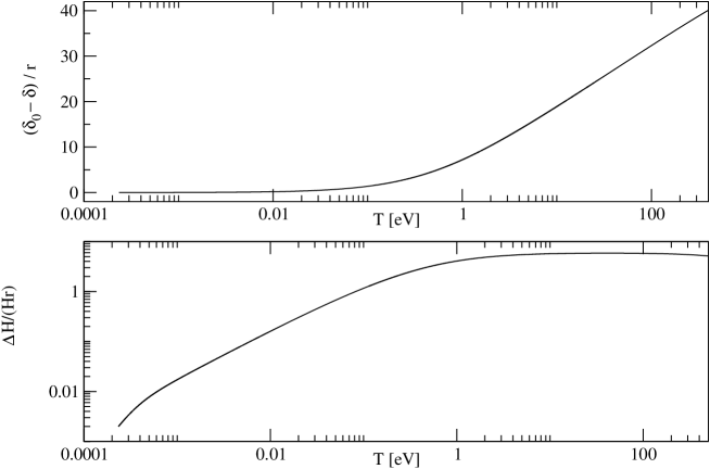
Figure 1: Temperature evolution of the scale factor difference $\delta_{0}-\delta$ and $\Delta H/H$ in units of $r=\Omega_{B}/\Omega_{\gamma}$ when no free-streaming particle compensates the anisotropy produced by the magnetic field anisotropic stress. Here $\delta_{0}$ denotes the scale factor difference $\delta$ today. The evolution of the ‘average’ scale factor $a$ is the one of a $\Lambda$CDM Universe. As it is shown in section 3, $\Delta H/H$ is constant during the radiation dominated era and $\delta$ is growing. During the matter dominated era $\Delta H/H$ is decaying, $\Delta H/H\propto 1/a\propto T$, and $\delta$ asymptotes to a constant.

2.1 Lightlike geodesics in Bianchi I

Let us now determine the CMB anisotropies in a Bianchi I Universe. We are not interested in the usual anisotropies from primordial perturbations, which we disregard in our treatment, but we concentrate on the effect of the global anisotropy, which to leading order will result in a temperature quadrupole.

We choose the tetrad basis $e_{0}=\partial_{t}$, $e_{i}=a_{\perp}^{-1}\partial_{i}$ for $i=1,2$ and $e_{3}=a_{\parallel}^{-1}\partial_{3}$. The dual basis of 1-forms is given by $\theta^{0}=dt$, $\theta^{i}=a_{\perp}dx^{i}$, for $i=1,2$ and $\theta^{3}=a_{\parallel}dx^{3}$. The first structure equation,

$$d\theta^{a}+{\omega^{a}}_{b}\wedge\theta^{b}=0\,,$$

yields

$${\omega^{i}}_{0} = \frac{\dot{a}_{\perp}}{a_{\perp}}\theta^{0}\;,\quad i=1,2\,,\qquad{\rm and}\quad{\omega^{3}}_{0}=\frac{\dot{a}_{\parallel}}{a_{\parallel}}\theta^{0}\,.$$ (16)

The other non-vanishing connection 1-forms are determined by anti-symmetry, $\omega_{ab}=-\omega_{ba}$. After photon decoupling, the photon 4-momentum ${\bm{p}}=p^{a}\bm{e}_{a}$ satisfies the geodesic equation

$$\frac{dp^{a}}{d\lambda}+\omega_{\phantom{1}c}^{a}(\bm{e}_{b})\,p^{b}\,p^{c}=0\,.$$ (17)

Considering the constraint relation for massless particles $p_{a}p^{a}=0$ and setting $\alpha T_{0}\equiv p^{0}=p=\sqrt{\sum_{i=1}^{3}(p^{i})^{2}}$, where $T_{0}$ is a constant with the dimension of energy (or temperature) that multiplies all the components $p^{a}$, the above equation is solved by

$$\left(p^{a}\right)=T_{0}\left(\alpha,\frac{n^{1}}{a_{\perp}},\frac{n^{2}}{a_{\perp}},\frac{n^{3}}{a_{\parallel}}\right)\,,$$ (18)

where $n$ is a unit vector in the direction of the particle momentum and $\alpha$ is determined by the condition $p_{a}p^{a}=0$.

$$n^{1}=\sin\theta\sin\phi\;,\quad n^{2}=\sin\theta\cos\phi\quad\mbox{ and }\quad n^{3}=\cos\theta\;.$$

The temperature of photons in such an anisotropic Universe for a comoving observer, $u=\partial_{t}$, is then given by

$$T(t,\theta)=\eta_{ab}u^{a}p^{b}=p^{0}=T_{0}\alpha=T_{0}\sqrt{\frac{\sin^{2}\theta}{a_{\perp}^{2}}+\frac{\cos^{2}\theta}{a_{\parallel}^{2}}}\simeq\frac{T_{0}}{a}\left[1+\delta\cos^{2}\theta+{\cal O}(\delta^{2})\right]\,.$$ (19)

We set

$$\bar{T}=\frac{1}{4\pi}\int T(t,\theta)\sin\theta d\theta d\phi=\frac{T_{0}}{a}\left[1+\frac{1}{3}\delta+{\cal O}(\delta^{2})\right]$$

to be the temperature averaged over directions. Note that for $\delta=0$ and $a_{0}=1$, $T_{0}$ is simply the CMB temperature at time $t_{0}$. For the temperature fluctuations to first order in $\delta$ we obtain

$$\frac{\Delta T}{T}\equiv\frac{T(t,\theta)-\bar{T}}{\bar{T}}=\frac{1}{3}\delta(3\cos^{2}\theta-1)+{\cal O}(\delta^{2})=\delta\frac{2}{3}\sqrt{\frac{4\pi}{5}}Y_{20}({\mathbf{n}})+{\cal O}(\delta^{2})\;.$$ (20)

Hence, to lowest order in $\delta$ a homogeneous magnetic field generates a quadrupole which is given by

$$C_{2}=\frac{1}{5}\sum_{m=-2}^{2}|a_{2m}|^{2}=\frac{1}{5}|a_{20}|^{2}=\frac{16\pi}{225}\delta^{2}\simeq 0.22\times\delta^{2}\;.$$ (21)

Of course, in principle one can set $\delta(t_{1})=0$ at any given moment $t_{1}$ which then leads to $\frac{\Delta T}{T}(t_{1})=0$. However, for the CMB we know that photons start free-streaming only at $t_{\rm dec}$ when they decouple from electrons. Before that, scattering isotropizes the photon distribution and no quadrupole can develop. In other words, we have to make sure that the anisotropy-induced quadrupole is fixed to zero at decoupling and only appears as a result of differential expansion between last scattering and today. This can be taken into account by simply choosing the initial condition $\delta(t_{\rm dec})=0$. Without this initial condition we have to replace $\delta(t)$ by $\delta(t)-\delta(t_{\rm dec})$ in eq. (21) . The general result for the CMB quadrupole today is therefore

$$C_{2}=\frac{16\pi}{225}\left[\delta(t_{0})-\delta(t_{\rm dec})\right]^{2}\;.$$ (22)

2.2 The Liouville equation

At this stage it is straightforward to check that the exact expression found above for the temperature, eq. (19), satisfies the Liouville equation for photons (see, e.g.  [12])

$$p^{a}\bm{e}_{a}(f_{\gamma})-\omega^{i}_{\phantom{1}b}({\bm{p}})p^{b}\frac{\partial f_{\gamma}}{\partial p^{i}}=0\,,$$ (23)

when we make the following Ansatz for the distribution function of massless bosonic particles in our Bianchi I Universe

$$p_{\bot}\equiv\sqrt{(p^{1})^{2}+(p^{2})^{2}}\,,\quad p_{\parallel}=p^{3},\quad p=\sqrt{p_{\bot}^{2}+p_{\parallel}^{2}}=p^{0}\,,$$ (24)

$$f_{\gamma}(t,T)=\frac{N_{\gamma}}{(2\pi)^{3}}\frac{1}{{\rm e}^{p/T}-1},\qquad T=T(t,\theta)\,.$$ (25)

Indeed, using eqs. (16), we find the following differential equation for the temperature $T$

$$\frac{\partial f_{\gamma}}{\partial T}\frac{\partial T}{\partial t}-\frac{\dot{a}_{\perp}}{a_{\perp}}\frac{\partial f_{\gamma}}{p_{\bot}}p_{\bot}-\frac{\dot{a}_{\parallel}}{a_{\parallel}}\frac{\partial f_{\gamma}}{\partial p_{\parallel}}p_{\parallel}=0\,.$$ (26)

With (25) this can be written as

$$\frac{\dot{T}}{T}+\frac{\dot{a}_{\perp}}{a_{\perp}}\left(\frac{p_{\bot}}{p}\right)^{2}+\frac{\dot{a}_{\parallel}}{a_{\parallel}}\left(\frac{p_{\parallel}}{p}\right)^{2}=0\,.$$ (27)

The time behavior of the different components of the photon momentum are given by eq. (18) and one immediately sees that expression (19) for the temperature solves the above differential equation.

Moreover, defining the time dependent unit vectors $\hat{p}^{i}\equiv p^{i}/p$ and the shear tensor

$$\sigma_{ab}\equiv\vartheta_{ab}-\frac{1}{3}\vartheta_{c}^{c}h_{ab}\ ,~{}~{}\mbox{ where }\vartheta_{ab}\equiv\frac{1}{2}\left(\nabla_{a}u_{b}+\nabla_{b}u_{a}\right)~{}\mbox{ and }~{}h_{ab}\equiv\eta_{ab}+u_{a}u_{b}\,,$$

one can rewrite the above Liouville equation as

$$(\tilde{p})^{\dot{}}=-\tilde{p}\sigma_{ij}\hat{p}^{i}\hat{p}^{j}\,,$$ (28)

where $\tilde{p}$ denotes the redshift-corrected photon energy defined as $\tilde{p}\equiv ap$. This last expression agrees with the corresponding equation given in [13].

Using the expression for the distribution function of massless fermions, we can also compute the pressure of neutrinos once they start free-streaming. Indeed, given the fact that neutrinos can be considered massless before they become non-relativistic, their geodesic equation has the same solution as the one for photons found above, therefore we immediately obtain the time behavior of their temperature in an anisotropic Bianchi I background. Taking also into account the fact that neutrinos are fermions, their distribution function reads

$$f_{\nu}(t,T)=\frac{N_{\nu}}{(2\pi)^{3}}\frac{1}{{\rm e}^{p/T}+1},\quad\mbox{with}\quad T(t,\theta)=\frac{T_{\nu}}{a}\left[1+\delta\cos^{2}\theta+{\cal O}(\delta^{2})\right]\,.$$ (29)

Note that the parameter $T$ appearing in the neutrino distribution function in not a temperature in the thermodynamical sense as the neutrinos are not in thermal equilibrium. It is simply a parameter in the distribution function and its time evolution has been determined by requiring the neutrinos to move along geodesics i.e. to free-stream.

This distribution function remains valid also in the case where neutrinos are massive, i.e. $T_{\nu}<m_{\nu}$. The only difference is that the relation $p^{0}=p$ changes to $p^{0}=\sqrt{p^{2}+(m_{\nu}a)^{2}}$ which of course affects the momentum integrals for the neutrino energy density and pressure.

The energy $T_{\nu}/a_{0}$ is the present neutrino ‘temperature’ in the absence of a homogeneous magnetic field ($\delta=0$). The energy density $\rho_{\nu}$ and the pressure $P_{\nu,i}$ in direction $i$ with respect to our orthonormal basis are

$$\rho_{\nu} = N_{\nu}\int d^{3}p\,f_{\nu}(t,T)p^{0}$$ (30)

$$P_{\nu,i} = N_{\nu}\int d^{3}p\,f_{\nu}(t,T)\,\frac{p_{i}^{2}}{p^{0}}\,.$$ (31)

Calculating the integral (31) for relativistic neutrinos to first order in $\delta$ in the directions perpendicular and parallel to the magnetic field direction, one finds for the neutrino anisotropic stress in the ultra-relativistic limit

$$P_{\nu,\perp}-P_{\nu,\parallel}\simeq-\frac{8}{15}\rho_{\nu}\left(\delta-\delta_{\ast}\right)\,,$$ (32)

where $\delta_{\ast}$ is the value of $\delta$ at neutrino decoupling and can be fixed to zero for convenience.

The temperature dependence of the neutrino pressure is shown in fig. 2. To leading order, this also gives the temperature dependence of the neutrino anisotropic stress. From the plot it is clear how the pressure scales as $a^{-4}$ as long as the neutrinos are ultra-relativistic. Once they have become effectively non-relativistic, their pressure decays more rapidly, as $a^{-5}$. The break in the power law is not precisely at $T=m_{\nu}$, but at a somewhat lower temperature. Because the neutrinos still have the highly relativistic Fermi-Dirac distribution from the time of their thermal freeze-out, it takes some additional redshift until they behave effectively non-relativisic. This will have some effect on the estimates for the residual CMB quadrupole, as we shall see in sec. 3, in particular the discussion of fig. 5.

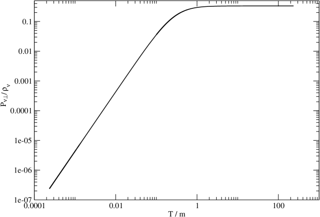
Figure 2: Temperature evolution of the neutrino pressure $P_{\nu,\perp}$ normalized to the neutrino energy density $\rho_{\nu}$. The temperature is given in units of the neutrino mass. Note that the break in the power law is not at $T=m$, but at somewhat lower temperature. This is due to the highly relativistic Fermi-Dirac distribution of the neutrinos, see also the discussion of fig. 5 in sec. 3.3.

3 Neutrino free-streaming and isotropization

3.1 Massless free-streaming neutrinos

We now calculate the effect of free-streaming neutrinos perturbatively, i.e. to first order in $\delta$, $\Delta H/H$ and $\Omega_{B}$. We linearize eq. (7), taking into account the contribution of a free-streaming relativistic component to the right-hand side. We have shown that this contribution, to leading order in $\delta$, is given by eq. (32). Furthermore, up to $\mathcal{O}(\delta^{2})$ corrections, $\delta$ is just the integral of $\Delta H$,

$$\int_{t_{\ast}}^{t}\!\Delta H(t^{\prime})dt^{\prime}=\ln\frac{a_{\perp}\left(t\right)}{a_{\parallel}\left(t\right)}-\ln\frac{a_{\perp}\left(t_{\ast}\right)}{a_{\parallel}\left(t_{\ast}\right)}\simeq\delta-\delta_{\ast}~{},$$ (33)

so that to first order we can identify $\Delta H\simeq\dot{\delta}$.

Inserting this back into eq. (7) we find, to linear order in $\delta$,

$$\ddot{\delta}+3H\dot{\delta}+\frac{8}{5}H^{2}\Omega_{\nu}\left(\delta-\delta_{\ast}\right)=6H^{2}\Omega_{B}~{}.$$ (34)

Note that, because we are working at linear order, it is not important with respect to which scale factor $H,\Omega_{\nu}$ and $\Omega_{B}$ are defined in (34). We will now give analytic solutions to this equation for different regimes in the evolution of the Universe.

Let us begin at very high temperature where the neutrinos are still strongly coupled to baryons. In this case they do not contribute to eq. (34) since their pressure is isotropic $(P_{\nu,\perp}-P_{\nu,\parallel}\sim 0)$ given the high rate of collisions. Furthermore, since we are in the radiation dominated era $(a\propto t^{1/2})$, we have $H=1/2t$, and $\Omega_{B}$ is constant. The solution to eq. (34) in this case is

$$\dot{\delta}(t)=\Delta H(t)=\frac{3\Omega_{B}}{t}+\frac{C}{t^{3/2}}~{}.$$ (35)

The dimensionless quantity $\Delta H/H$ hence asymptotes to a constant, since the homogeneous piece decays like $a^{-1}$:

$$\frac{\Delta H}{H}\rightarrow 6\Omega_{B}~{}.$$ (36)

$\Delta H$ soon becomes insensitive to the initial conditions and only depends on $\Omega_{B}$. This also shows that in the absence of an anisotropic source ($\Omega_{B}=0$), the expanding Universe isotropizes. Integrating this equation and remembering that $\Omega_{B}=$ constant to first order in a radiation dominated Universe, we obtain

$$\delta(t)-\delta(t^{\prime})=3\Omega_{B}\ln(t/t^{\prime})\,.$$ (37)

As the Universe reaches a temperature of roughly $1.4$ MeV, the neutrinos decouple and begin to free-stream, giving rise to the corresponding term in eq. (34). In the radiation dominated era, $\Omega_{\nu}$ remains constant as long as neutrinos are ultra-relativistic. This is certainly true for temperatures well above a few eV. In this regime, the general solution of eq. (34) is given by

$$\delta(t)-\delta_{\ast}=\frac{15}{4}\frac{\Omega_{B}}{\Omega_{\nu}}+t^{-1/4}\left(C_{+}t^{i\sqrt{2\Omega_{\nu}/5-1/16}}+C_{-}t^{-i\sqrt{2\Omega_{\nu}/5-1/16}}\right)~{}.$$ (38)

For $\Omega_{\nu}>5/32$, the homogeneous part is oscillating with a damping envelope $\propto t^{-1/4}\propto a^{-1/2}$. This means that $\Delta H=\dot{\delta}$ will decay within a few Hubble times, which is a matter of seconds at the temperatures we are talking about. After that, $\delta-\delta_{\ast}$ will remain constant at the value of $\left(15/4\right)\Omega_{B}/\Omega_{\nu}$ until the neutrinos become non-relativistic. Then their pressure drops dramatically and so does their anisotropic stress. Until this time, the Universe expands isotropically, because the anisotropic stress of the magnetic field is precisely cancelled by the one of the neutrinos. Remember that a constant $\delta$ can always be absorbed in a re-scaling of the coordinates and has no physical effect. Fig. 3 shows the temperature evolution of $\delta-\delta_{\ast}$ in the radiation dominated era from neutrino decoupling until $T=100\mathrm{eV}$.

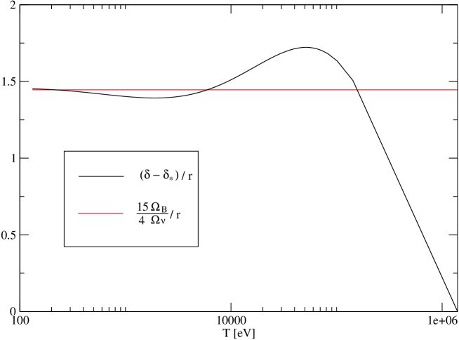
Figure 3: Temperature evolution of $\delta-\delta_{\ast}$ from neutrino decoupling to $T=100\mathrm{eV}$. After decoupling, $\delta-\delta_{\ast}$ begins to oscillate with a decreasing amplitude around the constant $\frac{15}{4}\frac{\Omega_{B}}{\Omega_{\nu}}$, as predicted by the analytic solution (38). This qualitative behavior is independent of the initial conditions.

This mechanism rests on two important facts. Firstly, as long as neutrinos are ultra-relativistic, they redshift in the same way as the magnetic field, meaning that $\Omega_{B}/\Omega_{\nu}$ is constant. Once the anisotropic stress of the neutrinos has adjusted to the magnetic field, their sum remains zero independent of the expansion of the Universe which is now in a Friedmann phase. Secondly, the efficiency of the effect hinges on the absolute value of $\Omega_{\nu}$. In the radiation dominated era (after positron annihilation), we have $\Omega_{\nu}\simeq 0.4$ so that $\Omega_{\nu}>5/32$, and hence the system behaves as an underdamped oscillator with a damping envelope $\propto t^{-1/4}$. Had the density parameter of the free-streaming particles been less than $5/32$, the behavior would be that of an overdamped oscillator. As it is evident from eq. (38), for $\Omega_{\nu}\ll 5/32$ there would be a mode which decays extremely slowly, roughly as $t^{-4\Omega_{\nu}/5}$. This is why a strongly subdominant free-streaming component cannot damp the anisotropy efficiently. As we shall discuss in section 4, a primordial gravitational wave background could play the role of such a free-streaming component if $\Omega_{GW}\gtrsim 5/32$.

3.2 Massive neutrinos

The neutrinos become non-relativistic roughly at the time when their temperature drops below their mass scale. Current bounds on the neutrino mass [14] are such that the highest-mass eigenstate is somewhere between $\sim 1$ eV and $\sim 0.04$ eV. Since the neutrino mass splitting is much below $1$ eV, an eigenstate close to the upper bound would mean that the neutrinos are almost degenerate and hence become non-relativistic all at the same time. If this happens before photon decoupling, i.e., if $m_{\nu}>0.3$ eV, the isotropization effect will not be present and the CMB will be affected by the anisotropic expansion sourced by the magnetic field. However, if the neutrinos remain ultra-relativistic until long after photon decoupling, the CMB quadrupole due to anisotropic expansion will be reduced because the neutrinos maintain expansion isotropic until they become non-relativistic.

In order to quantify this statement, we repeat the above calculations for the matter dominated era. For our purposes, this is a reasonable approximation for the time between photon decoupling and today. At decoupling, radiation is already subdominant, and on the other hand vacuum energy only begins to dominate at redshift $z\sim 0.5$. We therefore expect that both give small corrections only.

For completeness, we also give the solution of eq. (34) in a matter dominated Universe for the case where we ignore any contributions from free-streaming particles (neutrinos and, after decoupling, also photons). During matter domination we have $H=2/3t$ and $\Omega_{B}\propto a^{-1}\propto t^{-2/3}$. The solution to (14) hence reads

$$\dot{\delta}(t)=\Delta H(t)=\frac{8\Omega_{B}(t)}{t}+\frac{C}{t^{2}}~{}.$$ (39)

The homogeneous mode again decays more rapidly than the particular solution, so that the dimensionless quantity $\Delta H/H$ is again asymptotically proportional to $\Omega_{B}$. Instead of eqs. (36), (37), we have

$$\frac{\Delta H}{H}\rightarrow 12\Omega_{B}~{},\qquad\delta(t)-\delta(t_{\rm eq})=\int_{t_{\rm eq}}^{t}\Delta Hdt\simeq 12\left[\Omega_{B}(t_{\rm eq})-\Omega_{B}(t)\right]\;.$$ (40)

Let us now take into account a free-streaming component. We want to estimate the effect on the photon distribution function caused by anisotropic expansion in two cases. Case A: the neutrinos become non-relativistic before photon decoupling. Case B: the neutrinos become non-relativistic after photon decoupling. As an approximation, we assume that this happens instantaneously to all neutrino species, such that the contribution of neutrinos to eq. (34) disappears abruptly. We know that the neutrinos are in fact spread out in momentum space and also have a certain spread in the mass spectrum, so in reality this will be a gentle transition. However, we only want to estimate the order of magnitude of the effect and are not interested in these details at this point. More precice numerical results will be presented in sec. 3.3. Let us consider case A first.

3.2.1 Case A: neutrinos become non-relativistic before photon decoupling

We know that $\Delta H$ is very nearly zero when the neutrinos become non-relativistic. After that, $\Delta H/H$ will start to grow again to approach the value $6\Omega_{B}$ during radiation domination and $12\Omega_{B}$ during matter domination. As boundary condition at photon decoupling, we will hence assume $\Delta H/H=x\Omega_{B}$ with $x\lesssim 12$. This number can in principle be computed given the neutrino masses and the evolution of the scale factor across matter-radiation equality. We shall solve the full equations in subsection 3.3; here we just want to understand the results which we obtain there by numerical integration. The free-streaming component we are interested in now are the photons after decoupling. We therefore identify $\delta_{\ast}=\delta(t_{\mathrm{dec}})$, where $t_{\mathrm{dec}}$ denotes the instant of photon decoupling. Furthermore, in eq. (34) we replace $\Omega_{\nu}$ by $\Omega_{\gamma}$, our new free-streaming species. With $\Omega_{\gamma}\propto t^{-2/3}$ in the matter dominated era, the (not so obvious) analytic solution to eq. (34) is

$$\delta(t)-\delta(t_{\mathrm{dec}})=\frac{15}{4}\frac{\Omega_{B}}{\Omega_{\gamma}}+C\left[f(t)\cos f(t)-\sin f(t)\right]+D\left[f(t)\sin f(t)+\cos f(t)\right]~{},$$ (41)

where we have introduced $f(t)\equiv 4\sqrt{2\Omega_{\gamma}(t)/5}$. The time derivative of eq. (41) yields

$$\frac{\Delta H}{H}=\frac{16}{5}\Omega_{\gamma}\left[C\sin f(t)-D\cos f(t)\right]~{}.$$ (42)

Note that the slowly decaying mode has the same asymptotic behavior as (40) – in the matter dominated era, the free-streaming radiation can never catch up to the magnetic field, since both fade away too quickly. In other words, this means that free-streaming photons are never able to counteract the magnetic field anisotropy in order to isotropize again the Universe, even if they represent the main contribution to the background radiation energy density, and the reason for this is that they decouple only after the end of radiation dominantion.

In order to estimate the value of $\delta$ today ($t_{0}$), we can simply take the limit of small $\Omega_{\gamma}(t_{0})\ll 1$ of (41). Correction terms are suppressed at least by $\sqrt{\Omega_{\gamma}(t_{0})}\sim 10^{-2}$. We find

$$\delta(t_{0})-\delta(t_{\mathrm{dec}})\simeq\frac{15}{4}\frac{\Omega_{B}}{\Omega_{\gamma}}+D~{}.$$ (43)

The constant $D$ is fixed by the boundary conditions at decoupling, given by $\Delta H/H=x\Omega_{B}$ and $\delta=\delta(t_{\mathrm{dec}})$. These boundary conditions translate to

$$D = \frac{\Omega_{B}(t_{\mathrm{dec}})}{\Omega_{\gamma}(t_{\mathrm{dec}})}\left[\frac{\sin f(t_{\mathrm{dec}})}{f(t_{\mathrm{dec}})}\left(\frac{5}{16}x-\frac{15}{4}\right)-\frac{5}{16}x\cos f(t_{\mathrm{dec}})\right]$$ (44)

$$= \frac{\Omega_{B}(t_{\mathrm{dec}})}{\Omega_{\gamma}(t_{\mathrm{dec}})}\left[-\frac{15}{4}+\left(4+\frac{2x}{3}\right)\Omega_{\gamma}(t_{\mathrm{dec}})+\mathcal{O}\left(\Omega^{2}_{\gamma}(t_{\mathrm{dec}})\right)\right]~{}.$$

In order to obtain the essential behavior we have expanded the boundary term as a Taylor series in $\Omega_{\gamma}(t_{\mathrm{dec}})\ll 1$. Our final result is

$$\delta(t_{0})-\delta(t_{\mathrm{dec}})\simeq\left(4+\frac{2x}{3}\right)\Omega_{B}(t_{\mathrm{dec}})\lesssim 12\Omega_{B}(t_{\mathrm{dec}})~{},$$ (45)

up to corrections suppressed by powers of $\Omega_{\gamma}(t_{\mathrm{dec}})$.

In this case, the CMB quadrupole is not affected by the presence of free-streaming neutrinos and we obtain the same result as when neglecting their presence,

$$C_{2}\simeq\frac{16\pi}{225}\left[\delta(t_{0})-\delta(t_{\rm dec})\right]^{2}\simeq\frac{768\pi}{75}\Omega_{B}^{2}(t_{\mathrm{dec}})\simeq 0.1r^{2}\,.$$ (46)

3.2.2 Case B: neutrinos become non-relativistic after photon decoupling

In this case, the presence of the neutrino anisotropic stress will delay the onset of anisotropic expansion until a time $t_{m}$ when the neutrinos become effectively non-relativistic. As before, we will ignore that this is a gradual process and simply assume that one can define some kind of “effective” $t_{m}$ at which the neutrino anisotropic stress drops to zero. The full numerical result is given in section 3.3. The effect of anisotropic expansion on the photon distribution function is estimated as follows. We assume there is no anisotropic expansion between photon decoupling and $t_{m}$. At later times, neutrino anisotropic stress can be ignored. The relevant solution (41) is hence obtained with boundary condition $\dot{\delta}(t_{m})=0$. Working through the steps above once again or simply taking the result (45) with $t_{\mathrm{dec}}\rightarrow t_{m}$ and $x\rightarrow 0$, one finds

$$\delta(t_{0})-\delta(t_{\mathrm{dec}})=\delta(t_{0})-\delta(t_{m})\simeq 4\,\Omega_{B}(t_{m})~{}.$$ (47)

Since $\Omega_{B}$ decays as $a^{-1}$, the effect of anisotropic expansion in case B is suppressed by roughly a factor of $a(t_{\mathrm{dec}})/(3a(t_{m}))$ with respect to case A. For light neutrinos with a highest-mass eigenstate close to the current lower bound, this factor can be as small as $\sim 0.03$, loosening the constraint on a constant magnetic field from the CMB temperature anisotropy correspondingly. Constraints coming from Faraday rotation are not affected.

Clearly, the heaviest neutrino becomes massive at redshift $z_{m}=m_{\nu}/T_{\nu}\,\raisebox{-2.58334pt}{$\buildrel>\over{\sim}$}\,0.04{\rm eV}/T_{\nu}\simeq 200$. One might wonder whether isotropization can be supported even if only one neutrino remains massless, since its contribution to the energy density is $\Omega_{\nu 1}\simeq 0.23\Omega_{\gamma}$. The problem is however that, as soon as one neutrino species becomes massive, the equilibrium between the magnetic field and the neutrino anisotropic stresses is destroyed and, as we have seen under case A, where one still has free streaming photons, it cannot be fully re-established in a matter dominated Universe.

3.3 Numerical solutions

In order to go beyond the estimates derived so far, we have solved eqs. (2-4) numerically with cosmological parameters corresponding to the current best-fit $\Lambda$CDM model [15]. We use cosmological parameters $\Omega_{\Lambda}=0.73$, $\Omega_{m}=0.27$ today, where $\Omega_{m}$ includes a contribution of massive neutrinos which we approximate by $\Omega_{\nu}h^{2}=N_{\nu}m_{\nu}/94\mathrm{eV}$ with $N_{\nu}\simeq 3$. The contribution to the right-hand side of eq. (7) from free-streaming neutrinos is obtained by integrating eq. (31) with the full distribution function for massive fermions. More precisely, we compute the full distribution function to first order in $\delta$ and perform the integration numerically, including the neutrino mass as a parameter. We begin to integrate deep inside the radiation dominated era, when the neutrinos are still relativistic but already free-streaming. The asymptotic behavior of solution (37) can be used as initial condition at neutrino decoupling. The constraint equation (2) provides the remaining initial condition. We then integrate until the desired time. We define today $t_{0}$ by $a(t_{0})=1$.

In fig. 4, we present the results of the numerical integration from neutrino decoupling until today. We plot both $\delta-\delta_{*}$ and $\Delta H/H$ in units of the parameter $r=\Omega_{B}/\Omega_{\gamma}$ so that the plots are valid for arbitrary magnetic field strengths, as long as $r\ll 1$. After neutrino decoupling, $\delta$ oscillates and reaches its constant value as in eqs. (38), (41), while $\Delta H=\dot{\delta}$ oscillates and decays. We choose as initial condition $\delta=\delta_{*}=0$ at neutrino decoupling. Once the temperature of the Universe reaches the neutrinos mass scale, neutrino pressure decreases and they become non-relativistic. At this point, they can no longer compensate the anisotropic pressure of the magnetic field, and both $\delta$ and $\Delta H$ begin to grow. However, it is clear from fig. 4 (upper plot) how, once neutrinos become non relativistic after photon decoupling (case B), the growth of $\delta$ is suppressed with respect to case A, where this happens before photon decoupling. Moreover, the solid black line in the lower plot represents the temperature evolution of $\Delta H/H$ in the case where only the magnetic field sources the anisotropy: this makes clear how the absence of any free-streaming particle able to counteract the magnetic anisotropic stress leaves the anisotropy of the Universe free to grow with respect to its value today.

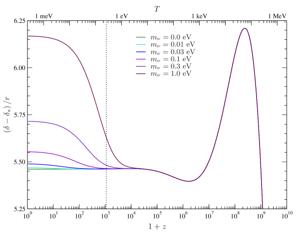
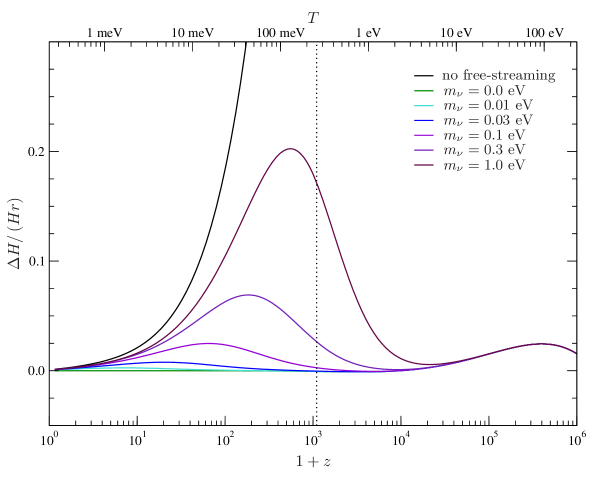
Figure 4: Temperature evolution of $\Delta H/H$ and $\delta-\delta_{\ast}$ for different neutrino masses. We chose the initial conditions to be given by $\delta_{\ast}=0$ at neutrino decoupling. The black solid line in the lower plot represents the temperature evolution of $\Delta H/H$ in the case where only the magnetic field sources the anisotropy and no free-streaming particle is present to compensate this effect. The dotted vertical line indicates the instant of photon decoupling.

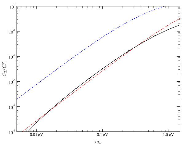
Figure 5: Effect of free-streaming neutrinos with different masses on the quadrupole generated by a homogeneous magnetic field, weighted on the quadrupole obtained without considering the effect of any free-streaming particles. The solid black line represents the result of the numerical integration, the dashed blue and red lines correspond to our analytical prediction given by eq. (47) for two different choices of $t_{m}$, the time at which neutrinos are effectively non-relativistic (see the text for clarification).

Our quantitative final result is shown in fig. 5, where we plot the value of the quadrupole generated by a constant magnetic field, rescaled by $r^{2}$, as function of the neutrino mass. We weight the final $C_{2}$ with respect to the quadrupole obtained without considering the isotropization induced by free-streaming particles, in order to underline the relative importance of this effect. These results clearly show that the CMB quadrupole is significantly reduced by neutrino free-streaming only if their mass is smaller than the temperature at photon decoupling, $m_{\nu}<T_{\rm dec}\simeq 0.26\>\mathrm{eV}$. In fact, for neutrino masses in the range $0.3\>\mathrm{eV}\lesssim m_{\nu}\lesssim 3\>\mathrm{eV}$, the quadrupole $C_{2}$ is reduced by less than a factor $100$ from the result without a free-streaming component, whereas for $0\lesssim m_{\nu}\lesssim 0.3\>\mathrm{eV}$, it decreases by several orders of magnitude. Note, however, that the effect is not negligible even in the former case with relatively large neutrino masses. Fig. 5 also shows our analytical estimation for the final amplitude of the CMB quadrupole produced by this effect as given by eq. (47). Of course the value of eq. (47) depends on the time at which neutrinos become effectively non-relativistic, $t_{m}$. Once we choose $t_{m}$ to be given by the time at which $T=m_{\nu}$, we overestimate the final quadrupole amplitude still by one order of magnitude (dashed blue line). This is a consequence of the fact that the neutrino distribution function is highly relativistic and therefore it takes a further redshift for them to start behaving effectively as massive pressureless particles. This has been considered in the more elaborate estimate given by the dashed red line where we fix the time $t_{m}$ to be given by the time at which $d^{3}P_{\nu}/d(\ln T)^{3}=0$, i.e. the time at which the pressure reaches the break in the power law. This is in excellent agreement with the numerical results.

4 A gravitational wave background and other massless free-streaming components in an anisotropic Universe

From our previous discussion it is evident that any massless free-streaming particle species $X$ can isotropize the Bianchi I model with a constant magnetic field, if present with sufficient contribution $\Omega_{X}$ already in the radiation dominated era. This has to be accounted for if we want to estimate the CMB quadrupole induced by a homogeneous magnetic field.

So far we have discussed the standard model neutrinos as an example of such a particle. However, also other massless particles can play this role, for instance gravitons, but also particle species outside of the spectrum of the standard model. Interestingly, the current bounds on the number of relativistic degrees of freedom during nucleosynthesis, often parameterized by the effective number of additional neutrino species $\Delta N_{\nu}$, allow for the possibility that such a species could be sufficiently abundant. The present bound on $N_{\nu}$ from nucleosynthesis is [14]

$$N_{\nu} = 3.2\pm 1.2~{},$$

$$g_{*} = 2+\frac{7N_{\nu}}{4}\left(\frac{4}{11}\right)^{4/3}=3.36+(N_{\nu}-3)\times 0.454$$ (48)

$$= 3.36+(0.2\pm 1.2)\times 0.454\quad\mbox{ at }95\%\mbox{ confidence.}$$

Here we have taken into account that the photon and neutrino temperatures are related by $T_{\nu}=(4/11)^{1/3}T_{\gamma}$ [16]. The effective $g_{*}$ from $\gamma$ and three species of neutrino corresponds to $g_{*}(\gamma,3\nu)=3.36$. This is equivalent to a limit on an additional relativistic contribution at nucleosynthesis of $\Omega_{X}\lesssim 0.2$. From the solution (38) we know that a free-streaming relativistic species with a density parameter $\Omega_{X}\gtrsim 5/32\simeq 0.156$ during the radiation dominated era will isotropize expansion within a few Hubble times. Since this species will presumably decouple before the neutrinos (otherwise it should have been discovered in laboratory experiments), expansion can be isotropic already at neutrino decoupling, and thus neither the cosmic neutrino background nor the CMB will be affected by anisotropic expansion. In this case therefore, unless we are able to detect the background of the species $X$, we will never find a trace of the anisotropic stress produced by a homogeneous magnetic field. An interesting example are gravitons, which we now want to discuss.

Inflationary models generically predict a background of cosmological gravitational waves which are produced from quantum fluctuations during the inflationary phase. The amplitude of this background, usually expressed by the so-called tensor-to-scalar ratio, $r_{T}$, has not yet been measured, but for a certain class of inflationary models, forthcoming experiments such as Planck might be able to detect these gravitational waves. This is in contrast to the cosmic neutrino background, for which there is no hope of direct detection with current or foreseeable technology. However, this background typically contributes only a very small energy density,

$$\Omega_{\rm GW,\,inf}/\Omega_{\gamma}\simeq 10^{-10}r_{T}~{},\qquad n_{T}\,\raisebox{-2.58334pt}{$\buildrel<\over{\sim}$}\,0\,.$$

Only non-standard inflationary models which allow for $n_{T}>0$ can contribute a significant background, see [18].

Gravitational waves can also be produced during phase transitions in the early Universe [19], after the end of inflation. Such gravitational wave backgrounds can easily contribute the required energy density. Let us therefore concentrate on this possibility.

If the highest energy scales of our Universe remain some orders of magnitude below the Planck scale, gravitational waves are never in thermal equilibrium and can be considered as free-streaming radiation throughout the entire history. Therefore, if the gravitational wave background was statistically isotropic at some very early time, then any amount of anisotropic expansion taking place between this initial time and today will affect the gravitons in a similar fashion as any other free-streaming component, and therefore our present gravitational wave background would be anisotropic. Loosely speaking, the intensity of gravitational waves would be larger in those directions which have experienced less expansion in total since the initial time when the gravitational wave background was isotropic.

As we have specified above, with the current limits on $\Delta N_{\nu}$, the density parameter of gravitons $\Omega_{\mathrm{GW}}$ during nucleosynthesis can be as large as $\sim 0.2$. At higher temperatures (that is, at earlier times), the number of relativistic degrees of freedom increases (more particle species are effectively massless), such that $\Omega_{\mathrm{GW}}$ at earlier time can even be larger. It is therefore conceivable that gravitons acquire sufficient anisotropic stress to compensate the magnetic field and hence take over the role which neutrinos have played in section 3. As already pointed out, in this case, neither neutrinos nor photons will ever experience any significant anisotropic expansion, since the Universe remains in a Friedmann phase after the gravitons have adjusted to the magnetic field. Of course, gravitons remain relativistic for all times and the mass effect which we discussed for the neutrinos does not occur.

In order to rule out this scenario, it would be very interesting not only to measure the background of cosmological gravitational waves but also to determine whether or not it shows a quadrupole anisotropy compatible with such a compensating anisotropic stress. Or in other words: just as the smallness of the CMB quadrupole is a direct indication for isotropic expansion between decoupling of photons and today, the smallness of the quadrupole of a gravitational wave background would inform us about the isotropy of expansion between today and a much earlier epoch where this background was generated.

5 Conclusions

In this paper we have studied a magnetic field coherent over very large scales so that it can be considered homogeneous. We have shown that in the radiation dominated era the well known Bianchi I solution for this geometry is isotropized if a free streaming relativistic component is present and contributes sufficiently to the energy density, $\Omega_{X}\gtrsim 5/32$. This is in tune with the numerical finding [7, 8, 10] that the neutrino anisotropic stresses ‘compensate’ large scale magnetic field stresses. A perturbative explanation of this effect is attempted in [9]. Here we explain the effect for the simple case of a homogeneous magnetic field: free streaming of relativistic particles leads to larger redshift, hence smaller pressure in the directions orthogonal to the field lines where the magnetic field pressure is positive and to smaller redshift, hence larger pressure in the direction parallel to the magnetic field, where the magnetic field pressure is negative. To first order in the difference of the scale factors this effect leads to a build up of anisotropic stress in the free streaming component until it exactly cancels the magnetic field anisotropic stress. This is possible since both these anisotropic stresses scale like $a^{-4}$.

In standard cosmology this free-streaming component is given by neutrinos. However, as soon as neutrinos become massive, their pressure, $P_{\nu}\propto a^{-5}$, decays much faster than their energy density, $\rho_{\nu}\propto a^{-3}$, and the effect of compensation is lost. If this happens significantly after decoupling, there is still a partial cancellation, but if it happens before decoupling, the neutrinos no longer compensate the magnetic field anisotropic stress. Furthermore, a component which starts to free-stream only in the matter era (like e.g. the photons) does not significantly reduce the anisotropic stress. Actually, inserting the dominant part of the constant $D$ from eq. (44) in (42) one finds

$$\frac{\Delta H}{H}=12\Omega_{B}\,,$$ (49)

like without a free-streaming component.

This cancellation of anisotropic stresses does not affect Faraday rotation. A constant magnetic field with amplitude $B_{0}\,\raisebox{-2.58334pt}{$\buildrel>\over{\sim}$}\,10^{-9}$Gauss can therefore be discovered either by the Faraday rotation it induces in the CMB [5], or, if a sufficiently intense gravitational wave background exists, by the quadrupole (anisotropic stress) it generates in it.

Finally, Planck and certainly future large scale structure surveys like Euclid will most probably determine the absolute neutrino mass scale. Once this is known, we can infer exactly by how much the CMB quadrupole from a constant magnetic field is reduced by their presence.

References

-
[1]
P.P. Kronberg, Rept. Prog. Phys. 57, 325 (1994);
T.E. Clarke, P.P. Kronberg and H. Boehringer, Astrophys. J. 547, L111 (2001). -
[2]
C. Caprini and R. Durrer, Phys. Rev. D65, 023517 (2001);
C. Caprini, R. Durrer and E. Fenu, JCAP 0911, 001 (2009). -
[3]
J.D. Barrow, R. Juszkiewicz, and D.H. Sonoda, Mon. Not. R. Astron. Soc. 213, 917 (1985);
J.D. Barrow, Can. J. Phys. 164, 152 (1986);
I.D. Novikov, Sov. Astron. 12, 427 (1968);
A. Kogut, G. Hinshaw, J.D. Barrow, R. Jusciewicz and J. Silk. - [4] J.D. Barrow, P. Ferreira and J. Silk, Phys. Rev. Lett. 78, 3610 (1997).
- [5] E. Scannapieco and P.G. Ferreira Phys. Rev. D.
- [6] E. Komatsu et al. [WMAP Collaboration], Astrophys. J. Supp. 192, 18 (2011) [arXiv:0803.0547].
- [7] D. Paoletti, F. Finelli and F. Paci, Mon. Not. Roy. Astron. Soc. 396, 523 (2009) [arXiv:0811.0230].
- [8] J.R. Shaw, A. Lewis, Phys. Rev. D81, 043517 (2010) [arXiv:0911.2714].
- [9] C. Bonvin and C. Caprini, JCAP 1005:022 (2010) [arXiv:1004.1405].
- [10] K.E. Kunze, Phys. Rev. D83, 023006 (2011) [arXiv:1007.3163].
- [11] P.W. Graham, R. Harnik, and S. Rajendran, Phys. Rev. D82, 063524 (2010) [arXiv:1003.0236].
- [12] R. Durrer, Fund. Cosmic Phys. 15, 209 (1994), [arXiv:astro-ph/9311041].
- [13] A. Pontzen, A. Challinor, Mon. Not. Roy. Astron. Soc. 380, 1387 (2007) [arXiv:0706.2075].
- [14] C. Amsler et al. [Particle Data Group] Phys. Lett. B667, 1 (2008) and 2009 partial update for the 2010 edition..
- [15] D. Larson et al. [WMAP Collaboration], Astrophys. J. Supp. 192, 16 (2011).
- [16] R. Durrer, The Cosmic Microwave background, Cambridge University Press (2008).
- [17] C. Pitrou, Class. Quant. Grav. 26, 065006 (2009).
- [18] R. Camerini, R. Durrer, A. Melchiorri and A. Riotto, Phys. Rev. D77, 101301 (2008) [arXiv:0802.1442].
-
[19]
R. Durrer, Proceedings of the 1st Mediterranean Conference on
Classical and Quantum Gravity (MCCQG).
J. Phys.: Conf. Ser. 222 012021 (2010) [arXiv:1002.1389] ;
C. Caprini, R. Durrer, T. Konstandin, G. Servant, Phys. Rev. D79, 083519 (2009) [arXiv:0901.1661].