Astrometry and photometry with HST WFC3. II. Improved geometric-distortion corrections for 10 filters of the UVIS channel

Abstract

We present an improved geometric-distortion solution for the Hubble Space Telescope UVIS channel of Wide Field Camera 3 for ten broad-band filters. The solution is made up of three parts: (1) a 3^rd-order polynomial to deal with the general optical distortion, (2) a table of residuals that accounts for both chip-related anomalies and fine-structure introduced by the filter, and (3) a linear transformation to put the two chips into a convenient master frame. The final correction is better than 0.008 pixel ($\sim 0.3$ mas) in each coordinate. We provide the solution in two different forms: a FORTRAN subroutine and a set of fits files, one for each filter/chip/coordinate.

1 Introduction, data set, measurements

For various reasons, such as camera optics, alignment errors, filter irregularities, non-flat CCDs, and CCD manufacturing defects, the mapping of the square array of square pixels of a detector onto the tangent-plane projection of the sky requires a non-linear transformation. Positions measured within the pixel grid need to be corrected for geometric distortion (GD) before they can be accurately compared with other positions in the same image, or compared with positions measured in other image.

While almost all scientific programs must make use of the distortion solution, most are relatively insensitive to it. So long as each detector pixel is mapped to within a fraction of a pixel of its true location in a distortion-corrected reference frame, the resampling accuracy is not compromised. For this reason, the formal requirement for distortion calibration for WFC3 was 0.2 pixel to enable MultiDrizzle in the calibration pipeline to generate stacked associations. Kozhurina-Platais et al. (2009; ISR 2009-33) and McClean et al. (2010; ISR 2009-041) have demonstrated that the current official solution is accurate to 0.05 pixel (2 mas), clearly meeting the needs of the pipeline.

Scientific programs that are focused on astrometry make more stringent demands on the distortion solution. These programs must analyze the raw, un-resampled pixels of the distorted images in order to attain the highest possible position accuracy. Similarly, these programs require a more accurate distortion solution to relate measured positions to one another. In general, positions can be measured to a precision of 0.01 pixel for a well-exposed star, so we would like to have a distortion solution that is at least this accurate. Such a precision is well below the formal calibration requirements, but if it can be shown that the solution is stable at that level, then an improved calibration will enable many astrometry-related programs.

In a previous paper (Bellini & Bedin 2009, hereafter Paper I), we used the limited set of dithered exposures taken during SMOV (Servicing Mission Observatory Verification) and an existing ACS/WFC astrometric reference frame as a flat-field to derive a set of 3^rd-order-polynomial correction coefficients to represent the geometric distortion in WFC3/UVIS. The solution was derived independently for each of the two CCDs for each of the three broad-band ultraviolet filters F225W, F275W and F336W.

We found that by applying our correction it was possible to remove the GD over the entire area of each chip to an average 1-D accuracy of 0.025 pixels (i.e., 1 mas). At the time, the lack of sufficient observations collected at different roll angles and dithers prevented a more accurate self-calibration-based solution.

The calibration data collected over the past year has enabled us to undertake the next step in modeling the GD of WFC3/UVIS detectors. The large number of dithers and multiple roll angles now available allow us to construct a 2010-based reference frame that is free of the proper-motion (PM) errors inherent in the previous 2002-epoch ACS catalog. The calibration data has enabled us to extend the GD solution to the rest of the major broad-band filters and to improve the accuracy of the solution to about 0.008 pixel. This is below the precision with which we can measure a well-exposed stars in a single exposure. Improvements beyond this are unlikely, as breathing and other temporal variations make a more accurate “average” solution unnecessary.

As we will see in Sect. 2, the UVIS chips contain distortion with very complex variations on relatively small spatial scales, which would be very unwieldy to model with simple polynomials. Therefore we chose to model the GD with two components: a simple 3^rd-order polynomial and an empirically-derived table of residuals (the look-up table).

These look-up tables (one per chip/filter combination) simultaneously absorb i) the complicated effects caused by the non-perfectly uniform and flat surfaces of the filters (for an example in the case of ACS/WFC, see Anderson & King 2006, hereafter AK06) and ii) the astrometric imprint of manufacturing defects on the UVIS CCD pixel arrays. This approach was pursued with success on both ACS/HRC and ACS/WFC detectors (Anderson 2002, AK06), for which the GD correction based on polynomials plus look-up tables is still the best available to date.

The data used in this paper come from the $\omega$ Cen calibration field, and were collected under programs PID-11452 (PI-Quijano) and PID-11911 (PI-Sabbi) during 4 epochs: 2009 July 15 (2009.54), 2010 January 12–14 (2010.04), 2010 April 28–29 (2010.33) and 2010 June 30–July 4 (2010.51). During the January and April 2010 runs guide-star failures made it necessary to repeat some of the exposures of PID-11911. Moreover, between the first and the second epoch the telescope focus changed significantly. The summary of the observations used in this work is given in Table 1. In addition to large dithers of the size of $\sim$1000 pixels (i.e. $\sim$40^′′), at least 2 orientations were available for each filter.

Star positions and fluxes were obtained as described in Paper I, using a spatially-variable PSF-fitting method, which will be described in detail in a subsequent paper of this series.

Table 1: Log of $\omega$ Cen observations used in this work, sorted by epoch (PID-11452, PID-11911).

Epoch	PA_V3	F225W	F275W	F336W	F390W	F438W
2009.54	$286^{\circ}$		$3\times 350\,$s	$8\times 350\,$s
2010.04	$105^{\circ}$	$9\times 900\,$s	$9\times 800\,$s	$5\times 350\,$s	$8\times 350\,$s	$8\times 350\,$s
2010.33	$200^{\circ}$	$5\times 900\,$s		$1\times 350\,$s	$5\times 350\,$s	$7\times 350\,$s
2010.51	$280^{\circ}$		$9\times 800\,$s	$9\times 350\,$s		$9\times 350\,$s
Epoch	PA_V3	F555W	F606W	F775W	F814W	F850LP
2009.54	$286^{\circ}$
2010.04	$105^{\circ}$	$6\times 40\,$s	$9\times 40\,$s	$9\times 350\,$s	$8\times 40\,$s	$9\times 60\,$s
2010.32	$200^{\circ}$		$9\times 40\,$s(∗)
2010.33	$200^{\circ}$	$9\times 40\,$s	$4\times 40\,$s	$7\times 350\,$s	$6\times 40\,$s	$5\times 60\,$s
2010.51	$280^{\circ}$		$9\times 40\,$s		$9\times 40\,$s
Notes: (∗) used only to derive the meta-coordinate-frame solution (see Sect. 5).

Table 2: Example of coefficients of the 3^rd-order polynomial solution for chip[1] and chip[2] in the case of the F606W filter (coefficients for all the filters are listed in Table A in the electronic version of the paper). Note that the polynomials are normalized such that the size of the coefficient corresponds to the maximum contribution (in pixels) of that term across the chip.

Term $\!(w)\!\!\!\!\!$	Polyn.	$a_{w,[1]}$	$b_{w,[1]}$	$a_{w,[2]}$	$b_{w,[2]}$
1	$\tilde{x}$	$0.000\!$	$\!129.384\!$	$\!0.000\!$	$\!140.280\!$
2	$\tilde{y}$	$0.000\!$	$\!1.868\!$	$\!0.000\!$	$\!-4.251\!$
3	$\tilde{x}^{2}$	$12.044\!$	$\!0.622\!$	$\!11.960\!$	$\!0.762\!$
4	$\tilde{x}\tilde{y}$	$-6.222\!$	$\!5.526\!$	$\!-6.069\!$	$\!5.462\!$
5	$\tilde{y}^{2}$	$0.065\!$	$\!-3.211\!$	$\!0.001\!$	$\!-3.063\!$
6	$\tilde{x}^{3}$	$0.183\!$	$\!0.026\!$	$\!0.096\!$	$\!0.156\!$
7	$\tilde{x}^{2}\tilde{y}$	$-0.054\!$	$\!0.080\!$	$\!0.037\!$	$\!-0.009\!$
8	$\tilde{x}\tilde{y}^{2}$	$0.033\!$	$\!-0.034\!$	$\!0.076\!$	$\!-0.020\!$
9	$\tilde{y}^{3}$	$0.023\!$	$\!-0.009\!$	$\!0.036\!$	$\!0.049\!$

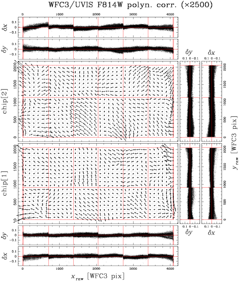
Figure 1: Positional residuals —in the raw-pixel-coordinate system— between the master frame, obtained modeling the GD with only our 3^rd-order polynomial, and the raw position measured on individual exposures. These residuals are averaged within each cell and displayed as arrow vectors (magnified by a factor of 2500). This figure reveals clear discontinuities that cannot be modeled by polynomials of any reasonable order. These discontinuities are marked with red solid lines, which are used to define edges on the look-up table (see the text for more details).

2 The back-bone third-order polynomial solution

The GD solution was constructed in three stages. We began by treating each chip independently. We first solved for the 3^rd-order polynomial that provides the lion’s share of the correction for each chip. After subtracting this global component of the solution, we were then able to see and model the fine-scale component of the solution, caused by detector and filter irregularities. Finally, with the solution for each chip nailed down, we found the global linear parameters that mapped both chips into a convenient meta-chip reference frame.

In Paper I we derived a 3^rd-order polynomial solution for the GD for filters F225W, F275W and F336W; here our aim in this section is to obtain the polynomial solution for seven other broad-band filters for which suitable observations are available, namely: F390W, F438W, F555W, F606W, F775W, F814W and F850LP.

Whereas in Paper I we had to use an astrometric reference catalog that was taken several years prior in order to extract the GD solution, we can now perform a self-calibration of the GD thanks to the improved number of images at different roll angles offered by the new data set. Self-calibrations can often be more accurate than calibrations that reference a standard field, since stars in standard fields can move due to proper motions and since the brightness range where stars in the catalog are well measured may not correspond to the brightness range where stars in the calibration exposures are well measured. Furthermore, the images may have different crowding issues and measurement qualities from the catalog.

We followed the prescriptions given in Anderson & King (2003) for WFPC2 and subsequently used by the same authors to derive the GD correction for the ACS/HRC (Anderson & King 2004) and for the ACS/WFC (AK06). The same strategy was also used by two of us to calibrate a ground-based instrument (see Bellini & Bedin 2010 for details).

Briefly, we started with the F336W GD-solution of Paper I as first guess to correct star positions for the seven redward of F336W (from F390W to F850LP) and created a master frame for each filter independently. We then performed the iterative procedure described in Paper I to improve the polynomial coefficients. With a better GD solution, we then re-constructed the master frames and repeated the entire process three times. A fourth repetition of the procedure provided negligible improvement. The 3^rd-order polynomial coefficients for all 10 of the broad-band filters are hard-coded in the FORTRAN subroutine available at the website described given in Section 6. As an example, the coefficients for filter F606W are reported in Table 2 (coefficients for all the ten filters are shown in Table A in the electronic version of the paper).

3 The fine-scale geometric-distortion table

The next step in the procedure was to examine the residuals from the polynomial solution. To do this we transformed the master-frame position for each star back into the raw frame of each exposure using a conformal linear transformation and the inverse distortion solution. The residual was then the difference between where the star was observed in the frame $(x_{\rm raw},y_{\rm raw})$ and where it should have been in that frame, according to the master frame. In Figure 1 we plot this residual as a function of raw chip coordinate. Each black dot represents a single star measured in single exposure. We combine all the exposures together to see the overall trends.

Individual residuals were then averaged within small ($\sim$113-pixel size) cells (conveniently defined as described in the next section) and are plotted as arrow vectors (magnified by a factor of 2500). These residuals exhibit a pattern with unexpected abrupt discontinuities (denoted with the solid red lines). We note that while some of the large-scale trends could be partially removed by adopting higher-order polynomials, these discontinuities, which have about the same amplitude as the remaining large-scale trends ($\sim$0.02 pixels), would still remain. These residuals are very similar to those seen in Kozhurina-Platais et al. (2010).

It is interesting to note that these $\sim$0.02 pixel systematic trends are perfectly consistent with the larger-than-expected residual dispersion already noted in Paper I. These fine-scale trends were simply washed out by the large internal motions of the $\omega$ Cen stars ($\sim$0.15 WFC3/UVIS pixel) over the 7-year baseline between the reference-frame observations of GO-9442 in 2002 and the WFC3/UVIS observations of PID-11452 in 2009.

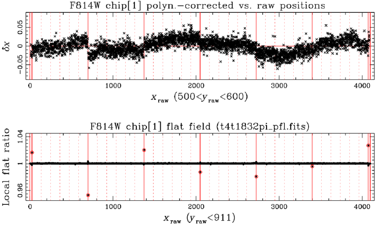
Figure 2: Top: Residuals ($\delta x$) between polynomial-corrected and raw positions plotted against $x_{\rm raw}$ for stars with $500<y_{\rm raw}<600$, in chip[1] for the F814W exposures. Solid lines mark lithographic-pattern discontinuities. Dashed lines show the sampling of our look-up table. The 68.27^th percentile of $\delta x$ for these stars is $\sim$0.02 pixel. It is clear from this figure that uncorrected high-order polynomial residuals and lithographic-pattern residuals have about the same amplitude. Bottom: For each pixel in chip[1] flat field, we took the ratio of the pixel value over the median of the 30 pixel values on either side along $x_{\rm raw}$ directions (independently for each of the two amplifiers). We then took a median of this ratio for all the $y_{\rm raw}<911$ pixels in each column. This is plotted for each of the 4096 columns. It is clear that there are large local flat-field ratio variations at the locations of the lithographic-pattern discontinuities. (highlighted by red open circles), up to $\sim 4$%.

The top panel of Fig. 2 shows the residuals $\delta x$ plotted against the $x_{\rm raw}$ coordinates, for stars measured within a 100-pixel-tall strip, centered at $y_{\rm raw}=550$, extracted from chip[1].

Constraining the $\delta x$ residuals within a vertical strip highlights the sharp changes in the residual trend. It is important to note that these discontinuities are present in both axes of the WFC3/UVIS detectors and not only along a single axis, as was the case for WFPC2 (Anderson & King 1999) or ACS/WFC (Anderson 2002).

The bottom panel of Fig. 2 shows that these boundaries show up as single-row excursions of up to $\sim 4$% in the F814W flat fields. This was also seen for WFPC2 and ACS/WFC.

These discontinuities can be explained as small manufacturing defects in the CCDs, analogous to those found for the WFPC2 and ACS/WFC detectors. These defects arose from an imperfect alignment between the silicon wafer and the mask used to generate the CCDs’ pixel boundaries during lithographic projection (see Kozhurina-Platais et al. 2010). Indeed, at the location where these repositioning errors are found, pixels are wider or narrower in one direction. As a consequence, these pixels are respectively brighter or fainter on the flat field, since they collect more or less light. This also leads to the observed astrometric discontinuities.

The $y_{\rm raw}$-axis pattern of these lithographic features on WFC3/UVIS CCDs are a single pixel wide in the flat field and have a period of 675 pixels along the $x_{\rm raw}$ axis for both chips, extending back and forth from the central position $x_{\rm raw}=2048.5$. Note that this implies that we are left with the first and last 23.5-pixel-wide vertical strips where the discontinuity is repeated. The horizontal feature along the $y_{\rm raw}$ axis consists of a single 2-pixel-wide discontinuity, centered at $y_{\rm raw}=911$ pixels for chip[1] and at $y_{\rm raw}=1140$ pixels for chip[2]. These discontinuities are located symmetrically with respect to the gap between the two chips (horizontal solid red lines in Fig. 1). A careful look at Fig. 2 reveals hints of finer discontinuities on both astrometry (top panel) and flat field (bottom panel), but at much lower amplitudes (a few thousandths of a pixel and $\sim 0.1$%), however it’s hard to assess their significance.

Our aim here was to find a simple correction of the GD following the basic principle: “we see a systematic error, and we empirically find a correction for it”. We therefore decided to keep a polynomial of the third order, as we did in Paper I, to remove most of the GD (down to the $\sim 1$ mas level), and then to use a single look-up table (one for each chip and filter) to correct all the smaller-scale positional systematic errors. This approach was able to provide accuracies down to 0.008 pixel ($\sim 0.3$ mas), as we will show in the next section.

We set up the look-up table as follows. First we defined $x_{\rm raw}$ boundaries alongside the lithographic feature discontinuities (red solid lines in Fig. 1). We subdivided each of the 675-$x_{\rm raw}$-pixel-wide regions into six 112.5-pixel-wide sub-regions, for a total of 36 such subdivisions plus two 23.5-pixel-wide regions at the left and right edges of each chip. To maintain a similar sampling along the $y_{\rm raw}$ axis, we defined 18 sub-divisions. As the horizontal component of the lithographic feature divides the two chips in two parts of 911 and 1140 pixels tall, we made 8 subdivisions for the 911-$y_{\rm raw}$-pixel one (113.875 pixels each) and 10 for the other (114 pixels each). At the end we produced an array of $36\times 18$ almost-square cells, plus two 23.5-pixel-wide strips at the short edges of each chip, each made of 18 rectangular cells (grey dashed lines in Figs. 1).

Cell dimensions were ultimately dictated by the necessity to have enough grid-points to finely sample the GD and to have an adequate number of stars within each cell to robustly measure the value of the grid points in the look-up table. We always had more than 30 stars in each cell to constrain the value of the table, even for the filters with the fewest number of well-exposed stars. Typically we had well over 100 stars per cell.

Figure 3: Example of cell and grid point locations on the detector. This figure shows the bottom-left area of chip[1]. Dotted lines denote those regions used to evaluate the amount of the GD residual at the grid point locations (empty circles). Thick solid lines mark detector edges and dashed lines identify lithographic discontinuities. The arrows illustrate the process of interpolation to evaluate the fine-scale GD residual at a particular location (marked with an $\ast$) using the four closest grid-points. Cell dimensions are also indicated. (See the text for details).

Figure 3 shows an example of the geometry adopted for the look-up tables. Thick solid lines mark detector edges, dashed lines identify lithographic discontinuities, while dotted lines highlight cell borders. We used stars within each cell to compute $3\sigma$-clipped median positional residuals $\overline{\delta x}$ and $\overline{\delta y}$, which are assigned to the corresponding grid point (open circles). When a cell adjoins either detector edges or lithographic discontinuities, the grid point is displaced to the edge of the cell, as shown. We use a semicircle to indicate when a grid point corresponds to a discontinuity.

For any given location on the chip, the look-up table correction is given by a bi-linear interpolation among the surrounding four grid points (as illustrated by the arrows in Fig. 3). In the two 23.5-pixel-wide strips the correction is given by a linear interpolation of the two closest grid points along the $y_{\rm raw}$ axis.

To derive the look-up table we used a master frame which is itself affected by these lithographic features, since it was constructed from positions that had not been corrected for them. Once we had a first estimate of the tabular corrections, we re-determined an improved master frame by correcting our raw catalogs with both the polynomial and the look-up table component. We repeated the whole process of building up master frames and improving the table values three times. A fourth iteration proved to offer negligible improvement.

Figure 4 shows positional residuals in the raw reference system, after our final look-up table plus polynomial GD correction is applied. Residual vectors are now magnified by a factor 100 000. All the lithographic features and all other high-frequency patterns seen on Fig. 1 appear to be completely removed.

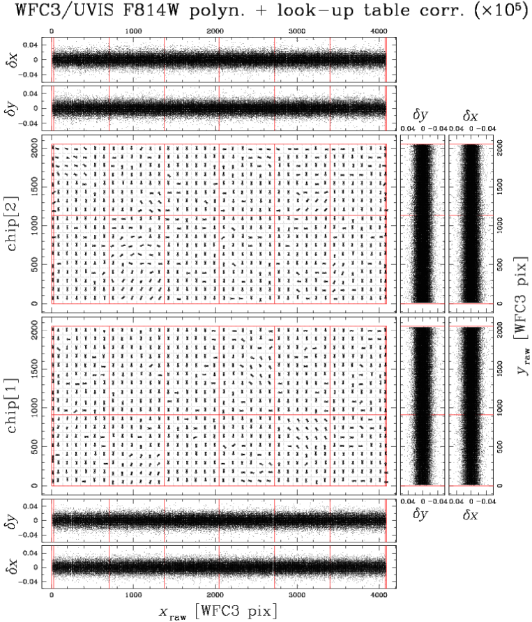
Figure 4: Same as Fig. 1, but after applying the look-up table correction. The size of the residual vectors is now magnified by a factor of $100\,000$. The lithographic pattern has been completely removed.

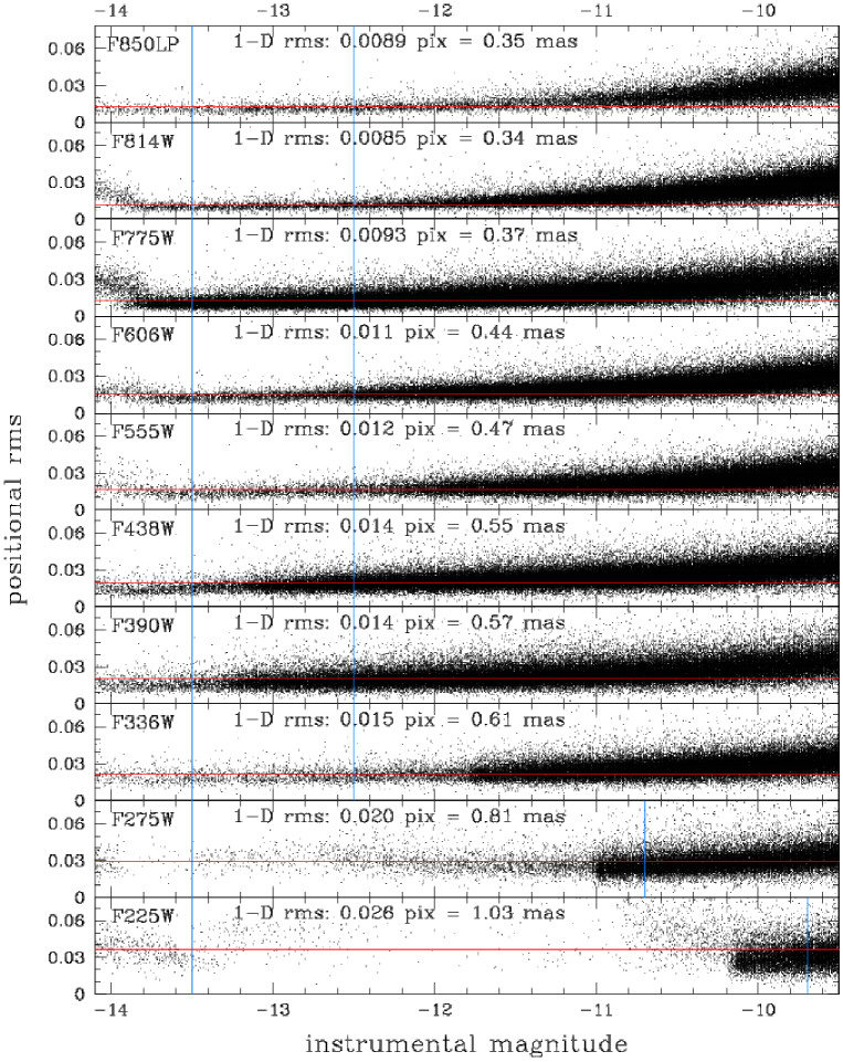
Figure 5: RMS of the positional residuals as a function of instrumental magnitude for each filter. Saturation typically sets in brightward of m${}_{\rm instr.}\sim-13.5$. For well-exposed stars (those within the blue boundaries), we computed the 3$\sigma$-clipped 68.27^th percentile of the positional rms (red lines), for which the 1-D values are reported on top of each panel in units of both WFC3/UVIS pixel and mas.

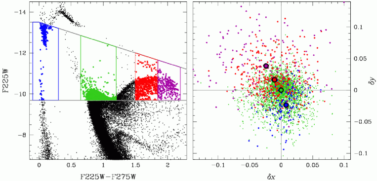
Figure 6: Left: instrumental F225W vs. F225W$-$F275W CMD. We selected only images obtained during the same epoch 2010.04 and transformed the F275W master frame positions into F225W one using only unsaturated stars brighter than F225W$=-9.7$ and with F225W$-$F275W color within 0.65 and 1.2 (in green). We isolated 3 other groups of stars (marked in blue, red and purple). Right: vector-point diagram of the displacements between the two master frames. Stars are color coded in the same way as for the left panel. Full circles mark the median position of each group of stars (median errors have the same size of the circles). There is a clear systematic trend of the displacements as a function of the stars’ color.

One of the best estimates of the true errors of the GD solution is given by the magnitude of the dispersion (computed as the 68.27^th percentile) of the positional residuals (rms) of each star ($i$) observed in each image ($j$), which have been GD-corrected and transformed into the master frame $(x_{{\rm master},i};y_{{\rm master},i})$. These are computed as:

$$\textrm{positional rms${}_{i,j}$ [WFC3/UVIS pixels]}=\sqrt{(x_{i}^{T_{j}}-x_{{\rm master},i})^{2}+(y_{i}^{T_{j}}-y_{{\rm master},i})^{2}}.$$

Only stars observed at least in 3 individual images are used to compute the rms.

Figure 5 shows these dispersions as a function of the corresponding instrumental magnitude for different filters.

Saturation typically sets in brightward of $\sim$$-$13.5 (marked by the left blue vertical line). For well-exposed stars (typically between magnitude $-$13.5 and $-$12.5, but we include fainter stars for F225W and F275W filters to improve the statistics), the 68.27^th percentile levels of the positional rms are marked by red horizontal lines. The corresponding 1-D values are displayed at the top of each panel, in units of both pixels and mas. The best results are obtained for redder filters. Here we used all the images listed in Table 1 (two to four different epochs for each filter) to compute positional rms. We will see in the next section that, by selecting only images within the same epoch, positional dispersions are even smaller.

We noted that very blue and very red stars behave differently with respect to our GD correction when observed through the bluest filters (Kozhurina-Platais et al. (2011) see a similar effect). This is probably due to a chromatic effect induced by fused-silica CCD windows within the optical system, which refract differently blue and red photons and have a sharp increase of the refractive index below 4000 Å (George Hartig, personal communication). As a consequence, the F225W, F275W and F336W filters are the most affected.

To better understand how much astrometry will suffer from this phenomenon, we performed the following test. We chose the F225W and F275W data sets for which the effect is maximized and both extreme horizontal branch (EHB, with a temperature above 40 000 K) and red giant branch (RGB, with a temperature of $\sim$3000 K) stars have about the same luminosity (i.e., our positional dispersions have the same size). We also required images to be taken within the same epoch 2010.04 (9 exposures for each filter), to avoid cluster internal-motion effects.

In the F225W vs. F225W$-$F275W CMD we selected relatively bright (F225W$<$$-$9.7), unsaturated stars of intermediate color (marked in green on the left panel of Fig. 6) and used them to compute a linear transformation from the F275W master frame into the F225W frame. On the same CMD we also selected other groups of stars with the same luminosity criteria: (i) a blue set made up of EHB and hot white-dwarf stars; (ii) a red set containing intermediate RGB stars and (iii) a final purple set populated by RGB-tip stars. Comparing star positional residuals we found that green stars are distributed around (0,0), as we would have expected since their positions formed the basis for the transformations, while stars of the other groups were found to have residuals located in significantly different positions (up to $\sim 0.04$ pixels away). On the right panel of Fig. 6 we show the vector-point diagram for selected stars, which are color coded as on the left panel of the same figure. Median position residuals for each group of stars are marked by full circles of the same colors. The size of the circle indicates the formal error in the median. A systematic trend of the displacements as a function of stellar color is clear. Further investigations will be required to fully characterize this chromatic effect.

4 A demonstrative application

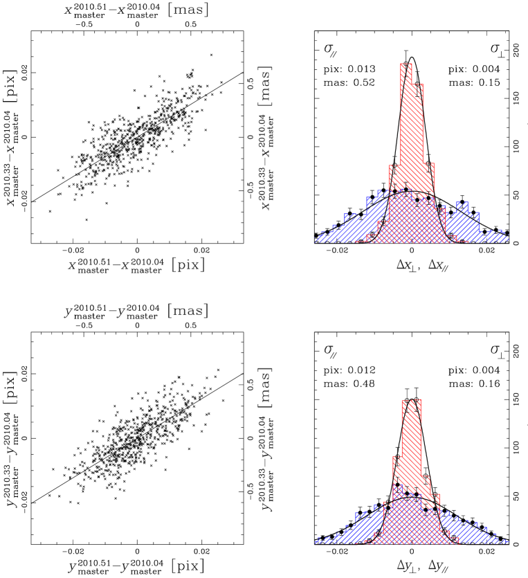
Figure 7: Top-left: correlation between $x$-positional displacements as measured in three different epochs ($E1$, $t_{1}$=2010.04; $E2$, $t_{2}$=2010.33; $E3$, $t_{3}$=2010.51) for the F814W exposures. The slope of the straight line is computed as the the ratio between the two time baselines of $E2-E1$ and $E3-E1$. Top-right: histograms of the displacement distributions along (blue) and perpendicular to (red) the straight line. Bottom panels: the same for $y$-positional displacements. See the text for details.

The globular cluster $\omega$ Cen has the largest internal-proper-motion dispersion among Galactic globular clusters despite being more than two times farther than the closest ones (4.7 kpc, van der Marel & Anderson 2010, versus 2.2 kpc for M 4 and 2.3 kpc for NGC 6397, Harris 1996, Dec. 2010 revision). In this section we show that, by applying our GD solution, we are able to measure this dispersion in just a few months.

To minimize chromatic effects, we used only F814W images and created three distortion-free frames, one for each of the three available epochs ($t_{1}$=2010.04, $t_{2}$=2010.33, $t_{3}$=2010.51, hereafter $E1$, $E2$, $E3$ respectively). We selected well-exposed, unsaturated stars (instrumental magnitude $-13.5<{\rm F814W}<-12.5$) in common to all the three epochs, and compared the positional displacements seen between $(E3-E1)$ and $(E2-E1)$.

Detection of the intrinsic motion of the stars would reveal itself as a correlation between the displacements $(E3-E1)$ and $(E2-E1)$, proportional to the ratio of the respective time baselines $(t_{2}-t_{1})/(t_{3}-t_{1})$. On the contrary, had these displacements been dominated by random errors, we would expect no correlation at all between the two displacements, or at least a correlation with a different slope.

This is shown on the left panels of Fig. 7, where we see a clear correlation between the two coupled epochs in both the $x$- and $y$-directions (top and bottom panels, respectively). Note that the slope of the straight line simply corresponds to the ratio between the two time base-lines and it is not a fit to the data points. If we assume a Gaussian distribution for the observed displacements, the dispersions along the line, and those perpendicular to it, can give us an estimate of the intrinsic proper-motion and the errors’ dispersion, respectively. In the following we will derive a crude estimate for both.

We used the symbols $\sigma_{31}$ and $\sigma_{21}$ [in mas] to indicate the standard deviation of the displacements $(E3-E1)$ and $(E2-E1)$. We then considered that the observed proper-motion dispersion, $\sigma_{\rm obs}$, is related to the intrinsic proper-motion dispersion ($\sigma_{\rm intr}$) and the measurement errors ($\sigma_{\rm err}$) by the following equation:

$$\sigma_{\rm obs}=\sqrt{\sigma_{\rm intr}^{2}+\sigma_{\rm err}^{2}}~{}~{}[\textrm{mas yr}^{-1}].$$

Therefore $\sigma_{\rm intr}$ can be obtained as:

$$\sigma_{\rm intr}=\sqrt{\sigma_{\rm obs}^{2}-\sigma_{\rm err}^{2}}~{}~{}[\textrm{mas yr}^{-1}].$$ (1)

The quantity $\sigma_{\rm obs}$ can also be computed as the ratio between the displacements’ dispersions and their time baseline:

$$\sigma_{\rm obs}=\frac{\sigma_{31}}{t_{3}-t_{1}}=\frac{\sigma_{21}}{t_{2}-t_{1}}~{}~{}[\textrm{mas yr}^{-1}],$$ (2)

from which follows the relation:

$$\sigma_{21}=\frac{t_{2}-t_{1}}{t_{3}-t_{1}}\sigma_{31}~{}~{}[\textrm{mas}].$$

We defined the dispersion of data points along the line in Fig.7 as $\sigma_{\parallel}$, which is an observable quantity and related to the others by the equation

$$\sigma_{\parallel}=\sqrt{\sigma_{31}^{2}+\sigma_{21}^{2}}=\sqrt{\sigma_{31}^{2}+{\frac{(t_{2}-t_{1})^{2}}{(t_{3}-t_{1})^{2}}}\sigma_{31}^{2}}=\sigma_{31}\sqrt{1+{\frac{(t_{2}-t_{1})^{2}}{(t_{3}-t_{1})^{2}}}}~{}~{}[\textrm{mas}],$$

which implies

$$\sigma_{31}=\frac{\sigma_{\parallel}}{\sqrt{1+{\frac{(t_{2}-t_{1})^{2}}{(t_{3}-t_{1})^{2}}}}}~{}~{}[\textrm{mas}].$$

The latter, substituted in Eq. 2, gives

$$\sigma_{\rm obs}=\frac{\sigma_{\parallel}}{(t_{3}-t_{1})\sqrt{1+{\frac{(t_{2}-t_{1})^{2}}{(t_{3}-t_{1})^{2}}}}}~{}~{}{\rm[mas~{}yr^{-1}]},$$ (3)

which relates the observed proper-motion dispersion to the observed dispersion along the expected correlation. Assuming any deviation from the line to represents the total error of the data point, an estimate of $\sigma_{\rm err}$ can be obtained by the dispersion of data points perpendicularly to the line:

$$\sigma_{\rm err}=\frac{\sigma_{\perp}}{(t_{3}-t_{1})\sqrt{1+{\frac{(t_{2}-t_{1})^{2}}{(t_{3}-t_{1})^{2}}}}}~{}~{}{\rm[mas~{}yr^{-1}]},$$ (4)

Top-right panel of Fig. 7 shows the histograms of the $x$-displacement dispersions along (filled circles) and perpendicular (open circles) to the expected correlations. Poisson error bars and Gaussian best fits are also shown. Standard deviations $\sigma_{\parallel}$ and $\sigma_{\perp}$ are computed as the 68.27^th percentile of the distribution residuals around their median value. The bottom-right panel shows the same for $y$-axis displacement dispersions.

Taking the average of $\sigma_{\parallel}$ and $\sigma_{\perp}$ from the displacements along $x$ and $y$, we had $\sigma_{\parallel}\simeq 0.50$ mas and $\sigma_{\perp}\simeq 0.15$ mas. By using the previous equations 1,  3 and 4, we obtained an intrinsic dispersion of $\sigma_{\rm intr}=0.86\pm 0.27$ mas yr^-1, which is in remarkable agreement with the value $\sigma_{\mathrm{1-D}}=0.83\pm 0.07$ mas yr^-1 measured by Anderson & van der Marel (2010) using a time baseline almost 9 times larger (4.07 years vs. 172 days!), and more images. This result is even more astonishing if we consider that we did not use local transformations (see, e.g., Bedin et al. 2003; Anderson et al. 2006, Anderson & van der Marel 2010) which would further reduce systematic residuals in the GD solution, as well as any correction for breathing (which can introduce small low-order terms) or charge-transfer inefficiency (which is already plaguing this new camera; see Figure 8).

As a final external check on the achieved accuracy, we can assume the uncertainties on $E1$ to cancel out and $E2$ and $E3$ to equally contribute to $\sigma_{\perp}$ ($=\sqrt{\sigma_{E2}^{2}+\sigma_{E3}^{2}}=\sqrt{2}\times\sigma_{E}$). Having $\sim$9 exposures per epoch, we can infer a 1-D positional accuracy of 0.008 pixels, $\sim$0.3 mas ($\sqrt{9-1}\times\sigma_{\perp}/\sqrt{2}$), which is consistent with the value reported in Fig. 5. It should also be noted that, at this level of accuracy, there is a considerable interplay between the derived PSF models and the GD solution, which might play some role on the achievable astrometric precision.

Figure 8: A region of $350\times 150$ pixels far from the readout register of a F275W exposure (900 s) obtained in July 2010 (ibc308yeq_flt), where charge-transfer efficiency problems are already visible.

5 Putting the chip-based solution into a global framework.

On account of breathing and other phenomena, the distortion solution is not perfectly stable over time. The impact of breathing is not well enough understood to predict its impact on the distortion, so the best we can hope to achieve is an average distortion solution and a sense of how stable the solution is about this average. It is typically the low-order terms that are the most time-variable, so it made sense above to construct the best single-chip-based solution first and only later to consider the less accurate larger-scale terms that relate the two chips to a common frame. We do that here with the understanding, that for the highest-precision differential astrometry, it is always best to perform the measurements as locally as possible, provided that there are an adequate number of reference stars. Some projects, however have few reference objects and require knowledge of the distortion over the full extent of the field of view (FOV).

We solved for these global terms in several stages. First, we put the two chips into a meta coordinate frame. Next, we solved for the linear skew terms present in the combined system. Then we solved for the overall scaling, so that all filters would have the same scaling, in terms of pixels per arcsecond. Finally, we solved for the positional offset between the filters.

5.1 The Meta Coordinate Frame

We based our meta-coordinate frame on the distortion-corrected frame of the bottom chip (chip[1]). The bottom chip is already in this system, so we simply needed to find the transformation that put the top chip (chip[2]) into this same system. Since there is a gap of about 35 pixels between the frames, the two chips of a single exposure naturally have no sources in common. This means that we will have to use an intermediate set of observations to accomplish the mapping.

We took all the F606W observations and identified all pairs of observations that had either an offset of more than 500 pixels or an orientation difference of more than 10 degrees. (If the pointings are too similar then the overlap will not be sufficient.) Since we wanted as many different pairs of exposures as possible, we also incorporated images from PID-12094 (PI-Kozhurina-Platais), which provides additional roll angles. There were a total of 32 variously overlapping F606W exposures, so in general we could work with 992 overlapping pairs.

For each qualifying pair, we found which chip(s) in the first exposure had significant overlap with both chips in the second exposure. We first corrected all positions for distortion using the solution found above. We next used the positions of common stars to solve for the 4-parameter conformal linear transformation from the top chip of the second exposure into the overlapping chip of the first exposure. We then solved for the analogous transformation from the overlapping chip to the bottom chip of the second exposure. By combining these two linear transformations, we were able to bootstrap positions in the top chip to positions in the bottom chip.

Using all pairs of exposures with good intermediate-chip overlap, we found a transformation of the form:

$$\begin{array}[]{l}xc_{1}=xc_{2}+\Delta x+A\phi_{x}+B\phi_{y}\\ yc_{1}=yc_{2}+\Delta y+C\phi_{x}+D\phi_{y},\end{array}$$ (7)

where $\phi_{x}=(xc_{2}-2048)/4096$ and $\phi_{y}=(yc_{2}-1024)/2048$ to relate the distortion-corrected coordinates in the top chip $(xc_{2},yc_{2})$ into the system of the bottom frame. This was found for each exposure where both of its chips overlapped significantly with a chip from a different exposure.

We then found average values for the six parameters. This gave us a rough meta-frame system. Since the single-chip overlaps can be limited, we then iterated this solution, this time using both chips in the comparison exposure (by means of the meta solution) to examine any residuals in the positioning of the top chip relative to the bottom. We converged upon:

$$\begin{array}[]{l}xc_{1}=xc_{2}-2.020-12.035\phi_{x}-2.367\phi_{y}\\ yc_{1}=yc_{2}+2073.410+2.363\phi_{x}-12.031\phi_{y},\end{array}$$ (10)

for the F606W data set. This means that the central pixel of the top chip (2048,1024), where $\phi_{x}$ and $\phi_{y}$ are zero, is located at coordinate $(2048-2.02,1024+2073.41)$ = $(2045.98,3097.41)$ in the distortion-corrected frame of the bottom chip. The near-conformal nature of this transformation ($A\simeq D$ and $B\simeq-C$) demonstrates that the skew was accurately measured in the original solution.

Now that we had a master frame for the F606W exposures, we used the F606W data set as comparison images to solve for the same parameters for the other filters. We would expect them to be similar, but since the solution for each filter was found independent of the other filters, there could be small scale or orientation changes that would impact the chip[1] frame, and hence the location of chip[2] in chip[1] coordinates. Table 3 provides these inter-chip transformation parameters for all filters.

Table 3: Coefficients used to map the coordinate system of chip[2] into the frame of chip[1] for each filter.

FILT	$\Delta x$	$\Delta y$	$A$	$B$	$C$	$D$	SCALE	DX	DY
F225W	$-$2.024	2073.362	$-$12.152	$-$2.355	2.306	$-$12.146	1.000110	0.200	0.405
F275W	$-$2.001	2073.354	$-$12.123	$-$2.318	2.310	$-$12.116	0.999997	0.265	0.120
F336W	$-$2.023	2073.383	$-$12.068	$-$2.384	2.367	$-$12.068	0.999851	0.440	$-$0.495
F390W	$-$2.001	2073.411	$-$12.098	$-$2.391	2.397	$-$12.110	0.999894	0.280	$-$0.455
F438W	$-$2.003	2073.402	$-$12.097	$-$2.368	2.367	$-$12.096	1.000007	$-$0.075	$-$0.510
F555W	$-$1.996	2073.434	$-$12.063	$-$2.356	2.360	$-$12.046	1.000121	$-$0.085	$-$0.535
F606W	$-$2.020	2073.410	$-$12.035	$-$2.367	2.363	$-$12.031	0.999997	0.000	0.000
F775W	$-$1.975	2073.409	$-$11.995	$-$2.346	2.339	$-$11.987	1.000004	0.260	$-$1.470
F814W	$-$2.048	2073.463	$-$12.038	$-$2.384	2.387	$-$12.033	1.000048	$-$0.070	$-$0.390
F850LP	$-$1.969	2073.389	$-$12.027	$-$2.299	2.300	$-$12.017	1.000158	0.155	$-$0.725

5.2 Solving for the relative scale for each filter.

The solution for each chip/filter combination described above was performed without reference to other chips and filters. The goal of this section is to tie everything together into a common system. In the coordinate transformations above, we always solved for a scale before we examined residuals. The reason for this is that the scale of the telescope is always changing, partly due to breathing and partly due to velocity aberration.

Now that the offset and rotation for each chip/filter combination had been determined to place each of the chips into a common master frame, the overall scale was the last of the linear parameters to be solved for. To do this, we constructed a master frame based on only the F606W exposures using only transformations allowed for offset and rotation, but no scale changes. This way, the frame would represent the average scale of the F606W exposures.

We then transformed the positions of the stars in each of the exposures for each filter (203 in total, including the PID-12094 data) into this reference frame and took note of the scale factor of the linear transformation. We plot this scale factor for each exposure on the top panels of Figure 9. The images are ordered by filter and the filters are separated by a vertical dotted line. It is clear that there is some trend with filter, but there is considerable intra-filter scatter as well. This scatter could be due to velocity aberration or breathing.

Figure 9: Top: The solved-for scale difference between the F606W-based master frame and each individual exposure. The 203 exposures are ordered by filter. The dotted lines correspond to scale changes that would expand the field of view by $\pm$0.01 and $\pm$0.10 pixel. Bottom: The same points, but after velocity aberration has been accounted for.

We divided each of the above scale measurements by the VAFACTOR keyword, taken from the image header. It reports the expected special-relativistic variation in the plate scale, which is related to the dot-product between the average telescope velocity vector during the exposure and the direction to the target (see Cox & Gilliland 2002). After making this deterministic correction, we found that the global exposures for each filter were now consistent to within 0.01 pixel (as shown on the bottom panels of Fig. 9). We solved for the average scaling for each filter and included this correction in the meta distortion solution. The average scaling we found for each filter is given in the eighth column of Table 3. They are in good qualitative agreement with the findings in Figure 2 of Kozhurina-Platais et al. (2010). We note that the linear terms of UVIS appear to be considerably more stable than those of ACS/WFC. Figure 6 of Anderson (2006) shows that the ACS FOV changes in radius by $\pm$0.03 pixel due to breathing, while the residuals here are about 0.01 pixel.

We want emphasize that breathing can introduce errors larger than 0.008 pixel into the distortion solution. Our single-chip-based GD correction was generated comparing largely half-chip to half-chip positions (due to the dithering scheme of the exposures). Therefore, the global effect due to breathing is reduced to about a quarter with respect to what it would be by comparing whole chips to whole chips (since errors tend to be quadratic).

5.3 Solving for the offset for each filter.

Wedge effects can cause individual filters to induce small shifts in the positions of stars on the chip. Since the zeropoint of our distortion solution for each filter is entirely arbitrary, we have the flexibility of choosing it in a convenient way. We would like the distortion solution to have the property that, if a star is observed through two different filters with no dither, the two filters will report the same distortion-corrected position for the star, even if the wedge effect may cause the apparent positions on the chip to differ by more than a pixel.

We identified two sets of consecutive exposures of the $\omega$ Cen central field that had no commanded POS-TARGs between them and found the offset for each filter that best registered its distortion-corrected positions with those of the F606W images. These offsets are given in the last two columns of Table 3. Based on the agreement between the two comparisons we have for each filter, these offsets should be accurate to about 0.05 pixel. Note that the offset for F775W is quite large (1.47 pixel); the others are typically 0.5 pixel.

5.4 The absolute scale.

The distortion solution presented here was constructed to match the pixel scale and orientation of the center of chip[1]. To determine the absolute scale of this frame, we compared the commanded offsets in arcseconds (from the commanded POS_TARGs) with the achieved offsets (in pixels).

PID-11911 contained visits in which 9 exposures in F606W were taken in a 3$\times$3 grid with offsets of 40″ between the exposures. We measured the achieved offsets from the central exposure in distortion-corrected pixels and found that the grid spacing in pixels corresponded to 1005.67 pixels in one visit and 1005.79 in the second visit. This implies a plate scale for our frame of $25.143\pm 0.002$ pixels per arcsecond, which corresponds to $39.773\pm 0.003$ mas pixel^-1. This value is consistent with the independent estimate of the scale given in Paper I ($39.770\pm 0.01$ mas, internal errors only), which is based on the best knowledge of the ACS/WFC absolute scale.

5.5 The final meta frame

After establishing all of these global parameters as described, we noticed that the frame we had adopted, which was centered on the central pixel of chip[1] (the bottom chip), extended into negative coordinates in the lower left of the frame. This is due to our choice of center and the nature of the intrinsic skew present in the detector. Since it is often convenient to work with positive coordinates, we decided to add 200 to the meta coordinate system in $y$, so that positions within the detector would always have positive coordinate values.

6 Conclusions

By using a large number of well dithered data-sets taken with different roll angles, we have modeled the GD of WFC3/UVIS by means of a self-calibration. The solution is an improvement with respect to Paper I and consists of a set of third-order-correction coefficients plus a finely-spaced look-up table of residuals for each chip in 10 filters, namely: F225W, F275W, F336W, F390W, F438W, F555W, F606W, F775W, F814W and F850LP. The hybrid solution has been shown to correct the manufacturing defects and the high-spatial frequency residuals seen in Paper I.

The use of these corrections removes the distortion over the entire area of each chip to an accuracy significantly better than $\sim$0.01 pixel (i.e. better than $\sim$0.4 mas). As a demonstrative test we applied our solution to F814W exposures collected at different epochs and were able to measure the internal motion of $\omega$ Cen in just few months, finding values consistent with the most recent determinations.

The initial solution was constructed for each chip for each filter independently. This is because we did not want any possible motion between the chips or large-scale breathing non-linearities to impact our solution. Once we had the solution for each filter and chip, we unified them into a single common coordinate system. We found the linear transformation that took the top chip into the frame of the bottom chip for each filter, we found the relative scalings between the different filters and finally we found the offsets caused by the wedge-effect of each filter.

We make our FORTRAN routine WFC3_UVIS_gc.f publicly available (at the url www.stsci.edu/$\sim$jayander/WFC3UV_GC/) to the astronomical community. It requires 4 quantities in input: the raw positions $x_{\rm raw}$ and $y_{\rm raw}$, the chip number and the filter. In output it produces corrected positions $x_{\rm corr}$ and $y_{\rm corr}$ in the meta-coordinate frame.

In addition to the FORTRAN code, we will also provide the solution in the form of simple fits images. The “image_format” directory of the website above contains forty images, one for each coordinate/chip/filter combination. As an example, the image gc_wfc3uvis_f606w_chip1x.fits is a 4096$\times$2051 real$\ast$4 image with each pixel in the image giving the $x$ coordinate of the distortion-corrected position of that pixel. To distortion-correct decimal pixel locations, the image can simply be interpolated bi-linearly. These images should make our solution accessible for those who use languages other than FORTRAN.

Finally, we want to state clearly to the reader that this is not the official GD calibration. The IDCTAB file, which contains independent polynomial calibrations for the 10 UVIS filters, is installed in STScI’s Calibration Database System and is used for the OPUS pipeline processing of rectified DRZ images (Kozhurina-Platais et al. 2009, 2010). The two solutions were designed for different goals. Ours was constructed with high-precision differential astrometry in mind, while the official solution was more focused on the absolute transformation onto the focal plane.

A. Appendix

Table A lists the polynomial coefficients for all the 10 filters (F225W, F275W and F336W coefficients are from Bellini & Bedin 2009, reported here for completeness).

Table A: Coefficients of the 3rd-order polynomial solution for chip[1] and chip[2] for all the 10 filters.
Term $\!(w)\!\!\!\!\!$	Polyn.	$a_{w,[1]}$	$b_{w,[1]}$	$a_{w,[2]}$	$b_{w,[2]}$	Term $\!(w)\!\!\!\!\!$	Polyn.	$a_{w,[1]}$	$b_{w,[1]}$	$a_{w,[2]}$	$b_{w,[2]}$
		F225W						F275W
1	$\tilde{x}$	$0.000\!$	$\!129.230\!$	$0.000\!$	$\!140.270\!$	1	$\tilde{x}$	$0.000\!$	$\!129.270\!$	$0.000\!$	$\!140.285\!$
2	$\tilde{y}$	$0.000\!$	$\!1.935\!$	$0.000\!$	$\!-4.215\!$	2	$\tilde{y}$	$0.000\!$	$\!1.925\!$	$0.000\!$	$\!-4.221\!$
3	$\tilde{x}^{2}$	$12.120\!$	$\!0.591\!$	$12.021\!$	$\!0.773\!$	3	$\tilde{x}^{2}$	$12.102\!$	$\!0.581\!$	$12.016\!$	$\!0.781\!$
4	$\tilde{x}\tilde{y}$	$-6.279\!$	$\!5.553\!$	$-6.057\!$	$\!5.496\!$	4	$\tilde{x}\tilde{y}$	$-6.284\!$	$\!5.547\!$	$-6.040\!$	$\!5.493\!$
5	$\tilde{y}^{2}$	$0.064\!$	$\!-3.227\!$	$0.001\!$	$\!-3.058\!$	5	$\tilde{y}^{2}$	$0.061\!$	$\!-3.241\!$	$0.001\!$	$\!-3.048\!$
6	$\tilde{x}^{3}$	$0.176\!$	$\!0.029\!$	$0.149\!$	$\!0.156\!$	6	$\tilde{x}^{3}$	$0.178\!$	$\!0.033\!$	$0.144\!$	$\!0.163\!$
7	$\tilde{x}^{2}\tilde{y}$	$-0.057\!$	$\!0.033\!$	$0.022\!$	$\!-0.009\!$	7	$\tilde{x}^{2}\tilde{y}$	$-0.056\!$	$\!0.054\!$	$0.026\!$	$\!0.007\!$
8	$\tilde{x}\tilde{y}^{2}$	$0.004\!$	$\!-0.041\!$	$0.061\!$	$\!-0.026\!$	8	$\tilde{x}\tilde{y}^{2}$	$0.005\!$	$\!-0.041\!$	$0.051\!$	$\!-0.025\!$
9	$\tilde{y}^{3}$	$0.035\!$	$\!-0.023\!$	$0.032\!$	$\!0.028\!$	9	$\tilde{y}^{3}$	$0.033\!$	$\!-0.012\!$	$0.032\!$	$\!0.020\!$
		F336W						F390W
1	$\tilde{x}$	$0.000\!$	$\!129.438\!$	$0.000\!$	$\!140.315\!$	1	$\tilde{x}$	$0.000\!$	$\!129.364\!$	$0.000\!$	$\!140.216\!$
2	$\tilde{y}$	$0.000\!$	$\!1.786\!$	$0.000\!$	$\!-4.322\!$	2	$\tilde{y}$	$0.000\!$	$\!1.866\!$	$0.000\!$	$\!-4.258\!$
3	$\tilde{x}^{2}$	$12.091\!$	$\!0.676\!$	$11.994\!$	$\!0.672\!$	3	$\tilde{x}^{2}$	$12.058\!$	$\!0.664\!$	$11.959\!$	$\!0.720\!$
4	$\tilde{x}\tilde{y}$	$-6.188\!$	$\!5.565\!$	$-6.135\!$	$\!5.476\!$	4	$\tilde{x}\tilde{y}$	$-6.199\!$	$\!5.551\!$	$-6.114\!$	$\!5.472\!$
5	$\tilde{y}^{2}$	$0.065\!$	$\!-3.155\!$	$0.004\!$	$\!-3.152\!$	5	$\tilde{y}^{2}$	$0.067\!$	$\!-3.161\!$	$-0.007\!$	$\!-3.116\!$
6	$\tilde{x}^{3}$	$-0.062\!$	$\!0.004\!$	$-0.151\!$	$\!0.189\!$	6	$\tilde{x}^{3}$	$0.042\!$	$\!0.014\!$	$0.002\!$	$\!0.177\!$
7	$\tilde{x}^{2}\tilde{y}$	$-0.097\!$	$\!0.034\!$	$0.074\!$	$\!-0.027\!$	7	$\tilde{x}^{2}\tilde{y}$	$-0.083\!$	$\!0.026\!$	$0.070\!$	$\!-0.017\!$
8	$\tilde{x}\tilde{y}^{2}$	$0.016\!$	$\!-0.061\!$	$0.040\!$	$\!0.005\!$	8	$\tilde{x}\tilde{y}^{2}$	$0.016\!$	$\!-0.051\!$	$0.074\!$	$\!0.001\!$
9	$\tilde{y}^{3}$	$0.033\!$	$\!0.016\!$	$0.033\!$	$\!0.014\!$	9	$\tilde{y}^{3}$	$0.050\!$	$\!-0.014\!$	$0.055\!$	$\!0.022\!$
		F438W						F555W
1	$\tilde{x}$	$0.000\!$	$\!129.378\!$	$0.000\!$	$\!140.276\!$	1	$\tilde{x}$	$0.000\!$	$\!129.357\!$	$0.000\!$	$\!140.292\!$
2	$\tilde{y}$	$0.000\!$	$\!1.897\!$	$0.000\!$	$\!-4.258\!$	2	$\tilde{y}$	$0.000\!$	$\!1.931\!$	$0.000\!$	$\!-4.185\!$
3	$\tilde{x}^{2}$	$12.035\!$	$\!0.611\!$	$11.974\!$	$\!0.771\!$	3	$\tilde{x}^{2}$	$12.146\!$	$\!0.579\!$	$12.038\!$	$\!0.770\!$
4	$\tilde{x}\tilde{y}$	$-6.234\!$	$\!5.539\!$	$-6.069\!$	$\!5.492\!$	4	$\tilde{x}\tilde{y}$	$-6.226\!$	$\!5.522\!$	$-6.037\!$	$\!5.464\!$
5	$\tilde{y}^{2}$	$0.063\!$	$\!-3.161\!$	$0.002\!$	$\!-3.079\!$	5	$\tilde{y}^{2}$	$0.062\!$	$\!-3.236\!$	$-0.005\!$	$\!-3.034\!$
6	$\tilde{x}^{3}$	$0.116\!$	$\!0.030\!$	$0.061\!$	$\!0.167\!$	6	$\tilde{x}^{3}$	$0.304\!$	$\!0.032\!$	$0.229\!$	$\!0.119\!$
7	$\tilde{x}^{2}\tilde{y}$	$-0.051\!$	$\!0.054\!$	$0.043\!$	$\!0.027\!$	7	$\tilde{x}^{2}\tilde{y}$	$-0.043\!$	$\!0.047\!$	$-0.014\!$	$\!0.015\!$
8	$\tilde{x}\tilde{y}^{2}$	$0.031\!$	$\!-0.033\!$	$0.073\!$	$\!-0.022\!$	8	$\tilde{x}\tilde{y}^{2}$	$0.023\!$	$\!-0.010\!$	$0.054\!$	$\!-0.019\!$
9	$\tilde{y}^{3}$	$0.041\!$	$\!-0.022\!$	$0.056\!$	$\!0.023\!$	9	$\tilde{y}^{3}$	$0.034\!$	$\!0.005\!$	$0.054\!$	$\!0.018\!$
		F606W						F775W
1	$\tilde{x}$	$0.000\!$	$\!129.384\!$	$0.000\!$	$\!140.280\!$	1	$\tilde{x}$	$0.000\!$	$\!129.322\!$	$0.000\!$	$\!140.167\!$
2	$\tilde{y}$	$0.000\!$	$\!1.868\!$	$0.000\!$	$\!-4.251\!$	2	$\tilde{y}$	$0.000\!$	$\!1.946\!$	$0.000\!$	$\!-4.211\!$
3	$\tilde{x}^{2}$	$12.044\!$	$\!0.622\!$	$11.959\!$	$\!0.762\!$	3	$\tilde{x}^{2}$	$12.044\!$	$\!0.593\!$	$12.022\!$	$\!0.780\!$
4	$\tilde{x}\tilde{y}$	$-6.222\!$	$\!5.526\!$	$-6.069\!$	$\!5.462\!$	4	$\tilde{x}\tilde{y}$	$-6.204\!$	$\!5.538\!$	$-6.040\!$	$\!5.530\!$
5	$\tilde{y}^{2}$	$0.065\!$	$\!-3.211\!$	$0.001\!$	$\!-3.063\!$	5	$\tilde{y}^{2}$	$0.062\!$	$\!-3.171\!$	$0.005\!$	$\!-2.986\!$
6	$\tilde{x}^{3}$	$0.183\!$	$\!0.026\!$	$0.096\!$	$\!0.156\!$	6	$\tilde{x}^{3}$	$0.273\!$	$\!0.002\!$	$0.139\!$	$\!0.228\!$
7	$\tilde{x}^{2}\tilde{y}$	$-0.054\!$	$\!0.080\!$	$0.037\!$	$\!0.009\!$	7	$\tilde{x}^{2}\tilde{y}$	$-0.052\!$	$\!0.042\!$	$0.123\!$	$\!0.002\!$
8	$\tilde{x}\tilde{y}^{2}$	$0.033\!$	$\!-0.034\!$	$0.076\!$	$\!-0.020\!$	8	$\tilde{x}\tilde{y}^{2}$	$0.059\!$	$\!0.006\!$	$0.020\!$	$\!0.037\!$
9	$\tilde{y}^{3}$	$0.023\!$	$\!0.009\!$	$0.036\!$	$\!0.049\!$	9	$\tilde{y}^{3}$	$0.075\!$	$\!-0.001\!$	$0.032\!$	$\!-0.010\!$
		F814W						F850L
1	$\tilde{x}$	$0.000\!$	$\!129.365\!$	$0.000\!$	$\!140.168\!$	1	$\tilde{x}$	$0.000\!$	$\!129.318\!$	$0.000\!$	$\!140.299\!$
2	$\tilde{y}$	$0.000\!$	$\!1.897\!$	$0.000\!$	$\!-4.275\!$	2	$\tilde{y}$	$0.000\!$	$\!1.940\!$	$0.000\!$	$\!-4.208\!$
3	$\tilde{x}^{2}$	$12.025\!$	$\!0.618\!$	$12.058\!$	$\!0.765\!$	3	$\tilde{x}^{2}$	$12.051\!$	$\!0.547\!$	$11.981\!$	$\!0.818\!$
4	$\tilde{x}\tilde{y}$	$-6.219\!$	$\!5.516\!$	$-6.084\!$	$\!5.508\!$	4	$\tilde{x}\tilde{y}$	$-6.236\!$	$\!5.522\!$	$-5.985\!$	$\!5.510\!$
5	$\tilde{y}^{2}$	$0.065\!$	$\!-3.190\!$	$0.003\!$	$\!-3.089\!$	5	$\tilde{y}^{2}$	$0.058\!$	$\!-3.243\!$	$-0.002\!$	$\!-2.992\!$
6	$\tilde{x}^{3}$	$0.192\!$	$\!0.037\!$	$0.064\!$	$\!0.201\!$	6	$\tilde{x}^{3}$	$0.292\!$	$\!0.024\!$	$0.194\!$	$\!0.150\!$
7	$\tilde{x}^{2}\tilde{y}$	$-0.054\!$	$\!0.072\!$	$0.091\!$	$\!0.022\!$	7	$\tilde{x}^{2}\tilde{y}$	$-0.046\!$	$\!0.065\!$	$0.024\!$	$\!0.027\!$
8	$\tilde{x}\tilde{y}^{2}$	$0.047\!$	$\!-0.047\!$	$0.073\!$	$\!0.042\!$	8	$\tilde{x}\tilde{y}^{2}$	$0.042\!$	$\!-0.050\!$	$0.066\!$	$\!-0.030\!$
9	$\tilde{y}^{3}$	$0.037\!$	$\!-0.004\!$	$0.027\!$	$\!0.053\!$	9	$\tilde{y}^{3}$	$0.058\!$	$\!0.001\!$	$0.039\!$	$\!0.040\!$

References

- (1) Anderson, J., & King, I. R. 1999, PASP, 111, 1095
- (2) Anderson, J., & King, I. R. 2000, PASP, 112, 1360
- (3) Anderson, J. 2002, The 2002 HST Calibration Workshop: Hubble after the Installation of the ACS and the NICMOS Cooling System, 13
- (4) Anderson, J., & King, I. R. 2003, PASP, 115, 113
- (5) Anderson, J. 2006, The 2005 HST Calibration Workshop: Hubble After the Transition to Two-Gyro Mode, 11
- (6) Anderson, J., & King, I. R. 2004, Instrument Science Report ACS 2004-15, 51 pages, 1
- (7) Anderson, J., & King, I. R. 2006, Instrument Science Report ACS 2006-01, 34 pages, 1, AK06
- (8) Anderson, J., Bedin, L. R., Piotto, G., Yadav, R. S., & Bellini, A. 2006, A&A, 454, 1029
- (9) Anderson, J. 2007, Instrument Science Report ACS 2007-08, 12 pages, 8
- (10) Anderson, J., & van der Marel, R. P. 2010, ApJ, 710, 1032
- (11) Bellini, A., & Bedin, L. R. 2009, PASP, 121, 1419, Paper I
- (12) Bellini, A., & Bedin, L. R. 2010, A&A, 517, A34
- (13) Cox, C., & Gilliland, R. L. 2002, The 2002 HST Calibration Workshop : Hubble after the Installation of the ACS and the NICMOS Cooling System, 58
- (14) Kozhurina et al. 2009, Instrument Science Report WFC3 2009-033, 22 pages, 33
- (15) Kozhurina-Platais, V., Cox, C, Petro, L., Dulude, M., and Mack, J. ”Multi-Wavelength Geometric Distortion Solution for WFC3/UVIS and IR” in Proceedings of the 2010 HST Calibration Workshop, Eds. S. Deustua and C. Oliveira (Baltimore: STScI), in press (2010).
- (16) Harris, W. E. 1996, AJ, 112, 1487
- (17) van der Marel, R. P., & Anderson, J. 2010, ApJ, 710, 1063