Varying-coefficient functional linear regression

Abstract

Functional linear regression analysis aims to model regression relations which include a functional predictor. The analog of the regression parameter vector or matrix in conventional multivariate or multiple-response linear regression models is a regression parameter function in one or two arguments. If, in addition, one has scalar predictors, as is often the case in applications to longitudinal studies, the question arises how to incorporate these into a functional regression model. We study a varying-coefficient approach where the scalar covariates are modeled as additional arguments of the regression parameter function. This extension of the functional linear regression model is analogous to the extension of conventional linear regression models to varying-coefficient models and shares its advantages, such as increased flexibility; however, the details of this extension are more challenging in the functional case. Our methodology combines smoothing methods with regularization by truncation at a finite number of functional principal components. A practical version is developed and is shown to perform better than functional linear regression for longitudinal data. We investigate the asymptotic properties of varying-coefficient functional linear regression and establish consistency properties.

, and

1 Introduction

Functional linear regression analysis is an extension of ordinary regression to the case where predictors include random functions and responses are scalars or functions. This methodology has recently attracted increasing interest due to its inherent applicability in longitudinal data analysis and other areas of modern data analysis. For an excellent introduction, see Ramsay and Silverman (2005). Assuming that predictor process $X$ possesses a square-integrable trajectory (i.e., $X\in L^{2}(\mathcal{S})$, where $\mathcal{S}\subset\mathbb{R}$), commonly considered functional linear regression models include

$$E(Y|X)=\mu_{Y}+\int_{\mathcal{S}}\beta(s)\bigl{(}X(s)-\mu_{X}(s)\bigr{)}\,\mathrm{d}s,$$ (1)

with a scalar response $Y\in\mathbb{R}$, and

$$E(Y(t)|X)=\mu_{Y}(t)+\int_{\mathcal{S}}\beta(s,t)\bigl{(}X(s)-\mu_{X}(s)\bigr{)}\,\mathrm{d}s,$$ (2)

with a functional response $Y\in L^{2}(\mathcal{T})$ and $\mathcal{T}$ being a subset of the real line $\mathbb{R}$, where $\mu_{X}(s)=E(X(s))$, $s\in\mathcal{S}$ and $\mu_{Y}(t)=E(Y(t))$, $t\in\mathcal{T}$ (Ramsay and Dalzell (1991)). In analogy to the classical regression case, estimating equations for the regression function are based on minimizing the deviation

$$\beta^{*}(s,t)=\operatorname{argmin}\limits_{\beta\in L_{2}(\mathcal{S}\times\mathcal{T})}E\biggl{\{}\int_{\mathcal{T}}\biggl{(}Y(t)-\mu_{Y}(t)-\int_{\mathcal{S}}\beta(s,t)[X(s)-\mu_{X}(s)]\,\mathrm{d}s\biggr{)}^{2}\,\mathrm{d}t\biggr{\}},$$

and analogously for (1). To provide a regularized estimator, one approach is to expand $\beta(\cdot,\cdot)$ in terms of the eigenfunctions of the covariance functions of $X$ and $Y$, and to use an appropriately chosen finite number of the resulting functional principal component (FPC) scores of $X$ as predictors; see, for example, Silverman (1996), Ramsay and Silverman (2002; 2005), Besse and Ramsay (1986), Ramsay and Dalzell (1991), Rice and Silverman (1991), James et al. (2000), Cuevas et al. (2002), Cardot et al. (2003), Hall and Horowitz (2007), Cai and Hall (2006), Cardot (2007) and many others.

Advances in modern technology enable us to collect massive amounts of data at fairly low cost. In such settings, one may observe scalar covariates, in addition to functional predictor and response trajectories. For example, when predicting a response such as blood pressure from functional data, one may wish to utilize functional covariates, such as body mass index, and also additional non-functional covariates $Z$, such as the age of a subject. It is often realistic to expect the regression relation to change as an additional covariate such as age varies. To broaden the applicability of functional linear regression models, we propose to generalize models (1) and (2) by allowing the slope function to depend on some additional scalar covariates $Z$. Previous work on varying-coefficient functional regression models, assuming the case of a scalar response and of continuously observed predictor processes, is due to Cardot and Sarda (2008) and recent investigations of the varying-coefficient approach include Fan et al. (2007) and Zhang et al. (2008).

For ease of presentation, we consider the case of a one-dimensional covariate $Z\in\mathcal{Z}\subset\mathbb{R}$, extending (1) and (2) to the varying-coefficient functional linear regression models

$$E(Y|X,Z)=\mu_{Y|Z}+\int_{\mathcal{S}}\beta(Z,s)\bigl{(}X(s)-\mu_{X|Z}(s)\bigr{)}\,\mathrm{d}s$$ (3)

and

$$E(Y(t)|X,Z)=\mu_{Y|Z}(t)+\int_{\mathcal{S}}\beta(Z,s,t)\bigl{(}X(s)-\mu_{X|Z}(s)\bigr{)}\,\mathrm{d}s\vspace{-2pt}$$ (4)

for scalar and functional responses, respectively, with corresponding characterizations for the regression parameter functions

$$\beta^{*}(z,s) = \mathop{\operatorname{argmin}}_{\beta(z,\cdot)\in L_{2}(\mathcal{S})}E\biggl{\{}\biggl{(}Y-\mu_{Y|Z}-\int_{\mathcal{S}}\beta(Z,s)[X(s)-\mu_{X|Z}(s)]\,\mathrm{d}s\biggr{)}^{2}\Bigm{|}Z=z\biggr{\}},$$

$$\beta^{*}(z,s,t) = \mathop{\operatorname{argmin}}_{\beta(z,\cdot,\cdot)\in L_{2}(\mathcal{S}\times\mathcal{T})}E\biggl{\{}\int_{\mathcal{T}}\biggl{(}Y(t)-\mu_{Y|Z}(t)$$

$${}\hskip 94.0pt-\int_{\mathcal{S}}\beta(Z,s,t)[X(s)-\mu_{X|Z}(s)]\,\mathrm{d}s\biggr{)}^{2}\,\mathrm{d}t\Bigm{|}{Z=z}\biggr{\}}.$$

Here, $\mu_{X|Z}(s)$ and $\mu_{Y|Z}(t)$ denote the conditional mean function of $X$ and $Y$, given $Z$.

Intuitively, after observing a sample of $n$ observations, $\{X_{i},Y_{i},Z_{i}\}_{i=1}^{n}$, the estimation of the varying slope functions can be achieved using kernel methods, as follows:

$$\tilde{\beta}^{*}(z,s) = \operatorname{argmin}\sum_{i=1}^{n}K_{b}(Z_{i}-z)\biggl{[}Y_{i}-\mu_{Y|Z_{i}}-\int_{\mathcal{S}}\beta(Z_{i},s)[X_{i}(s)-\mu_{X|Z_{i}}(s)]\,\mathrm{d}s\biggr{]}^{2}$$

and

$$\tilde{\beta}^{*}(z,s,t) = \operatorname{argmin}\sum_{i=1}^{n}K_{b}({Z_{i}-z})$$

$${}\hskip 43.0pt\times\int_{\mathcal{T}}\biggl{[}Y_{i}(t)-\mu_{Y|Z_{i}}(t)-\int_{\mathcal{S}}\beta(Z_{i},s,t)[X_{i}(s)-\mu_{X|Z_{i}}(s)]\,\mathrm{d}s\biggr{]}^{2}\,\mathrm{d}t$$

for (3) and (4), respectively, where $K_{b}(z)=K(z/b)/b$ for a kernel function $K(\cdot)$ and a bandwidth $b>0$. The necessary regularization of the slope function is conveniently achieved by truncating the Karhunen–Loève expansion of the covariance function for the predictor process (and the response process, if applicable). To avoid difficult technical issues and enable straightforward and rapid implementation, it is expedient to adopt the two-step estimation scheme proposed and extensively studied by Fan and Zhang (2000).

To this end, we first bin our observations according to the values taken by the additional covariate $Z$ into a partition of $\mathcal{Z}$. For each bin, we obtain the sample covariance functions based on the observations within this bin. Assuming that the covariance functions of the predictor and response processes are continuous in $z$ guarantees that these sample covariance functions converge to the corresponding true covariance functions evaluated at the bin centers as bin width goes to zero and sample size increases. This allows us to estimate the slope function at each bin center consistently, using the technique studied in Yao et al. (2005b), providing initial raw estimates. Next, local linear smoothing (Fan and Gijbels (1996)) is applied to improve estimation efficiency, providing our final estimator of the slope function for any $z\in\mathcal{Z}$.

The remainder of the paper is organized as follows. In Section 2, we introduce basic notation and present our estimation scheme. Asymptotic consistency properties are reported in Section 3. Finite-sample implementation issues are discussed in Section 4, results of simulation studies in Section 5 and real data applications in Section 6, with conclusions in Section 7. Technical proofs and auxiliary results are given in the Appendix.

2 Varying coefficient functional linear regression for sparse and irregular data

To facilitate the presentation, we focus on the case of a functional response, which remains largely unexplored. The case with a scalar response can be handled similarly. We also emphasize the case of sparse and irregularly observed data with errors, due to its relevance in longitudinal studies. The motivation of the varying-coefficient functional regression models (3) and (4) is to borrow strength across subjects, while adequately reflecting the effects of the additional covariate. We impose the following smoothness conditions:

1. [[A0]]

2. The conditional mean and covariance functions of the predictor and response processes depend on $Z$ and are continuous in $Z$, that is, $\mu_{X,z}(s)=E(X(s)|Z=z)$, $\mu_{Y,z}(t)=E(Y(t)|Z=z)$, $G_{X,z}(s_{1},s_{2})=\operatorname{cov}(X(s_{1}),X(s_{2})|Z=z)$, $G_{Y,z}(t_{1},t_{2})=\operatorname{cov}(Y(t_{1}),Y(t_{2})|Z=z)$ and $C_{XY,z}(s,t)=\operatorname{cov}(X(s),Y(t)|Z=z)$ are continuous in $z$ and their respective arguments, and have continuous second order partial derivatives with respect to $z$.

Note that [A0] implies that the conditional mean and covariance functions of predictor and response processes do not change radically in a small neighborhood of $Z=z$. This facilitates the estimation of $\beta(z,s,t)$, using the two-step estimation scheme proposed by Fan and Zhang (2000). While, there, the additional covariate $Z$ is assumed to take values on a grid, in our case, $Z$ is more generally assumed to be continuously distributed. In this case, we assume that the additional variable $Z$ has a compact domain $\mathcal{Z}$ and its density $f_{Z}(z)$ is continuous and bounded away from both zero and infinity.

1. [[A1]]

2. $\mathcal{Z}$ is compact, $f_{Z}(z)\in C^{0}$, $\underline{f_{Z}}=\inf_{z\in\mathcal{Z}}f_{Z}(z)>0$ and $\bar{f_{Z}}=\sup_{z\in\mathcal{Z}}f_{Z}(z)<\infty$.

2.1 Representing predictor and response functions via functional principal components for sparse and irregular data

Suppose that we have observations on $n$ subjects. For each subject $i$, conditional on $Z_{i}=z_{i}$, the square-integrable predictor trajectory $X_{i}$ and response trajectory $Y_{i}$ are unobservable realizations of the smooth random processes $(X,Y|Z=z_{i})$, with unknown mean and covariance functions (condition [A0]). The arguments of $X(\cdot)$ and $Y(\cdot)$ are usually referred to as time. Without loss of generality, their domains $\mathcal{S}$ and $\mathcal{T}$ are assumed to be finite and closed intervals. Adopting the general framework of functional data analysis, we assume, for each $z$, that there exist orthogonal expansions of the covariance functions $G_{X,z}(\cdot,\cdot)$ (resp. $G_{Y,z}(\cdot,\cdot)$) in the $L_{2}$ sense via the eigenfunctions $\psi_{z,m}$ (resp. $\phi_{z,k}$), with non-increasing eigenvalues $\rho_{z,m}$ (resp. $\lambda_{z,k}$), that is, $G_{X,z}(s_{1},s_{2})=\sum_{m=1}^{\infty}\rho_{z,m}\psi_{z,m}(s_{1})\psi_{z,m}(s_{2})$, $G_{Y,z}(t_{1},t_{2})=\sum_{k=1}^{\infty}\lambda_{z,k}\phi_{z,k}(t_{1})\phi_{z,k}(t_{2})$.

Instead of observing the full predictor trajectory $X_{i}$ and response trajectory $Y_{i}$, typical longitudinal data consist of noisy observations that are made at sparse and irregularly spaced locations or time points, providing sparse measurements of predictor and response trajectories that are contaminated with additional measurement errors (Staniswalis and Lee (1998), Rice and Wu (2001), Yao et al. (2005a; 2005b)). To adequately reflect the situation of sparse, irregular and possibly subject-specific time points underlying these measurements, we assume that a random number $L_{i}$ (resp. $N_{i}$) of measurements for $X_{i}$ (resp. $Y_{i}$) is made, at times denoted by $S_{i1},S_{i2},\dots,S_{iL_{i}}$ (resp. $T_{i1},T_{i2},\dots,T_{iN_{i}}$). Independent of any other random variables, the numbers of points sampled from each trajectory correspond to random variables $L_{i}$ and $N_{i}$ that are assumed to be i.i.d. as $L$ and $N$ (which may be correlated), respectively. For $1\leq i\leq n$, $1\leq l\leq L_{i}$, $1\leq j\leq N_{i}$, let $U_{il}$ (resp. $V_{ij}$) be the observation of the random trajectory $X_{i}$ (resp. $Y_{i}$) made at a random time $S_{il}$ (resp. $T_{ij}$), contaminated with measurement errors $\varepsilon_{il}$ (resp. $\epsilon_{ij}$). Here, the random measurement errors $\varepsilon_{il}$ and $\epsilon_{ij}$ are assumed to be i.i.d., with mean zero and variances $\sigma_{X}^{2}$ and $\sigma_{Y}^{2}$, respectively. They are independent of all other random variables. The following two assumptions are made.

1. [[A2]]

2. For each subject $i$, $L_{i}\stackrel{{\scriptstyle\mathrm{i.i.d.}}}{{\sim}}L$ (resp. $N_{i}\stackrel{{\scriptstyle\mathrm{i.i.d.}}}{{\sim}}N$) for a positive discrete-valued random variable with $EL<\infty$ (resp. $EN<\infty$) and $P(L>1)>0$ (resp. $P(N>1)>0$).

3. For each subject $i$, observations on $X_{i}$ (resp. $Y_{i}$) are independent of $L_{i}$ (resp. $N_{i}$), that is, $\{(S_{il},U_{il}\colon\ l\in\mathcal{L}_{i})\}$ is independent of $L_{i}$ for any $\mathcal{L}_{i}\subset\{1,2,\ldots,L_{i}\}$ (resp. $\{(T_{ij},V_{ij})\colon\ j\in\mathcal{N}_{i}\}$ is independent of $N_{i}$ for any $\mathcal{N}_{i}\subset\{1,2,\ldots,N_{i}\}$).

It it surprising that under these “longitudinal assumptions”, where the number of observations per subject is fixed and does not increase with sample size, one can nevertheless obtain asymptotic consistency results for the regression relation. This phenomenon was observed in Yao et al. (2005b) and is due to the fact that, according to (7), the target regression function depends only on localized eigenfunctions, localized eigenvalues and cross-covariances of localized functional principal components. However, even though localized, these eigenfunctions and moments can be estimated from pooled data and do not require the fitting of individual trajectories. Even for the case of fitted trajectories, conditional approaches have been implemented successfully, even allowing reasonable derivative estimates to be obtained from very sparse data (Liu and Müller (2009)).

Conditional on $Z_{i}=z$, the FPC scores of $X_{i}$ and $Y_{i}$ are $\zeta_{z,im}=\int[X_{i}(s)-\mu_{X,z}(s)]\psi_{z,m}(s)\,\mathrm{d}s$ and $\xi_{z,ik}=\int[Y_{i}(s)-\mu_{Y,z}(s)]\phi_{z,k}(s)\,\mathrm{d}s,$ respectively. For all $z$, these FPC scores $\zeta_{z,im}$ satisfy $E\zeta_{z,im}=0$, $\operatorname{corr}(\zeta_{z,im_{1}},\zeta_{z,im_{2}})=0$ for any $m_{1}\neq m_{2}$ and $\operatorname{var}(\zeta_{z,im})=\rho_{z,m}$; analogous results hold for $\xi_{z,ik}$. With this notation, using the Karhunen–Loève expansion as in Yao et al. (2005b), conditional on $Z_{i}$, the available measurements of the $i$th predictor and response trajectories can be represented as

$$U_{il} = X_{i}(S_{il})+\varepsilon_{il}$$

$$= \mu_{X,Z_{i}}(S_{il})+\sum_{m=1}^{\infty}\zeta_{Z_{i},im}\psi_{Z_{i},m}(S_{il})+\varepsilon_{il},\qquad 1\leq l\leq L_{i},$$

$$V_{ij} = Y_{i}(T_{ij})+\epsilon_{ij}$$

$$= \mu_{Y,Z_{i}}(T_{ij})+\sum_{k=1}^{\infty}\xi_{Z_{i},ik}\phi_{Z_{i},k}(T_{ij})+\epsilon_{ij},\qquad 1\leq j\leq N_{i}.$$

2.2 Estimation of the slope function

For estimation of the slope function, one standard approach is to expand it in terms of an orthonormal functional basis and to estimate the coefficients of this expansion to estimate the slope function in the non-varying model (2) (Yao et al. (2005b)). As a result of the non-increasing property of the eigenvalues of the covariance functions, such expansions of the slope function are often efficient and require only a few components for a good approximation. Truncation at a finite number of terms provides the necessary regularization. Departing from Yao et al. (2005b), we assume here that an additional covariate $Z$ plays an important role and must be incorporated into the model, motivating (4). To make this model as flexible as possible, the conditional mean and covariance functions of the predictor and response processes are allowed to change smoothly with the value of the covariate $Z$ (Assumption [A0]), which facilitates implementation and analysis of the two-step estimation scheme, as in Fan and Zhang (2000).

Efficient implementation of the two-step estimation scheme begins by binning subjects according to the levels of the additional covariate $Z_{i}$, $i=1,2,\dots,n$. For ease of presentation, we use bins of equal width, although, in practice, non-equidistant bins can occasionally be advantageous. Denoting the bin centers by $z^{(p)},p=1,2,\dots,P$, and the bin width by $h$, the $p$th bin is $[z^{(p)}-\frac{h}{2},z^{(p)}+\frac{h}{2})$ with $h=\frac{\mid\mathcal{Z}\mid}{P}$, where $|\mathcal{Z}|$ denotes the size of the domain of $Z$, $z^{(1)}-h/2\equiv\inf\{z\colon\ z\in\mathcal{Z}\}$ and $z^{(P)}+h/2\equiv\sup\{z\colon\ z\in\mathcal{Z}\}$ (note that the last bin is $[z^{(P)}-h/2,z^{(P)}+h/2]$). Let $\mathcal{N}_{z,h}=\{i\colon\ Z_{i}\in[z-\frac{h}{2},z+\frac{h}{2})\}$ be the index set of those subjects falling into bin $[z-\frac{h}{2},z+\frac{h}{2})$ and $n_{z,h}=\#\mathcal{N}_{z,h}$ the number of those subjects.

2.2.1 Raw estimates

For each bin $[z^{(p)}-\frac{h}{2},z^{(p)}+\frac{h}{2})$, we use the Yao et al. (2005a) method to obtain our raw estimates $\tilde{\mu}_{X,z^{(p)}}(\cdot)$ and $\tilde{\mu}_{Y,z^{(p)}}(\cdot)$ of the conditional mean trajectories and the raw slope function estimate $\tilde{\beta}(z^{(p)},s,t)$. The corresponding raw estimates of $\sigma_{X}^{2}$ and $\sigma_{Y}^{2}$ are denoted by $\tilde{\sigma}_{X,z^{(p)}}^{2}$ and $\tilde{\sigma}_{Y,z^{(p)}}^{2}$ for $p=1,2,\dots,P$. For each $1\leq p\leq P$, the local linear scatterplot smoother of $\tilde{\mu}_{X,z^{(p)}}(s)$ is defined through minimizing

$$\sum_{i\in\mathcal{N}_{z^{(p)},h}}\sum_{j=1}^{N_{i}}\kappa_{1}\biggl{(}\frac{S_{ij}-s}{b_{X,z^{(p)}}}\biggr{)}\bigl{(}U_{ij}-d_{0}-d_{1}(S_{ij}-s)\bigr{)}^{2}$$

with respect to $d_{0}$ and $d_{1}$, and setting $\tilde{\mu}_{X,z^{(p)}}(s)$ to be the minimizer $\hat{d}_{0}$, where $\kappa_{1}(\cdot)$ is a kernel function and $b_{X,z^{(p)}}$ is the smoothing bandwidth, the choice of which will be discussed in Section 4. We define a similar local linear scatterplot smoother of $\tilde{\mu}_{Y,z^{(p)}}(t)$. According to Lemma 3 in the Appendix, raw estimates $\tilde{\mu}_{X,z^{(p)}}(s)$ and $\tilde{\mu}_{Y,z^{(p)}}(t)$ are consistent uniformly for $z^{(p)}$, $p=1,2,\dots,P$, for appropriate bandwidths $b_{X,z^{(p)}}$ and $b_{Y,z^{(p)}}$.

Extending Yao et al. (2005b), the conditional slope function can be represented as

$$\beta(z,s,t)=\sum_{k=1}^{\infty}\sum_{m=1}^{\infty}\frac{E\zeta_{z,m}\xi_{z,k}}{E\zeta_{z,m}^{2}}\psi_{z,m}(s)\phi_{z,k}(t)$$ (7)

for each $z$, where $\psi_{z,m}(\cdot)$ and $\phi_{z,k}(\cdot)$ are the eigenfunctions of covariance functions $G_{X,z}(\cdot,\cdot)$ and $G_{Y,z}(\cdot,\cdot)$, respectively, and $\zeta_{z,m}$ and $\xi_{z,k}$ are the functional principal component scores of $X$ and $Y$, respectively, conditional on $Z=z$.

To obtain raw slope estimates $\tilde{\beta}(z^{(p)},s,t)$ for $p=1,2,\dots,P$, we first estimate the conditional covariance functions $G_{X,z^{(p)}}(s_{1},s_{2})$, $G_{Y,z^{(p)}}(t_{1},t_{2})$ and $C_{XY,z^{(p)}}(s,t)$ at each bin center, based on the observations falling into the bin, using the approach of Yao et al. (2005b). From “raw” covariances, $G_{X,i,z^{(p)}}(S_{ij},S_{ik})=(U_{ij}-\tilde{\mu}_{X,z^{(p)}}(S_{ij}))(U_{ik}-\tilde{\mu}_{X,z^{(p)}}(S_{ik}))$ for $1\leq j,k\leq L_{i}$, $i\in\mathcal{N}_{z^{(p)},h}$ and $p=1,2,\dots,P$, and the locally smoothed conditional covariance $\tilde{G}_{X,z^{(p)}}(s_{1},s_{2})$ is defined as the minimizer $\hat{b}_{0}$ of the local linear problem

$$\min_{b_{0},b_{11},b_{12}}\sum_{i\in\mathcal{N}_{z^{(p)},h}}\sum_{1\leq j\neq l\leq L_{i}}\kappa_{2}\biggl{(}\frac{S_{ij}-s_{1}}{h_{X,z^{(p)}}},\frac{S_{il}-s_{2}}{h_{X,z^{(p)}}}\biggr{)}$$

$${}\hskip 101.0pt\times[G_{X,i,z^{(p)}}(S_{ij},S_{il})-b_{0}-b_{11}(S_{ij}-s_{1})-b_{12}(S_{il}-s_{2})]^{2},$$

where $\kappa_{2}(\cdot,\cdot)$ is a bivariate kernel function and $h_{X,z^{(p)}}$ a smoothing bandwidth. The diagonal “raw” covariances $G_{X,i,z^{(p)}}(S_{ij},S_{ij})$ are removed from the objective function of the above minimization problem because $EG_{X,i,z^{(p)}}(S_{ij},S_{il})\approx\operatorname{cov}(X(S_{ij}),X(S_{il}))+\delta_{jl}\sigma_{X}^{2}$, where $\delta_{jl}=1$ if $j=l$ and $0$ otherwise. Analogous considerations apply for $\tilde{G}_{Y,z^{(p)}}(T_{ij},T_{il})$. The diagonal “raw” covariances $G_{X,i,z^{(p)}}(S_{ij},S_{ij})$ and $G_{Y,i,z^{(p)}}(T_{ij},T_{ij})$ can be smoothed with bandwidths $b_{X,z^{(p)},V}$ and $b_{Y,z^{(p)},V}$, respectively, to estimate $V_{X,z^{(p)}}(s)=G_{X,z^{(p)}}(s,s)+\sigma_{X}^{2}$ and $V_{Y,z^{(p)}}(t)=G_{Y,z^{(p)}}(t,t)+\sigma_{Y}^{2}$, respectively. The resulting estimators are denoted by $\tilde{V}_{X,z^{(p)}}(s)$ and $\tilde{V}_{Y,z^{(p)}}(t)$, respectively, and the differences $(\tilde{V}_{X,z^{(p)}}(s)-\tilde{G}_{X,z^{(p)}}(s,s))$ (and analogously for $Y$) can be used to obtain estimates $\tilde{\sigma}_{X,z^{(p)}}^{2}$ for $\sigma_{X}^{2}$ and $\tilde{\sigma}_{Y,z^{(p)}}^{2}$ for $\sigma_{Y}^{2}$, by integration. Furthermore, “raw” conditional cross-covariances $C_{i,z^{(p)}}(S_{il},T_{ij})=(U_{il}-\tilde{\mu}_{X,z^{(p)}}(S_{il}))(V_{ij}-\tilde{\mu}_{Y,z^{(p)}}(T_{ij}))$ are used to estimate $C_{XY,z^{(p)}}(s,t),$ by minimizing

$$\sum_{i\in\mathcal{N}_{z^{(p)},h}}\sum_{1\leq l\leq L_{i}}\sum_{1\leq j\leq N_{i}}\kappa_{2}\biggl{(}\frac{S_{ij}-s}{h_{1,z^{(p)}}},\frac{T_{ij}-t}{h_{2,z^{(p)}}}\biggr{)}$$

$${}\hskip 88.0pt\times[C_{i,z^{(p)}}(S_{il},T_{ij})-b_{0}-b_{11}(S_{il}-s)-b_{12}(T_{ij}-t)]^{2}$$

with respect to $b_{0}$, $b_{11}$ and $b_{12},$ and setting $\tilde{C}_{XY,z^{(p)}}(s,t)$ to be the minimizer $\hat{b}_{0}$, with smoothing bandwidths $h_{1,z^{(p)}}$ and $h_{2,z^{(p)}}$.

In (7), the slope function may be represented via the eigenvalues and eigenfunctions of the covariance operators. To obtain the estimates $\tilde{\rho}_{z^{(p)},m}$ and $\tilde{\psi}_{z^{(p)},m}(\cdot)$ (resp. $\tilde{\lambda}_{z^{(p)},k}$ and $\tilde{\phi}_{z^{(p)},k}(\cdot)$) of eigenvalue–eigenfunction pairs $\rho_{z^{(p)},m}$ and $\psi_{z^{(p)},m}(\cdot)$ (resp. $\lambda_{z^{(p)},k}$ and $\phi_{z^{(p)},k}(\cdot)$), we use conditional functional principal component analysis (CFPCA) for $\tilde{G}_{X,z^{(p)}}(\cdot,\cdot)$ (resp. $\tilde{G}_{Y,z^{(p)}}(\cdot,\cdot)$), by numerically solving the conditional eigenequations

$$\int_{\mathcal{S}}\tilde{G}_{X,z^{(p)}}(s_{1},s_{2})\tilde{\psi}_{z^{(p)},m}(s_{1})\,\mathrm{d}s_{1} = \tilde{\rho}_{z^{(p)},m}\tilde{\psi}_{z^{(p)},m}(s_{2}),\qquad m=1,2,\ldots,$$ (8)

$$\int_{\mathcal{T}}\tilde{G}_{Y,z^{(p)}}(t_{1},t_{2})\tilde{\phi}_{z^{(p)},k}(t_{1})\,\mathrm{d}t_{1} = \tilde{\lambda}_{z^{(p)},k}\tilde{\phi}_{z^{(p)},k}(t_{2}),\qquad k=1,2,\ldots.$$ (9)

Note that we estimate the conditional mean functions and conditional covariance functions over dense grids of $\mathcal{S}$ and $\mathcal{T}$. Numerical integrations like the one on the left-hand side of (8) are done over these dense grids using the trapezoid rule. Note, further, that integrals over individual trajectories are not needed for the regression focus, in that we use conditional expectation to estimate principal component scores, as in (16).

Due to the fact that

$$C_{XY,z}(s,t) = \operatorname{cov}\bigl{(}X(s),Y(t)|Z=z\bigr{)}=\sum_{k=1}^{\infty}\sum_{m=1}^{\infty}{E(\zeta_{z,m}\xi_{z,k})}\psi_{z,m}(s)\phi_{z,k}(t),$$

we then obtain preliminary estimates of $\sigma_{z,mk}=E(\zeta_{z,m}\xi_{z,k})$ at the bin centers $z^{(p)}$, $p=1,2,\dots,P$, by numerical integration,

$$\tilde{\sigma}_{z^{(p)},mk}=\int_{\mathcal{T}}\int_{\mathcal{S}}\tilde{\psi}_{z^{(p)},m}(s)\tilde{C}_{XY,z^{(p)}}(s,t)\tilde{\phi}_{z^{(p)},k}(t)\,\mathrm{d}s\,\mathrm{d}t.$$ (10)

With (7), (8), (9) and (10), the raw estimates of $\beta(z^{(p)},s,t)$ are

$$\tilde{\beta}\bigl{(}z^{(p)},s,t\bigr{)}=\sum_{k=1}^{K}\sum_{m=1}^{M}\frac{\tilde{\sigma}_{z^{(p)},{mk}}}{\tilde{\rho}_{z^{(p)},m}}\tilde{\psi}_{z^{(p)},m}(s)\tilde{\phi}_{z^{(p)},k}(t).$$ (11)

Further details on the “global” case can be found in Yao et al. (2005b).

2.2.2 Refining the raw estimates

We establish in the Appendix that the raw estimates $\tilde{\mu}_{X,z^{(p)}}(s)$, $\tilde{\mu}_{Y,z^{(p)}}(t)$ and $\tilde{\beta}(z^{(p)},s,t)$ are consistent. As has been demonstrated in Fan and Zhang (2000), there are several reasons to refine such raw estimates. For example, the raw estimates are generally not smooth and are based on local observations, hence inefficient. Most importantly, applications require that the function $\beta(z,s,t)$ is available for any $z\in\mathcal{Z}$.

To refine the raw estimates, the classical approach is smoothing, for which we adopt the local polynomial smoother. Defining $\mathbf{c}_{p}=(1,z^{(p)}-z,\dots,(z^{(p)}-z)^{r})^{T}$, $p=1,2,\dots,P$, the local polynomial smoothing weights for estimating the $q$th derivative of an underlying function are

$$\omega_{q,r+1}\bigl{(}z^{(p)},z,b\bigr{)}=q!\mathbf{e}^{T}_{q+1,r+1}(\mathbf{C}^{T}\mathbf{W}\mathbf{C})^{-1}\mathbf{c}_{p}K_{b}\bigl{(}z^{(p)}-z\bigr{)},\qquad p=1,2,\ldots,P,$$

where $\mathbf{C}=(\mathbf{c}_{1},\mathbf{c}_{2},\dots,\mathbf{c}_{P})^{T}$, $\mathbf{W}=\operatorname{diag}(K_{b}(z^{(1)}-z),K_{b}(z^{(2)}-z),\dots,K_{b}(z^{(P)}-z))$ and $\mathbf{e}_{q+1,r+1}=(0,\dots,0,1,0,\dots,0)^{T}$ is a unit vector of length $r+1$ with the $(q+1)$th element being $1$ (see Fan and Gijbels (1996)). Our final estimators are given by

$$\hat{\mu}_{X,z}(s) = \sum_{p=1}^{P}\omega_{0,2}\bigl{(}z^{(p)},z,b\bigr{)}\tilde{\mu}_{X,z^{(p)}}(s),$$

$$\hat{\mu}_{Y,z}(t) = \sum_{p=1}^{P}\omega_{0,2}\bigl{(}z^{(p)},z,b\bigr{)}\tilde{\mu}_{Y,z^{(p)}}(t),$$

$$\hat{\beta}(z,s,t) = \sum_{p=1}^{P}\omega_{0,2}\bigl{(}z^{(p)},z,b\bigr{)}\tilde{\beta}\bigl{(}z^{(p)},s,t\bigr{)}.$$

Due to the assumption that the variance of the measurement error does not depend on the additional covariate, the final estimators of $\sigma_{X}^{2}$ and $\sigma_{Y}^{2}$ can be taken as simple averages,

$$\hat{\sigma}_{X}^{2}=\sum_{p=1}^{P}\tilde{\sigma}_{X,z^{(p)}}^{2}/P\quad\mbox{and}\quad\hat{\sigma}_{Y}^{2}=\sum_{p=1}^{P}\tilde{\sigma}_{Y,z^{(p)}}^{2}/P.$$ (12)

Remark 1.

The localization to $Z=z$, as needed for the proposed varying coefficient model, coupled with the extreme sparseness assumption [A2], which adequately reflects longitudinal designs, is not conducive to obtaining explicit results in terms of convergence rates for the general case. However, by suitably modifying our arguments and coupling them with the rates of convergence provided on page 2891 of Yao et al. (2005b), we can obtain rates if desired. These are the rates given there, which depend on complex intrinsic properties of the underlying processes, provided that the sample size $n$ is everywhere replaced by $nh$, the sample size for each bin.

Remark 2.

In this work, we focus on sparse and irregularly observed longitudinal data. For the case where entire processes are observed without noise and are error-free, one can estimate the localized eigenfunctions at rates of $L^{2}$-convergence of $(n\tilde{h})^{-1/2}$ (see Hall et al. (2006)), where $\tilde{h}$ is the smoothing bandwidth. For the moments of the functional principal components, a smoothing step is not needed. Known results will be adjusted by replacing $n$ with $nh$ when conditioning on a fixed covariate level $Z=z$; see Cai and Hall (2006) and Hall and Horowitz (2007).

3 Asymptotic properties

We establish some key asymptotic consistency properties for the proposed estimators. Detailed technical conditions and proofs can be found in the Appendix.

The observed data set is denoted by $\{Z_{i},(S_{il},U_{il})_{l=1}^{L_{i}},(T_{ij},V_{ij})_{j=1}^{N_{i}}\colon\ i=1,2,\dots,n\}$. We assume that it comes from (2) and satisfies [A0], [A1], [A2] and [A3].

For $\tilde{n}\propto\sqrt{n}$, define the event

$$E_{n}=\{\min n_{z^{(p)},h}>\tilde{n}\},$$ (13)

where $n_{z^{(p)},h}$ is the number of observations in the $p$th bin and $\tilde{n}\propto\sqrt{n}$ means that there exist $c_{0}$ and $C_{0}$ such that $0<c_{0}\leq\tilde{n}/\sqrt{n}\leq C_{0}<\infty$. It is shown in Proposition 1 in the Appendix that $P(E_{n})\rightarrow 1$ as $n\rightarrow\infty$ for $P\propto n^{1/8}$, as specified by condition (xi).

The global consistency of the final mean and slope function estimates follows from the following theorem.

Theorem 1 ((Consistency of time-varying functional regression))

Under conditions [A0], [A1], [A2] and [A3] in Section 2 and conditions [A4], [A5] and (i)–(xi) in the Appendix, on the event $E_{n}$ with $P(E_{n})\rightarrow 1$ as $n\rightarrow\infty$, we have

$$\int_{\mathcal{Z}}\int_{\mathcal{R}}\bigl{(}\hat{\mu}_{W,z}(r)-\mu_{W,z}(r)\bigr{)}^{2}\,\mathrm{d}r\,\mathrm{d}z\stackrel{{\scriptstyle P}}{{\rightarrow}}0\qquad\mbox{for }W=X,\mathcal{R}=\mathcal{S}\mbox{ and }W=Y,\mathcal{R}=\mathcal{T},$$

and

$$\int_{\mathcal{Z}}\int_{\mathcal{T}}\int_{\mathcal{S}}\bigl{(}\hat{\beta}(z,s,t)-\beta(z,s,t)\bigr{)}^{2}\,\mathrm{d}s\,\mathrm{d}t\,\mathrm{d}z\stackrel{{\scriptstyle P}}{{\rightarrow}}0.$$

To study prediction through time-varying functional regression, consider a new predictor process $X^{*}$ with associated covariate $Z^{*}$. The corresponding conditional expected response process $Y^{*}$ and its prediction $\hat{Y}^{*}$ are given by

$$Y^{*}(t) = E(Y(t)|X^{*},Z^{*})$$

$$= \mu_{Y,Z^{*}}(t)+\int_{\mathcal{S}}\beta(Z^{*},s,t)\bigl{(}X^{*}(s)-\mu_{X,Z^{*}}(s)\bigr{)}\,\mathrm{d}s,$$

$$\hat{Y}^{*}(t) = \hat{\mu}_{Y,Z^{*}}(t)+\int_{\mathcal{S}}\hat{\beta}(Z^{*},s,t)\bigl{(}X^{*}(s)-\hat{\mu}_{X,Z^{*}}(s)\bigr{)}\,\mathrm{d}s.$$ (15)

Theorem 2 ((Consistency of prediction))

For a new predictor process $X^{*}$ with associated covariate $Z^{*}$, it holds under the conditions of Theorem 1 that $\int_{\mathcal{T}}(Y^{*}(t)-\hat{Y}^{*}(t))^{2}\,\mathrm{d}t\stackrel{{\scriptstyle P}}{{\rightarrow}}0$, where $Y^{*}(t)$ and $\hat{Y}^{*}(t)$ are given by (3) and (15).

4 Finite-sample implementation

For the finite-sample case, several smoothing parameters need to be chosen. Following Yao et al. (2005a), the leave-one-curve-out cross-validation method can be used to select smoothing parameters $b_{X,z^{(p)}}$, $b_{Y,z^{(p)}}$, $b_{X,z^{(p)},V}$, $b_{Y,z^{(p)},V}$, $h_{X,z^{(p)}}$, $h_{Y,z^{(p)}}$, $h_{1,z^{(p)}}$ and $h_{2,z^{(p)}}$, individually for each bin. Further required choices concern the bin width $h$, the smoothing bandwidth  $b$ and the numbers $M$ and $K$ of included expansion terms in (11). The method of cross-validation could also be used for these additional choices, but this incurs a heavy computational load. A fast alternative is a pseudo-Akaike information criterion (AIC) (or pseudo-Bayesian information criterion (BIC)).

1. [[1]]

2. Choose the number of terms in the truncated double summation representation $\tilde{\beta}(z^{(p)},s,t)$ for $M(n)$ and $K(n)$, using AIC or BIC, as in Yao et al. (2005b).

3. For each bin width $h$, choose the best smoothing bandwidth $b^{*}(h)$ by minimizing AIC or BIC.

4. Choose the bin width $h^{*}$ which minimizes AIC or BIC, while, for each $h$ investigated, we use $b^{*}(h)$ for $b$.

For [1], we will choose $M$ and $K$ simultaneously for all bins, minimizing the conditional penalized pseudo-deviance given by

$$C(K) = \sum_{p=1}^{P}\sum_{i\in\mathcal{N}_{p}}\biggl{\{}\frac{1}{\tilde{\sigma}_{Y,z^{(p)}}^{2}}\tilde{\bolds\epsilon}_{i}^{T}\tilde{\bolds\epsilon}_{i}+{N_{i}}\log(2\uppi)+{N_{i}}\log\tilde{\sigma}_{Y,z^{(p)}}^{2}\biggr{\}}+\mathcal{P},$$

where $\mathcal{P}=2PK$ for AIC and $\mathcal{P}=(\log n)PK$ for BIC, with respect to $K$. Here, for $i\in\mathcal{N}_{p}$, $\tilde{\bolds{\epsilon}}_{i}=\mathbf{V}_{i}-\tilde{\bolds{\mu}}_{Y,z^{(p)},i}-\sum_{k=1}^{K}{\tilde{\xi}}_{z^{(p)},k,i}^{*}\tilde{\bolds{\phi}}_{z^{(p)},k,i}$ with $\tilde{\bolds{\mu}}_{Y,z^{(p)},i}=({\tilde{\mu}}_{Y,z^{(p)}}(T_{i1}),\dots,{\tilde{\mu}}_{Y,z^{(p)}}(T_{iN_{i}}))^{T}$, $\mathbf{V}_{i}=(V_{i1},\dots,V_{iN_{i}})^{T}$, $\tilde{\bolds{\phi}}_{z^{(p)},k,i}=(\tilde{\phi}_{z^{(p)},k}(T_{i1}),\dots,\tilde{\phi}_{z^{(p)},k}(T_{iN_{i}}))^{T}$ and with estimated principal components

$${\tilde{\xi}}_{z^{(p)},k,i}^{*}={\tilde{\lambda}}_{z^{(p)},k}\tilde{\bolds{\phi}}_{z^{(p)},k,i}^{T}{\tilde{\Sigma}}_{Y,z^{(p)},i}^{-1}(\mathbf{V}_{i}-\tilde{\bolds{\mu}}_{Y,z^{(p)},i}),$$ (16)

where $\tilde{\Sigma}_{Y,z^{(p)},i}$ is an $N_{i}$-by-$N_{i}$ matrix whose $(j,k)$-element is $\tilde{G}_{Y,z^{(p)}}(T_{ij},T_{ik})+\tilde{\sigma}^{2}_{Y,z^{(p)}}\delta_{jk}$. Analogous criteria are used for the predictor process $X$, selecting $K$ by minimizing $\operatorname{AIC}(K)$ and $\operatorname{BIC}(K)$. Marginal versions of these criteria are also available.

In step [2], for each bin width $h$, we first select the best smoothing bandwidth $b^{\ast}(h)$ based on AIC or BIC and then select the final bin width $h^{\ast}$ by a second application of AIC or BIC, plugging $b^{\ast}(h)$ into this selection as follows. For a given bin width $h$, define the $P$-by-$P$ smoothing matrix $\mathbf{S}_{0,2}$ whose $(p_{1},p_{2})$th element is $\omega_{0,2}(z^{(p_{1})},z^{(p_{2})},b)$. The effective number of parameters of the smoothing matrix is then the trace of $\mathbf{S}_{0,2}^{T}\mathbf{S}_{0,2}$ (cf. Wahba (1990)). This suggests minimization of

$$\operatorname{AIC}(b|h) = \sum_{i=1}^{n}\biggl{\{}\frac{1}{\hat{\sigma}^{2}_{Y}}\hat{\bolds\epsilon}_{i}^{T}\hat{\bolds\epsilon}_{i}+{N_{i}}\log(2\uppi)+{N_{i}}\log\hat{\sigma}^{2}_{Y}\biggr{\}}+2\operatorname{tr}(\mathbf{S}_{0,2}^{T}\mathbf{S}_{0,2}),$$

leading to $b^{*}(h)$, where

$${\hat{\bolds\epsilon}}_{i}=\mathbf{V}_{i}-{\hat{\bolds{\mu}}}_{Y,z_{i},i}-\sum_{p=1}^{P}\omega_{0,2}\bigl{(}z^{(p)},z_{i},b\bigr{)}\sum_{m,k=1}^{M,K}\frac{{\tilde{\sigma}}_{z^{(p)},mk}}{\tilde{\rho}_{z^{(p)},m}}{\hat{\zeta}}^{*}_{z^{(p)},m,i}{\tilde{\bolds{\phi}}}_{z^{(p)},k,i}$$

with ${\hat{\bolds{\mu}}}_{Y,z_{i},i}=(\hat{\mu}_{Y,z_{i}}(T_{i1}),\ldots,\hat{\mu}_{Y,z_{i}}(T_{iN_{i}}))^{T}$ and estimated principal component scores

$${\hat{\zeta}}_{z^{(p)},m,i}^{*}={\tilde{\rho}}_{z^{(p)},k}{\tilde{\bolds{\psi}}}_{z^{(p)},m,i}^{T}{\tilde{\Sigma}}_{X,z^{(p)},i}^{-1}(\mathbf{U}_{i}-{\hat{\bolds{\mu}}}_{X,z_{i},i}).$$

The definition of pseudo-BIC scores is analogous.

In step [3], to select the bin width $h^{*}$, we minimize

$$\operatorname{AIC}(h,b^{*}(h))=\sum_{i=1}^{n}\biggl{\{}\frac{1}{{\hat{\sigma}}^{2}_{Y}}{\hat{\bolds\epsilon}}_{i}^{T}\hat{\bolds\epsilon}_{i}+{N_{i}}\log(2\uppi)+{N_{i}}\log\hat{\sigma}^{2}_{Y}\biggr{\}}+2MKP,$$

or the analogous BIC score, using $b^{*}(h)$ for each $h$, as determined in the previous step.

5 Simulation study

We compare global functional linear regression and varying-coefficient functional linear regression through simulated examples with a functional response. For the case of a scalar response, the proposed varying-coefficient functional linear regression approach achieves similar performance improvements (results not reported). For the finite-sample case, there are several parameters to be selected (see Section 4). In the simulations, we use pseudo-AIC to select bin width $h$ and pseudo-BIC to select the smoothing bandwidth $b$ and the number of regularization terms $M(n)$ and $K(n)$.

The domains of predictor and response trajectories are chosen as $\mathcal{S}=[0,10]$ and $\mathcal{T}=[0,10]$, respectively. The predictor trajectories $X$ are generated as $X(s)=\mu_{X}(s)+\sum_{m=1}^{3}\zeta_{m}\psi_{m}(s)$ for $s\in\mathcal{S}$, with mean predictor trajectory $\mu_{X}(s)=(s+\sin(s))$, the three eigenfunctions are $\psi_{1}(s)=-\sqrt{\frac{1}{5}}\cos(\uppi s/5)$, $\psi_{2}(s)=\sqrt{\frac{1}{5}}\sin(\uppi s/5)$, $\psi_{3}(s)=-\sqrt{\frac{1}{5}}\cos(2\uppi s/5)$ and their corresponding functional principal components are independently distributed as $\zeta_{1}\sim N(0,2^{2})$, $\zeta_{2}\sim N(0,\sqrt{2}^{2})$, $\zeta_{3}\sim N(0,1^{2})$. The additional covariate $Z$ is uniformly distributed over $[0,1]$. For $z\in[0,1]$, the slope function is linear in $z$, $\beta(z,s,t)=(z+1)(\psi_{1}(s)\psi_{1}(t)+\psi_{2}(s)\psi_{2}(t)+\psi_{3}(s)\psi_{3}(t))$ and the conditional response trajectory is $E(Y(t)|X,Z=z)=\mu_{Y,z}(t)+\int_{0}^{10}\beta(z,s,t)(X(s)-\mu_{X}(s))\,\mathrm{d}s$, where $\mu_{Y,z}(t)=(1+z)(t+\sin(t))$. We consider the following two cases.

Example 1 ((Regular case)).

The first example focuses on the regular case with dense measurement design. Observations on the predictor and response trajectories are made at $s_{j}=(j-1)/3$ for $j=1,2,\ldots,31$ and $t_{j}=(j-1)/3$ for $j=1,2,\ldots,31$, respectively. We assume the measurement errors on both the predictor and response trajectories are distributed as $N(0,1^{2})$, that is, $\sigma_{X}^{2}=1$ and $\sigma_{Y}^{2}=1$.

Example 2 ((Sparse and irregular case)).

In this example, we make a random number of measurements on each trajectory in the training data set, chosen with equal probability from $\{2,3,\ldots,10\}$. We note that, for the same subject, the number of measurements on the predictor and the number of measurements on the response trajectory are independent. For any trajectory, given the number of measurements, the measurement times are uniformly distributed over the corresponding trajectory domain. The measurement error is distributed as $N(0,1^{2})$ for both the predictor and the response trajectories.

In both examples, the training sample size is 400. An independent test set of size 1000 is generated with the predictor and response trajectories fully observed. We compare performance using mean integrated squared prediction error (MISPE)

$$\frac{1}{1000}\sum_{j=1}^{1000}\int_{\mathcal{T}}\biggl{[}E(Y_{j}^{*}(t)|X_{j}^{*},Z_{j}^{*})$$

$${}\hskip 58.0pt-\biggl{(}\hat{\mu}_{Y,Z_{j}^{*}}(t)+\int_{\mathcal{S}}\hat{\beta}(Z_{j}^{*},s,t)\bigl{(}X_{j}^{*}(s)-\hat{\mu}_{X,Z_{j}^{*}}(s)\bigr{)}\,\mathrm{d}s\biggr{)}\biggr{]}^{2}\,\mathrm{d}t\big{/}|{\mathcal{T}}|,$$

analogously for the global functional linear regression, where $(X_{j}^{*},Y_{j}^{*},Z_{j}^{*})$ denotes the data of the $j$th subject in the independent test set. In Table 1, we report the mean and standard deviation (in parentheses) of the MISPE of the global and varying-coefficient functional linear regression over 100 repetitions for each case. This shows that in this simulation setting, the proposed varying-coefficient functional linear regression approach reduces MISPE drastically, compared with the global functional linear regression, both for regular and sparse irregular designs.

To visualize the differences between predicted conditional expected response trajectories, for a small random sample, in both the regular and sparse and irregular design cases, we randomly choose four subjects from the test set with median values of the integrated squared prediction error (ISPE) for the varying-coefficient functional linear regression. The true and predicted conditional expected response trajectories are plotted in Figure 1, where the left four panels correspond to the regular design case and the right four to the sparse irregular case. Clearly, the locally varying method is seen to be superior.

=10.5cm Functional linear Varying-coefficient functional regression linear regression Regular 4.0146 (1.6115) 0.7836 (0.4734) Sparse and irregular 4.0013 (0.8482) 1.0637 (0.3211)

Table 1: Simulation results: mean and standard deviation of MISPE for global and varying-coefficient functional linear regression with a functional response, for both regular and sparse cases

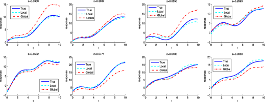
Figure 1: In one random repetition, the true (solid) conditional expected response trajectories and predicted conditional expected response trajectories via the global functional linear regression (dot-dashed) and the varying-coefficient functional linear regression (dashed) are plotted for four randomly selected subjects in the independent test set with median integrated squared prediction error. The left four panels and the right four correspond to the regular and sparse irregular cases, respectively.

6 Applications

We illustrate the comparison of the proposed varying-coefficient functional linear model with the global functional linear regression in two applications.

6.1 Egg-laying data

The egg-laying data represent the entire reproductive history of one thousand Mediterranean fruit flies (‘medflies’ for short), where daily fecundity, quantified by the number of eggs laid per day, was recorded for each fly during its lifetime; see Carey et al. (1998) for details of this data set and experimental background.

We are interested in predicting future egg-laying patterns over an interval of fixed length, but with potentially different starting time, based on the daily fecundity information during a fixed earlier period. The predictor trajectories were chosen as daily fecundity between day 8 and day 17. This interval covers the tail of an initial rapid rise to peak egg-laying and the initial part of the subsequent decline and, generally, the egg-laying behavior at and near peak egg-laying is included. It is of interest to study in what form the intensity of peak egg-laying is associated with subsequent egg-laying behavior, as trade-offs may point to constraints that may play a role in the evolution of longevity.

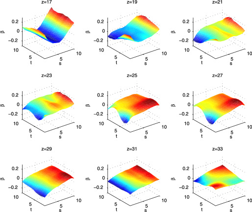
Figure 2: The slope functions estimated by the varying-coefficient functional linear regression at different levels of the additional covariate $z$ for the egg-laying data.

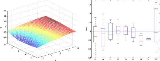
Figure 3: The left panel plots the slope function estimated by the global functional linear regression for the egg-laying data and the right panel corresponds to box plots of the ratios of MSPE of the varying-coefficient functional linear regression to that of the global functional linear regression for the subjects in the test data set for different levels of the additional covariate $Z$.

While the predictor process is chosen with a fixed domain, the response process has a moving domain, with a fixed length of ten days, but a different starting age for each subject, which serves as the additional covariate $Z$. Due to the limited number of subjects in this study, we use a pre-specified discrete set for the values of $Z$: $\mathcal{Z}=\{17,19,21,23,25,27,29,31,33\}$ with a pre-specified bin width $h=2$. For subject $i$ with $z_{i}\in\mathcal{Z}$, measurements $U_{ij}$ on the predictor trajectory are the daily numbers of eggs on day $j+7$, and measurements $V_{ik}$ on the response trajectory correspond to the daily number of eggs on day $k+z_{i}$ for $j=1,2,\dots,10$ and $k=1,2,\dots,10$. The numbers of subjects in these bins are 30, 29, 18, 29, 22, 19, 19, 17 and 36, respectively. For each bin, we randomly select 15 subjects as the training set and the remaining subjects are used to evaluate the prediction performance, comparing the performance of the global and the varying-coefficient functional linear regression. The prediction performance is quantified by mean squared prediction error (MSPE), defined for each subject $i$ in the test set as

$$\operatorname{MSPE}_{g}(i)=\frac{1}{10}\sum_{k=1}^{10}(\hat{y}_{ik}^{g}-V_{ik})^{2}\quad\mbox{and}\quad\operatorname{MSPE}_{l}(i)=\frac{1}{10}\sum_{k=1}^{10}(\hat{y}_{ik}^{l}-V_{ik})^{2},$$

where $\hat{y}_{ik}^{g}$ and $\hat{y}_{ik}^{l}$ denote the predicted daily fecundities corresponding to $V_{ik}$ using the global (resp. the proposed varying-coefficient (local)) functional linear regression.

Through pseudo-AIC, the global functional linear regression selects two and three principal components for the predictor and response trajectories, respectively, while the varying-coefficient functional linear regression uses two principal components for both trajectories. After smoothing, the slope functions estimated by the varying-coefficient models are plotted in Figure 2 for different values of $Z$ and the estimated slope function for the global functional linear regression is plotted in the left panel of Figure 3. Box plots of the ratio $\operatorname{MSPE}_{l}(i)/\operatorname{MSPE}_{g}(i)$ for subjects in the test data set are shown in the right panel of Figure 3 for different levels of the covariate $Z$. There is one outlier above the maximum value for $Z=18$ which is not shown. For most bins, the median ratios are seen to be smaller than 1, indicating an improvement of our new varying-coefficient functional linear regression. Denoting the average MSPE (over the independent test data set) of the global and the varying-coefficient functional linear regression by $\overline{\operatorname{MSPE}}_{g}$ and $\overline{\operatorname{MSPE}}_{l}$, respectively, the relative performance gain $(\overline{\operatorname{MSPE}}_{l}-\overline{\operatorname{MSPE}}_{g})/\overline{\operatorname{MSPE}}_{g}$ is found to be $-0.0810$ so that the prediction improvement of the varying-coefficient method is $8.1\%$.

Besides prediction, it is of interest to study the dependency of the future egg-laying behavior on peak egg-laying. From the changing slope functions in Figure 2, we find that, for the segments close to the peak segments, the egg-laying pattern is inverting the peak pattern, meaning that sharper and higher peaks are associated with sharp downturns, pointing to a near-future exhaustion effect of peak egg-laying. In contrast, the shape of egg-laying segments further into the future is predicted by the behavior of the first derivative over the predictor segment so that slow declines near the end of peak egg-laying are harbingers of future robust egg-laying. This is in accordance with a model of exponential decline in egg-laying that has been proposed by Müller et al. (2001).

6.2 BLSA data with scalar response

As a second example, we use a subset of data from the Baltimore Longitudinal Study of Aging (BLSA), a major longitudinal data set for human aging (Shock et al. (1984), Pearson et al. (1997)). The data consist of 1590 male volunteers who were scheduled to be seen twice per year. However, many participants missed scheduled visits or were seen at other than scheduled times so that the data are sparse and irregular with unequal numbers of measurements and different measurement times for each subject. For each subject, current age and systolic blood pressure (SBP) were recorded during each visit. We quantify how the SBP trajectories of a subject available in a middle age range between age 48 and age 53 affect the average of the SBP measurements made during the last five years included in this study, at an older age. The predictor domain is therefore of length five years and the response is scalar. The additional covariate for each subject is the beginning age of the last five-year interval included in the study. After excluding subjects with less than two measurements in the predictor, 214 subjects were included for whom the additional covariate ranged between 55 and 75. We bin the data according to the additional covariate, with bin centers at ages 56.0, 59.0, 62.0, 65.0, 68.5 and 73.0 years and the numbers of subjects in each of these bins are 38, 33, 38, 32, 39 and 34.

We randomly selected 25 subjects from each bin for model estimation and used the remaining subjects to evaluate the prediction performance. In contrast to the egg-laying data, the predictor measurements in this longitudinal study are sparse and irregular. Pseudo-BIC selects two principal components for the predictor trajectories for both global and varying-coefficient functional linear regressions. Using the same criterion for relative performance gain as in the previous example, the varying-coefficient functional linear regression achieves $11.8\%$ improvement compared to the global functional linear regression. Estimated slope functions are shown in Figure 5 and predictor trajectories in Figure 4.

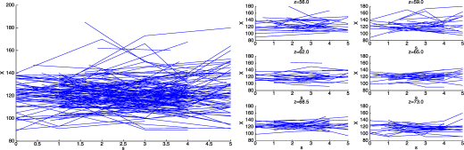
Figure 4: Plots of predictor processes: the left panel for the global functional linear regression and the right panel for different bins according to the additional covariate in the varying-coefficient functional linear regression.

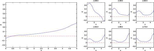
Figure 5: The estimated slope function via the global functional linear regression and the new proposed varying-coefficient functional linear regression (for different levels of $Z$) are plotted as the solid lines in the left and right panels, respectively.

The shape changes of the slope functions with changing covariate indicate that the negative derivative of SBP during the middle-age period is associated with near-future SBP. Further into the future, this pattern is reversed and an SBP increase near the right end of the initial period is becoming predictive.

7 Concluding remarks

Our results indicate that established functional linear regression models can be improved when an available covariate is incorporated. We implement this idea by extending the functional linear model to a varying-coefficient version, inspired by the analogous, highly successful extension of classical regression models. In both application examples, the increased flexibility that is inherent in this extension] leads to clear gains in prediction error. In addition, it is often of interest to ascertain the effect of the additional covariate. This can be done by plotting the regression slopes for each bin defined by the covariate and observing the dependency of this function or surface on the value of the covariate.

Further extensions that are of interest in many applications concern the case of multivariate covariates. If the dimension is low, the smoothing methods and binning methods that we propose here can be extended to this case. For higher-dimensional covariates or covariates that are not continuous, one could form a single index to summarize the covariates and thus create a new one-dimensional covariate which then enters the functional regression model in the same way as the one-dimensional covariate that we consider.

As seen in the data applications, the major applications of the proposed methodology are expected to come from longitudinal studies with sparse and irregular measurements, where the presence of additional non-functional covariates is common.

Appendix: Auxiliary results and proofs

We note that further details, such as omitted proofs, can be found in a technical report that is available at http://www4.stat.ncsu.edu/~wu/WuFanMueller.pdf.

A bivariate kernel function $\kappa_{2}(\cdot,\cdot)$ is said to be of order $(\nu,\ell)$ with $\nu=(\nu_{1},\nu_{2})$ if it satisfies

$$\int u^{\ell_{1}}v^{\ell_{2}}\kappa_{2}(u,v)\,\mathrm{d}u\,\mathrm{d}v=\cases{0,&\quad$0\leq\ell_{1}+\ell_{2}<\ell,\ell_{1}\neq\nu_{1},\ell_{2}\neq\nu_{2},$\cr\nu!,&\quad$\ell_{1}=\nu_{1},\ell_{2}=\nu_{2},$\cr\neq 0,&\quad$\ell_{1}+\ell_{2}=\ell$,}$$ (17)

and

$$\int|u^{\ell_{1}}v^{\ell_{2}}\kappa_{2}(u,v)|\,\mathrm{d}u\,\mathrm{d}v<\infty\qquad\mbox{for any }\ell_{1}+\ell_{2}=\ell,$$ (18)

where $\nu!=\nu_{1}!\cdot\nu_{2}!$. Similarly, a univariate kernel function $\kappa_{1}(\cdot)$ is of order $(\nu,\ell)$ for a univariate $\nu=\nu_{1}$ when (17) and (18) hold for $\ell_{2}\equiv 0$ on the right-hand side while integrating over the univariate argument $u$ on the left.

We introduce the following technical conditions:

1. [(viii)]

2. The variable $S$ has compact domain $\mathcal{S}$. Given $Z=z$, $S$ has conditional density $f_{S,z}(s)$. Assume, uniformly in $z\in\mathcal{Z}$, that $\frac{\partial^{\ell}}{\partial s^{\ell}}f_{S,z}(s)$ exists and is continuous for $\ell=2$ on $\mathcal{S}$ and, further, $\inf_{s\in\mathcal{S}}f_{S,z}(s)>0$, analogously for $T$.

3. Denote the conditional density functions of $(S,U)$ and $(T,V)$ by $g_{X,z}(s,u)$ and $g_{Y,z}(t,v)$, respectively. Assume that the derivative ${\textstyle\frac{\partial^{\ell}}{\partial s^{\ell}}}g_{X,z}(s,u)$ exists for all arguments $(s,u)$, is uniformly continuous on $\mathcal{S}\times\mathbb{R}$ and is Lipschitz continuous in $z$, for $\ell=2$, analogously for $g_{Y,z}(t,v)$.

4. Denote the conditional density functions of quadruples $(S_{1},S_{2},U_{1},U_{2})$ and $(T_{1},T_{2},V_{1},V_{2})$ by $g_{2X,z}(s_{1},s_{2},u_{1},u_{2})$ and $g_{2Y,z}(t_{1},t_{2},v_{1},v_{2})$, respectively. For simplicity, the corresponding marginal conditional densities of $(S_{1},S_{2})$ and $(T_{1},T_{2})$ are also denoted by $g_{2X,z}(s_{1},s_{2})$ and $g_{2Y,z}(t_{1},t_{2})$, respectively. Denote the conditional density of $(S,T,U,V)$ given $Z=z$ by $g_{XY,z}(s,t,u,v)$ and, similarly, its corresponding conditional marginal density of $(S,T)$ by $g_{XY,z}(s,t)$. Assume that the derivatives $\frac{\partial^{\ell}}{\partial s_{1}^{\ell_{1}}\,\partial s_{2}^{\ell_{2}}}g_{2X,z}(s_{1},s_{2},u_{1},u_{2})$ exist for all arguments $(s_{1},s_{2},u_{1},u_{2})$, are uniformly continuous on $\mathcal{S}^{2}\times\mathbb{R}^{2}$ and are Lipschitz continuous in $z$ for $\ell_{1}+\ell_{2}=\ell$, $0\leq\ell_{1},\ell_{2}\leq\ell=2$, analogously for $g_{2Y,z}(t_{1},t_{2},v_{1},v_{2})$ and $g_{XY,z}(s,t,u,v)$.

5. For every $p=1,2,\dots,P$, $b_{X,z^{(p)}}\rightarrow 0$, $n_{z^{(p)},h}b_{X,z^{(p)}}^{4}\rightarrow\infty$, $n_{z^{(p)},h}b_{X,z^{(p)}}^{6}<\infty$, $b_{Y,z^{(p)}}\rightarrow 0$, $n_{z^{(p)},h}b_{Y,z^{(p)}}^{4}\rightarrow\infty$ and $n_{z^{(p)},h}b_{Y,z^{(p)}}^{6}<\infty$ as $n\rightarrow\infty$.

6. For every $p=1,2,\dots,P$, $h_{X,z^{(p)}}\rightarrow 0$, $n_{z^{(p)},h}h_{X,z^{(p)}}^{6}\rightarrow\infty$, $n_{z^{(p)},h}h_{X,z^{(p)}}^{8}<\infty$, $h_{Y,z^{(p)}}\rightarrow 0$, $n_{z^{(p)},h}h_{Y,z^{(p)}}^{6}\rightarrow\infty$ and $n_{z^{(p)},h}h_{Y,z^{(p)}}^{8}<\infty$ as $n\rightarrow\infty$.

7. For every $p=1,2,\dots,P$, $h_{1,z^{(p)}}/h_{2,z^{(p)}}\rightarrow 1$, $h_{1,z^{(p)}}\rightarrow 0$, $n_{z^{(p)},h}h_{1,z^{(p)}}^{6}\rightarrow\infty$ and $n_{z^{(p)},h}h_{1,z^{(p)}}^{8}<\infty$ as $n\rightarrow\infty$.

8. For every $p=1,2,\dots,P$, $b_{X,z^{(p)},V}\rightarrow 0$, $n_{z^{(p)},h}b_{X,z^{(p)},V}^{4}\rightarrow\infty$, $n_{z^{(p)},h}b_{X,z^{(p)},V}^{6}<\infty$, $b_{Y,z^{(p)},V}\rightarrow 0$, $n_{z^{(p)},h}b_{Y,z^{(p)},V}^{4}\rightarrow\infty$ and $n_{z^{(p)},h}b_{Y,z^{(p)},V}^{6}<\infty$ as $n\rightarrow\infty$.

9. Univariate kernel $\kappa_{1}$ and bivariate kernel $\kappa_{2}$ are compactly supported, absolutely integrable and of orders $(\nu,\ell)=(0,2)$ and $((0,0),2)$, respectively.

10. Assume that $\sup_{(z,s)\in\mathcal{Z}\times\mathcal{S}}E(E(X(s)-\mu_{X,Z}(s))^{4}|Z=z))<\infty$, and analogously for $Y$.

11. The slope function $\beta(z,s,t)$ is twice differentiable in $z$, that is, for any $(s,t)\in\mathcal{S}\times\mathcal{T}$, $\frac{\partial^{2}}{\partial z^{2}}\beta(z,s,t)$ exists and is continuous in $z$.

12. The bin width $h$ and smoothing bandwidth $b$ are such that $b/h<\infty$ as $n\rightarrow\infty$. The bin width $h$ is chosen such that $P\propto n^{1/8}$.

Proposition 0.

For $E_{n}$ defined in (13), under (xi), it holds that $P(E_{n})\rightarrow 1$ as $n\rightarrow\infty$.

Proof.

First, note that $P(\min n_{z^{(p)},h}>\tilde{n})\geq 1-\sum_{p=1}^{P}P(n_{z^{(p)},h}<\tilde{n}).$ Consider the $p$th bin and let $\pi_{p}=P(Z\in[z^{(p)}-\frac{h}{2},z^{(p)}-\frac{h}{2}))$. Then $n_{z^{(p)},h}$ is asymptotically distributed as $N(n\pi_{p},n\pi_{p}(1-\pi_{p}))$ due to the normal approximation to a binomial random variable. Thus, $P(n_{z^{(p)},h}>\tilde{n})\rightarrow f_{N(0,1)}(a_{p})/a_{p}$ with $a_{p}=-(\tilde{n}-n\pi_{p})/\sqrt{n\pi_{p}(1-\pi_{p})}$, where $f_{N(0,1)}(\cdot)$ is the probability density function of the standard normal distribution. Due to [A1], $\pi_{p}$ is bounded between $\underline{f_{Z}}/(\underline{f_{Z}}+(P-1)\bar{f_{Z}})$ and $\bar{f_{Z}}/((P-1)\underline{f_{Z}}+\bar{f_{Z}})$. It follows that $P(E_{n})\rightarrow 1$ as $n\rightarrow\infty$ by noting that $\tilde{n}\propto\sqrt{n}$, $P\propto n^{1/8}$, and $f_{N(0,1)}(x)/x$ decays exponentially in $x$. ∎

We next prove the consistency of the raw estimate of the mean functions of predictor and response trajectories within each bin. Consider a generic bin $[z-h/2,z+h/2)$, with bin center $z$ and bandwidth $h$, and let $b_{X,z}$ and $b_{Y,z}$ be smoothing bandwidths used to estimate $\mu_{X,z}(s)$ and $\mu_{Y,z}(t)$, $h_{X,z}$ and $h_{Y,z}$ for $G_{X,z}(s_{1},s_{2})$ and $G_{Y,z}(t_{1},t_{2})$, respectively, $h_{1,z}$ and $h_{2,z}$ for $C_{XY,z}(s,t)$, and $b_{X,z,V}$ and $b_{Y,z,V}$ for $V_{X,z}(s)=G_{X,z}(s,s)+\sigma_{X}^{2}$ and $V_{Y,z}(t)=G_{Y,z}(t,t)+\sigma_{Y}^{2}$, respectively.

For a positive integer $l\geq 1$, let $\{\psi_{p}(t,v),p=1,2,\dots,l\}$ be a collection of real functions $\psi_{p}\mathchoice{\nobreak\,\colon}{\nobreak\,\colon}{\nobreak\,\colon\;}{\nobreak\,\colon\;}\mathbb{R}^{2}\rightarrow\mathbb{R}$ satisfying the following conditions:

1. [[C1.1a]]

2. The derivative functions $\frac{\partial^{\ell}}{\partial t^{\ell}}\psi_{p}(t,v)$ exist for all arguments $(t,v)$ and are uniformly continuous on $\mathcal{T}\times\mathbb{R}$.

3. $\int\int\psi_{p}^{2}(t,v)g_{Y,z}(t,v)\,\mathrm{d}v\,\mathrm{d}t<\infty$.

4. Uniformly in $z\in\mathcal{Z}$, bandwidths $b_{Y,z}$ for one-dimensional smoothers are such that $b_{Y,z}\rightarrow 0$, $n_{z,h}b_{Y,z}^{\nu+1}\rightarrow\infty$ and $n_{z,h}b_{Y,z}^{2\ell+2}<\infty$ as $n\rightarrow\infty$.

Define $\mu_{p\psi,z}=\mu_{p\psi,z}(t)=\frac{\mathrm{d}^{\nu}}{\mathrm{d}t^{\nu}}\int\psi_{p}(t,v)g_{Y,z}(t,v)\,\mathrm{d}v$ and

$$\Psi_{pn,z}=\Psi_{pn,z}(t)=\frac{1}{n_{z,h}b_{Y,z}^{\nu+1}}\sum_{i\in\mathcal{N}_{z,h}}\frac{1}{EN}\sum_{j=1}^{N_{i}}\psi_{p}(T_{ij},V_{ij})\kappa_{1}\biggl{(}\frac{T_{ij}-t}{b_{Y,z}}\biggr{)},$$

where $g_{Y,z}(t,v)$ is the conditional density of $(T,V)$, given $Z=z$.

Lemma 0

Under conditions [A0]–[A3] (i), (ii), (viii), [C1.1a], [C1.2a] and [C2.1a], we have $\tau_{pn}=\sup_{(z,t)\in\mathcal{Z}\times\mathcal{T}}{|\Psi_{pn,z}(t)-\mu_{p\psi,z}(t)|}/({h+(\sqrt{n_{z,h}}b_{Y,z}^{\nu+1})^{-1}})=\mathrm{O}_{p}(1).$

Proof.

Note that $|\Psi_{pn,z}(t)-\mu_{p\psi,z}(t)|\leq|\Psi_{pn,z}(t)-E\Psi_{pn,z}(t)|+|E\Psi_{pn,z}(t)-\mu_{p\psi,z}(t)|$ and $E|\tau_{pn}|=\mathrm{O}(1)$ implies that $\tau_{pn}=\mathrm{O}_{p}(1)$. Standard conditioning techniques lead to

$$E\Psi_{pn,z}(t) = \frac{1}{b_{Y,z}^{\nu+1}}E\biggl{(}E\biggl{(}\psi_{p}(T_{i1},V_{i1})\kappa_{1}\biggl{(}\frac{T_{i1}-t}{b_{Y,z}}\biggr{)}\Bigm{|}z-\frac{h}{2}\leq Z_{i}<\frac{h}{2}\biggr{)}\biggr{)}.$$

For $Z_{i}=z_{i}\in[z-h/2,z+h/2)$, perform a Taylor expansion of order $\ell$ on the integrand:

$$E\biggl{[}\psi_{p}(T_{i1},V_{i1})\kappa_{1}\biggl{(}\frac{T_{i1}-t}{b_{Y,z}}\biggr{)}\biggr{]}$$

$$\quad=\int\int\psi_{p}(t_{1},v_{1})g_{Y,z_{i}}(t_{1},v_{1})\kappa_{1}\biggl{(}\frac{t_{1}-t}{b_{Y,z}}\biggr{)}\,\mathrm{d}t_{1}\,\mathrm{d}v_{1}$$

$$\quad=\int\int\biggl{(}\frac{\partial^{\nu}}{\partial t^{\nu}}(\psi_{p}(t,v_{1})g_{Y,z_{i}}(t,v_{1}))\biggr{)}\frac{(t_{1}-t)^{\nu}}{\nu!}\kappa_{1}\biggl{(}\frac{t_{1}-t}{b_{Y,z}}\biggr{)}\,\mathrm{d}t_{1}\,\mathrm{d}v_{1}$$

$${}\qquad+\int\int\biggl{(}\frac{\partial^{\ell}}{\partial t^{\ell}}(\psi_{p}(t,v_{1})g_{Y,z_{i}}(t,v_{1}))\biggr{)}\biggm{|}_{t=t^{*}}\frac{(t_{1}-t)^{\ell}}{\ell!}\kappa_{1}\biggl{(}\frac{t_{1}-t}{b_{Y,z}}\biggr{)}\,\mathrm{d}t_{1}\,\mathrm{d}v_{1},$$

where $t^{*}$ is between $t$ and $t_{1}$. Hence, $|E[\psi_{p}(T_{i1},V_{i1})\kappa_{1}(\frac{T_{i1}-t}{b_{Y,z}})]-\mu_{p\psi,z_{i}}(t)b_{Y,z}^{\nu+1}|\leq c_{0}\frac{b_{Y,z}^{\ell+1}}{\ell!}\times\break\int|u^{\ell}\kappa_{1}(u)|\,\mathrm{d}u$ due to [C1.2a] and the assumption that the kernel function $\kappa_{1}(\cdot)$ is of type $(\nu,\ell)$, where $c_{0}$ is bounded according to [C1.1a], $c_{0}\leq\sup_{(z_{i},t)\in\mathcal{Z}\times\mathcal{T}}|\frac{\partial^{\ell}}{\partial t^{\ell}}\int\psi_{p}(t,v_{1})\*g_{Y,z_{i}}(t,v_{1})\,\mathrm{d}v_{1}|<\infty.$ Furthermore, using (ii), we may bound

$$\sup_{t\in\mathcal{T}}|E\Psi_{pn,z}(t)-\mu_{p\psi,z}(t)|$$

$$\quad\leq c_{0}{b_{Y,z}^{\ell-\nu}}/{(\ell!)}\int|u^{\ell}\kappa_{1}(u)|\,\mathrm{d}u$$ (19)

$${}\qquad+E\biggl{\{}E\biggl{[}\sup_{t\in\mathcal{T}}|\mu_{p\psi,Z_{i}}(t)-\mu_{p\psi,z}(t)|\Bigm{|}z-\frac{h}{2}\leq Z_{i}<\frac{h}{2}\biggr{]}\biggr{\}}$$

$$\quad\leq c_{0}\biggl{(}\int|u^{\ell}\kappa_{1}(u)|\,\mathrm{d}u\biggr{)}b_{Y,z}^{\ell-\nu}/(\ell!)+c_{1}h,$$

where the constants do not depend on $z$. To bound $E\sup_{t\in\mathcal{T}}|\Psi_{pn,z}(t)-E\Psi_{pn,z}(t)|$, we denote the Fourier transform of $\kappa_{1}(\cdot)$ by $\zeta_{1}(t)=\int\mathrm{e}^{-\mathrm{i}ut}\kappa_{1}(u)\,\mathrm{d}u$, and letting $\varphi_{pn,z}(u)=\frac{1}{n_{z,h}}\sum_{m\in\mathcal{N}_{z,h}}\frac{1}{EN}\sum_{j=1}^{N_{m}}\mathrm{e}^{\mathrm{i}uT_{mj}}\psi_{p}(T_{mj},Y_{mj})$, we have

$$\Psi_{pn,z} = \frac{1}{n_{z,h}b_{Y,z}^{\nu+1}}\sum_{m\in\mathcal{N}_{z,h}}\frac{1}{EN}\sum_{j=1}^{N_{m}}\kappa_{1}\biggl{(}\frac{T_{mj}-t}{b_{Y,z}}\biggr{)}\psi_{p}(T_{mj},Y_{mj})$$

$$= \frac{1}{2\uppi b_{Y,z}^{\nu}}\int\varphi_{pn,z}(u)\mathrm{e}^{-\mathrm{i}tu}\zeta_{1}(ub_{Y,z})\,\mathrm{d}u$$

and $\sup_{t\in\mathcal{T}}|\Psi_{pn,z}(t)-E\Psi_{pn,z}(t)|\leq\frac{1}{2\uppi b_{Y,z}^{\nu}}\int|\varphi_{pn,z}(u)-E\varphi_{pn,z}(u)|\cdot|\zeta_{1}(ub_{Y,z})|\,\mathrm{d}u.$

Decomposing $\varphi_{pn,z}(\cdot)$ into real and imaginary parts,

$$\varphi_{pn,z,R}(u) = \frac{1}{n_{z,h}}\sum_{m\in\mathcal{N}_{z,h}}\frac{1}{EN}\sum_{j=1}^{N_{m}}\cos{(uT_{mj})}\psi_{p}(T_{mj},Y_{mj}),$$

$$\varphi_{pn,z,I}(u) = \frac{1}{n_{z,h}}\sum_{m\in\mathcal{N}_{z,h}}\frac{1}{EN}\sum_{j=1}^{N_{m}}\sin{(uT_{mj})}\psi_{p}(T_{mj},Y_{mj}),$$

we obtain $E|\varphi_{pn,z}(u)-E\varphi_{pn,z}(u)|=E|\varphi_{pn,z,R}(u)-E\varphi_{pn,z,R}(u)|+\break E|\varphi_{pn,z,I}(u)-E\varphi_{pn,z,I}\!(u)|$. Note the inequality $E|\varphi_{pn,z,R}(u)-E\varphi_{pn,z,R}(u)|\leq\break\sqrt{\!E|\varphi_{pn,z,R}(u)-E\varphi_{pn,z,R}(u)|^{2}\!}$ and the fact that $\{[Z_{i},N_{i},(T_{ij},Y_{ij})_{j=1}^{N_{i}}]\colon\ i\in\mathcal{N}_{z,h}\}$ are i.i.d. implies that

$$\operatorname{var}(\varphi_{pn,z,R}(u))\leq\frac{1}{n_{z,h}}E\bigl{\{}E\bigl{(}\psi_{p}^{2}(T_{m1},Y_{m1})|z-h/2\leq Z_{m}<z+h/2\bigr{)}\bigr{\}},$$

where $m\in N_{z,h}$, analogously for the imaginary part. As a result, we have

$$E\sup_{t\in\mathcal{T}}|\Psi_{pn,z}(t)-E\Psi_{pn,z}(t)|$$

$$\quad\leq\frac{2\sqrt{E\{E(\psi_{p}^{2}(T_{m1},Y_{m1})|z-h/2\leq Z_{m}<z+h/2)\}}\int|\zeta_{1}(u)|\,\mathrm{d}u}{2\uppi\sqrt{n_{z,h}}b_{Y,z}^{\nu+1}}.$$

Note that $E(\psi_{p}^{2}(T_{m1},Y_{m1}))$ as a function of $Z_{m}$ is continuous over the compact domain $\mathcal{Z}$ and is consequently bounded. Let $c_{2}=2\sup_{Z_{m}\in\mathcal{Z}}\sqrt{E(\psi_{p}^{2}(T_{m1},Y_{m1}))}<\infty$. Hence, we have

$$E\sup_{t\in\mathcal{T}}|\Psi_{pn,z}(t)-E\Psi_{pn,z}(t)|\leq\frac{c_{2}\int|\zeta_{1}(u)|\,\mathrm{d}u}{2\uppi}\bigl{(}\sqrt{n_{z,h}}b_{Y,z}^{\nu+1}\bigr{)}^{-1},$$ (20)

where the constant $c_{2}(\int|\zeta_{1}(u)|\,\mathrm{d}u)/{(2\uppi)}$ does not depend on $z$.

The result follows as condition [A1] implies that $n_{z,h}$ goes to infinity uniformly for $z\in\mathcal{Z}$ as $n\rightarrow\infty$ and $n_{z,h}b_{Y,z}^{2\ell+2}<\infty$ implies that $b_{Y,z}^{\ell-\nu}=\mathrm{O}(1/(\sqrt{n_{z,h}}b_{Y,z}^{\nu+1}))$. We next extend Theorem 1 in Yao et al. (2005a) under some additional conditions. ∎

1. [[C3]]

2. Uniformly in $z\in\mathcal{Z}$, $b_{X,z}\rightarrow 0$, $n_{z,h}b_{X,z}^{4}\rightarrow\infty$, $n_{z,h}b_{X,z}^{6}<\infty$, $b_{Y,z}\rightarrow 0$, $n_{z,h}b_{Y,z}^{4}\rightarrow\infty$ and $n_{z,h}b_{Y,z}^{6}<\infty$ as $n\rightarrow\infty$.

Lemma 0

Under conditions [A0]–[A3], (i), (ii), (viii), (ix) and [C3], we have

$$\sup_{(z,s)\in\mathcal{Z}\times\mathcal{S}}\frac{|\tilde{\mu}_{X,z}(s)-\mu_{X,z}(s)|}{h+(\sqrt{n_{z,h}}b_{X,z})^{-1}} = \mathrm{O}_{p}(1)\quad\mbox{and}$$

$$\sup_{(z,t)\in\mathcal{Z}\times\mathcal{T}}\frac{|\tilde{\mu}_{Y,z}(t)-\mu_{Y,z}(t)|}{h+(\sqrt{n_{z,h}}b_{Y,z})^{-1}} = \mathrm{O}_{p}(1).$$

Proof.

The proof is similar to the proof of Theorem 1 in Yao et al. (2005a). ∎

Our next two lemmas concern the consistency for estimating the covariance functions, based on the observations in the generic bin $[z-h/2,z+h/2)$. Let $\{\theta_{p}(r_{1},r_{2},v_{1},v_{2}),p=1,2,\dots,l\}$ be a collection of real functions $\theta_{p}\mathchoice{\nobreak\,\colon}{\nobreak\,\colon}{\nobreak\,\colon\;}{\nobreak\,\colon\;}\mathbb{R}^{4}\rightarrow\mathbb{R}$ with the following properties:

1. [[C1.1b]]

2. the derivatives $\frac{\partial^{\ell}}{\partial r_{1}^{\ell_{1}}\,\partial r_{2}^{\ell_{2}}}\theta_{p}(r_{1},r_{2},v_{1},v_{2})$ exist for all arguments $(r_{1},r_{2},v_{1},v_{2})$ and are uniformly continuous on $\mathcal{R}_{1}\times\mathcal{R}_{2}\times\mathbb{R}^{2}$ for $\ell_{1}+\ell_{2}=\ell$, $0\leq\ell_{1},\ell_{2}\leq\ell$, $\ell=0,1,2$;

3. the expectation $\int\int\int\int\theta_{p}^{2}(r_{1},r_{2},v_{1},v_{2})g(r_{1},r_{2},v_{1},v_{2})\,\mathrm{d}r_{1}\,\mathrm{d}r_{2}\,\mathrm{d}v_{1}\,\mathrm{d}v_{2}$ exists and is finite, uniformly bounded on $\mathcal{Z}$;

4. uniformly in $z\in\mathcal{Z}$, bandwidths $h_{Y,z}$ for the two-dimensional smoother satisfy $h_{Y,z}\rightarrow 0$, $n_{z,h}h_{Y,z}^{|\nu|+2}\rightarrow\infty$, $n_{z,h}h_{Y,z}^{2\ell+4}<\infty$ as $n\rightarrow\infty$.

Define $\varrho_{p\theta,z}=\varrho_{p\theta,z}(t_{1},t_{2})=\frac{\partial^{|\nu|}}{\partial t_{1}^{\nu_{1}}\,\partial t_{2}^{\nu_{2}}}\int\int\theta_{p}(t_{1},t_{2},v_{1},v_{2})g_{2Y,z}(t_{1},t_{2},v_{1},v_{2})\,\mathrm{d}v_{1}\,\mathrm{d}v_{2}$ and

$$\Theta_{pn,z}(t_{1},t_{2})=\frac{1}{n_{z,h}h_{Y,z}^{|\nu|+2}}\sum_{i\in\mathcal{N}_{z,h}}\frac{1}{EN(EN-1)}$$

$${}\hskip 127.0pt\times\sum_{1\leq j\neq k\leq N_{i}}\theta_{p}(T_{ij},T_{ik},V_{ij},V_{ik})\kappa_{2}\biggl{(}\frac{T_{ij}-t_{1}}{h_{Y,z}},\frac{T_{ik}-t_{2}}{h_{Y,z}}\biggr{)}.$$

Lemma 0

Under conditions [A0]–[A3], (i), (ii), (iii), (viii), [C1.1b] with $\mathcal{R}_{1}=\mathcal{T}$ and $\mathcal{R}_{2}=\mathcal{T}$, [C1.2b] with $g(\cdot,\cdot,\cdot,\cdot)=g_{2Y,z}(\cdot,\cdot,\cdot,\cdot)$ and [C2.1b], we have

$$\vartheta_{pn}=\sup_{(z,t_{1},t_{2})\in\mathcal{Z}\times\mathcal{T}\times\mathcal{T}}\frac{|\Theta_{pn,z}-\varrho_{p\theta,z}|}{h+(\sqrt{n_{z,h}}h_{Y,z}^{|\nu|+2})^{-1}}=\mathrm{O}_{p}(1).$$

Proof.

This is analogous to the proof of Lemma 1. ∎

1. [[C4]]

2. Uniformly in $z\in\mathcal{Z}$, $h_{X,z}\rightarrow 0$, $n_{z,h}h_{X,z}^{6}\rightarrow\infty$, $n_{z,h}h_{X,z}^{8}<\infty$, $h_{Y,z}\rightarrow 0$, $n_{z,h}h_{Y,z}^{6}\rightarrow\infty$ and $n_{z,h}h_{Y,z}^{8}<\infty$ as $n\rightarrow\infty$.

The proof of the next result is omitted.

Lemma 0

Under conditions [A0]–[A3], (i)–(iii), (viii), (ix), [C3] and [C4], we have

$$\sup_{(z,s_{1},s_{2})\in\mathcal{Z}\times\mathcal{S}^{2}}\frac{|\tilde{G}_{X,z}(s_{1},s_{2})-G_{X,z}(s_{1},s_{2})|}{(h+(\sqrt{n_{z,h}}h_{X,z}^{2})^{-1})} = \mathrm{O}_{p}(1),$$ (22)

$$\sup_{(z,t_{1},t_{2})\in\mathcal{Z}\times\mathcal{T}^{2}}\frac{|\tilde{G}_{Y,z}(t_{1},t_{2})-G_{Y,z}(t_{1},t_{2})|}{(h+(\sqrt{n_{z,h}}h_{Y,z}^{2})^{-1})} = \mathrm{O}_{p}(1).$$ (23)

To estimate variance of the measurement errors, as in Yao et al. (2005a), we first estimate $G_{X,z}(s,s)+\sigma^{2}_{X}$ (resp. $G_{Y,z}(t,t)+\sigma^{2}_{Y}$) using a local linear smoother based on $G_{X,i,z}(S_{il},S_{il})$ for $l=1,2,\dots,L_{i}$, $i\in\mathcal{N}_{z,h}$ (resp. $G_{Y,i,z}(T_{ij},T_{ij})$ for $j=1,2,\dots,N_{i}$, $i\in\mathcal{N}_{z,h}$) with smoothing bandwidth $b_{X,z,V}$ (resp. $b_{Y,z,V}$) and denote the estimates by $\tilde{V}_{X,z}(s)$ (resp. $\tilde{V}_{Y,z}(t)$), removing the two ends of the interval $\mathcal{S}$ (resp. $\mathcal{T}$) to get more stable estimates of $\sigma^{2}_{X}$ (resp. $\sigma^{2}_{Y}$). Denote the estimates based on the generic bin $[z-h/2,z+h/2)$ by $\tilde{\sigma}_{X,z}^{2}$ and $\tilde{\sigma}_{Y,z}^{2}$, let $|\mathcal{S}|$ denote the length of $\mathcal{S}$ and let $\mathcal{S}_{1}=[\inf\{s\colon\ s\in\mathcal{S}\}+|\mathcal{S}|/4,\sup\{s\mathchoice{\nobreak\,\colon}{\nobreak\,\colon}{\nobreak\,\colon\;}{\nobreak\,\colon\;}s\in\mathcal{S}\}-|\mathcal{S}|/4]$. Then

$$\tilde{\sigma}_{X,z}^{2}=\frac{2}{|\mathcal{S}|}\int_{\mathcal{S}_{1}}[\tilde{V}_{X}(s)-\tilde{G}_{X,z}(s,s)]\,\mathrm{d}s,$$

and analogously for $\tilde{\sigma}_{Y,z}^{2}$. Lemmas 3 and 5 imply the convergence of $\tilde{\sigma}_{X,z}^{2}$ and $\tilde{\sigma}_{Y,z}^{2}$, as stated in Corollary 1.

1. [[C5]]

2. Uniformly in $z\in\mathcal{Z}$, $b_{X,z,V}\rightarrow 0$, $n_{z,h}b_{X,z,V}^{4}\rightarrow\infty$, $n_{z,h}b_{X,z,V}^{6}<\infty$, $b_{Y,z,V}\rightarrow 0$, $n_{z,h}b_{Y,z,V}^{4}\rightarrow\infty$ and $n_{z,h}b_{Y,z,V}^{6}<\infty$ as $n\rightarrow\infty$.

Corollary 1.

Under condition [C5] and the conditions of Lemmas 3 and 5,

$$\sup_{z\in\mathcal{Z}}{|\tilde{\sigma}_{X,z}^{2}-\sigma_{X}^{2}|}/{\bigl{(}h+\bigl{(}\sqrt{n_{z,h}}b_{X,z,V}\bigr{)}^{-1}+\bigl{(}\sqrt{n_{z,h}}h_{X,z}^{2}\bigr{)}^{-1}\bigr{)}}=\mathrm{O}_{p}(1),$$

and analogously for $\tilde{\sigma}_{X,z}^{2}$.

Proposition 0.

Under conditions [A0]–[A3] in Section 2 and (i)–(ix), the final estimates of $\sigma_{X}^{2}$ and $\sigma_{Y}^{2}$ (12) converge in probability to their corresponding true counterparts, that is,

$$\hat{\sigma}_{X}^{2}\stackrel{{\scriptstyle P}}{{\rightarrow}}\sigma_{X}^{2},\qquad\hat{\sigma}_{Y}^{2}\stackrel{{\scriptstyle P}}{{\rightarrow}}\sigma_{Y}^{2}.$$

Proof.

The result follows straightforwardly from Corollary 1. ∎

While Lemma 4 implies consistency of the estimator of the variance, we also require an extension regarding estimation of the cross-covariance function. Let $\{{\tilde{\theta}}_{p}(s,t,u,v),p=1,2,\ldots,l\}$ be a collection of real functions ${\tilde{\theta}}_{p}\mathchoice{\nobreak\,\colon}{\nobreak\,\colon}{\nobreak\,\colon\;}{\nobreak\,\colon\;}\mathbb{R}^{4}\rightarrow\mathbb{R}$.

1. [[C2.1c]]

2. For $\ell\geq|\nu|+2$ and any pair of $\ell_{1}$ and $\ell_{2}$ such that $\ell=\ell_{1}+\ell_{2}$, $\ell_{1}\geq\nu_{1}+1$ and $\ell_{2}\geq\nu_{2}+1$, we have, uniformly in $z\in\mathcal{Z}$, bandwidth $h_{1,z}$ and $h_{2,z}$ satisfy $h_{1,z}\rightarrow 0$, $h_{1,z}/h_{2,z}\rightarrow 1$, $n_{z,h}h_{1,z}^{|\nu|+2}\rightarrow\infty$, $n_{z,h}h_{1,z}^{2\ell+4}<\infty$ as $n\rightarrow\infty$.

Define $\varrho_{p{\tilde{\theta}},z}=\varrho_{p{\tilde{\theta}},z}(s,t)=\frac{\partial^{|\nu|}}{\partial s^{\nu_{1}}\,\partial t^{\nu_{2}}}\int\int{\tilde{\theta}}_{p}(s,t,u,v)g_{XY,z}(s,t,u,v)\,\mathrm{d}u\,\mathrm{d}v$ and

$${\tilde{\Theta}}_{pn,z} = {\tilde{\Theta}}_{pn,z}(s,t)$$

$$= \frac{1}{n_{z,h}h_{1,z}^{\nu_{1}+1}h_{2,z}^{\nu_{2}+1}}\sum_{i\in\mathcal{N}_{z,h}}\frac{1}{EN}\sum_{1\leq j\leq N_{i}}{\tilde{\theta}}_{p}(S_{ij},T_{ij},U_{ij},V_{ij})\kappa_{2}\biggl{(}\frac{S_{ij}-s}{h_{1,z}},\frac{T_{ij}-t}{h_{2,z}}\biggr{)}.$$

Lemma 0

Under conditions [A0]–[A3], (i), (ii), (iii), (viii), [C1.1b] with $\mathcal{R}_{1}=\mathcal{S}$ and $\mathcal{R}_{2}=\mathcal{T}$, [C1.2b] with $g(\cdot,\cdot,\cdot,\cdot)=g_{XY,z}(\cdot,\cdot,\cdot,\cdot)$ and [C2.1c] (with $\ell_{1}=\ell_{2}=1$ and $\nu_{1}=\nu_{2}=0$), we have $\tilde{\vartheta}_{pn}=\sup_{(z,s,t)\in\mathcal{Z}\times\mathcal{S}\times\mathcal{T}}{|{\tilde{\Theta}}_{pn,z}(s,t)-\varrho_{p{\tilde{\theta}},z}(s,t)|}/({h+(\sqrt{n_{z,h}}h_{Y,1}^{\nu_{1}+1}h_{Y,2}^{\nu_{2}+1})^{-1}})=\mathrm{O}_{p}(1).$

Proof.

The proof is analogous to that of Lemmas 1 and 4. ∎

1. [[C6]]

2. Uniformly in $z\in\mathcal{Z}$, bandwidths $h_{1,z}$ and $h_{2,z}$ satisfy $h_{1,z}\rightarrow 0$, $h_{1,z}/h_{2,z}\rightarrow 1$, $n_{z,h}h_{1,z}^{6}\rightarrow\infty$, $n_{z,h}h_{1,z}^{8}<\infty$ as $n\rightarrow\infty$.

Lemma 0 ((Convergence of the cross-covariance function between $X$ and $Y$))

Under conditions [A0]–[A3], (i), (ii), (iii), (viii), (ix), [C3] and [C6],

$$\sup_{(z,s,t)\in\mathcal{Z}\times\mathcal{S}\times\mathcal{T}}{|\tilde{C}_{XY,z}(s,t)-C_{XY,z}(s,t)|}/{\bigl{(}h+\bigl{(}\sqrt{n_{z,h}}h_{1,z}h_{2,z}\bigr{)}^{-1}\bigr{)}}=\mathrm{O}_{p}(1).$$

Proof.

The proof is similar to that of Lemma 5. ∎

Consider the real separable Hilbert space $L^{2}_{Y}(\mathcal{T})\equiv H_{Y}$ (resp. $L^{2}_{X}(\mathcal{S})\equiv H_{X}$) endowed with inner product $\langle f,g\rangle_{H_{Y}}=\int_{\mathcal{T}}f(t)g(t)\,\mathrm{d}t$ (resp. $\langle f,g\rangle_{H_{X}}=\int_{\mathcal{S}}f(s)g(s)\,\mathrm{d}s$) and norm $\|f\|_{H_{X}}=\sqrt{\langle f,f\rangle_{H_{X}}}$ (resp. $\|f\|_{H_{Y}}=\sqrt{\langle f,f\rangle_{H_{Y}}}$) (Courant and Hilbert (1953)). Let $\mathcal{I}^{\prime}_{Y,z}$ (resp. $\mathcal{I}^{\prime}_{X,z}$) be the set of indices of the eigenfunctions $\phi_{z,k}(t)$ (resp. $\psi_{z,m}(s)$) corresponding to eigenvalues $\lambda_{z,k}$ (resp. $\rho_{z,m}$) of multiplicity one. We obtain the consistency of $\tilde{\lambda}_{z,k}$ (resp. $\tilde{\rho}_{z,m}$) for $\lambda_{z,k}$ (resp. $\rho_{z,m}$), the consistency of $\tilde{\phi}_{z,k}(t)$ (resp. $\tilde{\psi}_{z,m}(s)$) for $\phi_{z,k}(t)$ (resp. $\psi_{z,m}(s)$) in the $L^{2}_{Y}$- (resp. $L_{X}^{2}$-) norm $\|\cdot\|_{H_{X}}$ (resp. $\|\cdot\|_{H_{Y}}$) when $\lambda_{z,k}$ (resp. $\rho_{z,m}$) is of multiplicity one, and the uniform consistency of $\tilde{\phi}_{z,k}(t)$ (resp. $\tilde{\psi}_{z,m}(s)$) for $\phi_{z,k}(t)$ (resp. $\psi_{z,m}(s)$) as well.

For $f,g,h\in H_{Y}$, define the rank one operator $f\otimes g\mathchoice{\nobreak\,\colon}{\nobreak\,\colon}{\nobreak\,\colon\;}{\nobreak\,\colon\;}h\rightarrow\langle f,h\rangle g$. Denote the separable Hilbert space of Hilbert–Schmidt operators on $H_{Y}$ by $F_{Y}\equiv\sigma_{2}(H_{Y})$, endowed with $\langle T_{1},T_{2}\rangle_{F_{Y}}=\operatorname{tr}(T_{1}T_{2}^{*})=\sum_{j}\langle T_{1}u_{j},T_{2}u_{j}\rangle_{H_{Y}}$ and $\|T\|_{F_{Y}}^{2}=\langle T,T\rangle_{F_{Y}}$, where $T_{1}$, $T_{2}$, $T\in F_{Y}$, $T^{*}_{2}$ is the adjoint of $T_{2}$ and $\{u_{j}\colon\ j\geq 1\}$ is any complete orthonormal system in $H_{Y}$. The covariance operator $\mathbf{G}_{Y,z}$ (resp. $\tilde{\mathbf{G}}_{Y,z}$) is generated by the kernel $G_{Y,z}$ (resp. $\tilde{G}_{Y,z}$), that is, $\mathbf{G}_{Y,z}(f)=\int_{\mathcal{T}}G_{Y,z}(t_{1},t)f(t_{1})\,\mathrm{d}t_{1}$ (resp. $\tilde{\mathbf{G}}_{Y,z}(f)=\int_{\mathcal{T}}\tilde{G}_{Y,z}(t_{1},t)f(t_{1})\,\mathrm{d}t_{1}$). Obviously, $\mathbf{G}_{Y,z}$ and $\tilde{\mathbf{G}}_{Y,z}$ are Hilbert–Schmidt operators. As a result of (23), we have $\sup_{z\in\mathcal{Z}}\|\tilde{\mathbf{G}}_{Y,z}-\mathbf{G}_{Y,z}\|_{F_{Y}}/(h+(\sqrt{n_{z,h}}h_{Y,z}^{2})^{-1})=\mathrm{O}_{p}(1)$.

Let $\mathcal{I}_{Y,z,i}=\{j\colon\ \lambda_{z,j}=\lambda_{z,i}\}$ and $\mathcal{I}_{Y,z}^{\prime}=\{i\colon\ |\mathcal{I}_{Y,z,i}|=1\}$, where $|\mathcal{I}_{Y,z,i}|$ denotes the number of elements in $\mathcal{I}_{Y,z,i}$. Define $\mathbf{P}_{z,j}^{Y}=\sum_{k\in\mathcal{I}_{Y,z,j}}\phi_{z,k}\otimes\phi_{z,k}$ and $\tilde{\mathbf{P}}_{z,j}^{Y}=\sum_{k\in\mathcal{I}_{Y,z,j}}\tilde{\phi}_{z,k}\otimes\tilde{\phi}_{z,k}$ to be the true and estimated orthogonal projection operators from $H_{Y}$ to the subspace spanned by $\{\phi_{z,k}\colon\ k\in\mathcal{I}_{Y,z,j}\}$. Set $\delta_{z,j}^{Y}=\frac{1}{2}\min\{|\lambda_{z,l}-\lambda_{z,j}|\colon\ l\notin\mathcal{I}_{Y,z,j}\}$ and $\bolds\Lambda_{\delta_{z,j}^{Y}}=\{c\in\mathcal{C}\colon\ |c-\lambda_{z,j}|=\delta_{z,j}^{Y}\}$, where $\mathcal{C}$ stands for the complex numbers. Let $\mathbf{R}_{Y,z}$ (resp. $\tilde{\mathbf{R}}_{Y,z}$) be the resolvent of $\mathbf{G}_{Y,z}$ (resp. $\tilde{\mathbf{G}}_{Y,z}$), that is, $\mathbf{R}_{Y,z}(c)=(\mathbf{G}_{Y,z}-cI)^{-1}$ (resp. $\tilde{\mathbf{R}}_{Y,z}(c)=(\tilde{\mathbf{G}}_{Y,z}-cI)^{-1}$). Let $A_{\delta_{z,j}^{Y}}=\sup\{\|\mathbf{R}_{Y,z}(c)\|_{F_{Y}}\colon\ c\in\bolds\Lambda_{\delta_{z,j}^{Y}}\}$ and

$$\alpha_{X}={(\delta_{z,j}^{X}(A_{\delta_{z,j}^{X}})^{2})}/{\bigl{(}\bigl{(}h+\bigl{(}\sqrt{n_{z,h}}h_{X,z}^{2}\bigr{)}^{-1}\bigr{)}^{-1}-A_{\delta_{z,j}^{X}}\bigr{)}}.\vspace{2pt}$$ (24)

Parallel notation is assumed for the $Y$ process.

Proposition 0.

Under conditions [A0]–[A3] in Section 2 and conditions (i)–(iii), (viii), (ix), [C3], [C4] and [C6], it holds that

$$|\tilde{\rho}_{z,m}-\rho_{z,m}| = \mathrm{O}_{p}(\alpha_{X}),$$ (25)

$$\|\tilde{\psi}_{z,m}-\psi_{z,m}\|_{H_{X}} = \mathrm{O}_{p}(\alpha_{X}),\qquad m\in\mathcal{I}_{X,z}^{\prime},$$ (26)

$$\sup_{s\in\mathcal{S}}|\tilde{\psi}_{z,m}(s)-\psi_{z,m}(s)| = \mathrm{O}_{p}(\alpha_{X}),\qquad m\in\mathcal{I}_{X,z}^{\prime},$$ (27)

$$|\tilde{\lambda}_{z,k}-\lambda_{z,k}| = \mathrm{O}_{p}(\alpha_{Y}),$$ (28)

$$\|\tilde{\phi}_{z,k}-\phi_{z,k}\|_{H_{Y}} = \mathrm{O}_{p}(\alpha_{Y}),\qquad k\in\mathcal{I}_{Y,z}^{\prime},$$ (29)

$$\sup_{t\in\mathcal{T}}|\tilde{\phi}_{z,k}(t)-\phi_{z,k}(t)| = \mathrm{O}_{p}(\alpha_{Y}),\qquad k\in\mathcal{I}_{Y,z}^{\prime},$$ (30)

$$|\tilde{\sigma}_{z,mk}-\sigma_{z,mk}| = \mathrm{O}_{p}\bigl{(}\max\bigl{(}\alpha_{X},\alpha_{Y},h+\bigl{(}\sqrt{n_{z,h}}h_{1,z}h_{2,z}\bigr{)}^{-1}\bigr{)}\bigr{)},$$ (31)

where the norms on $H_{X}$ and $H_{Y}$ are defined on page 29, both $\alpha_{X},\alpha_{Y}$ are defined in (24) and converge to zero as $n\rightarrow\infty$ and the above $O_{p}$ terms are uniform in $z\in\mathcal{Z}$.

Proof.

The proof is similar to the proof of Theorem 2 in Yao et al. (2005a). The uniformity result follows from that of Lemmas 5 and 8. ∎

Note that

$$\beta(z,s,t)=\sum_{k=1}^{\infty}\sum_{m=1}^{\infty}\frac{E(\zeta_{z,m}\xi_{z,k})}{E(\zeta_{z,m}^{2})}\psi_{z,m}(s)\phi_{z,k}(t).$$ (32)

To define the convergence of the right-hand side of (32), in the $L_{2}$ sense, in $(s,t)$ and uniformly in $z$, we require that [A4] $\sum_{k=1}^{\infty}\sum_{m=1}^{\infty}\sigma_{z,mk}^{2}/\rho_{z,m}^{2}<\infty$ uniformly for $z\in\mathcal{Z}$.

The proof of the following result is straightforward.

Lemma 0

Under condition [A4], uniformly in $z\in\mathcal{Z}$, the right-hand side of (32) converges in the $L_{2}$ sense.

The next result is stated without proof and requires assumptions [A4] and the following:

$$\sum_{m=1}^{M(n)}\frac{\delta_{z,m}^{X}(A_{\delta_{z,m}^{X}})^{2}}{(h+(\sqrt{n_{z,h}}h_{X,z}^{2})^{-1})^{-1}-A_{\delta_{z,m}^{X}}} \rightarrow 0,$$

$$\mbox{[A5]}\qquad\sum_{k=1}^{K(n)}\frac{\delta_{z,k}^{Y}(A_{\delta_{z,k}^{Y}})^{2}}{(h+(\sqrt{n_{z,h}}h_{Y,z}^{2})^{-1})^{-1}-A_{\delta_{z,k}^{Y}}} \rightarrow 0\qquad\mbox{uniformly in $z\in\mathcal{Z}$,}$$

$$MK\bigl{(}h+\bigl{(}\sqrt{n_{z,h}}h_{1,z}h_{2,z}\bigr{)}^{-1}\bigr{)} \rightarrow 0.$$

Lemma 0

Under conditions of Proposition 9, [A4] and [A5],

$$\lim_{n\rightarrow\infty}\sup_{z\in\mathcal{Z}}\int_{\mathcal{S}}\int_{\mathcal{T}}[\tilde{\beta}(z,s,t)-\beta(z,s,t)]^{2}=0\qquad\mbox{in probability}.$$ (33)

Proof of Theorem 1 We consider only the convergence of $\hat{\beta}(z,s,t)$. The consistency of $\hat{\mu}_{X,z}(s)$ and $\hat{\mu}_{Y,z}(t)$ is analogous. First, note that

$$\int_{\mathcal{T}}\int_{\mathcal{S}}\bigl{(}\hat{\beta}(z,s,t)-\beta(z,s,t)\bigr{)}^{2}\,\mathrm{d}s\,\mathrm{d}t$$

$$\quad\leq 2(2b/h+1)\sum_{p=1}^{P}\omega_{0,2}\bigl{(}z^{(p)},z,b\bigr{)}^{2}\int_{\mathcal{T}}\int_{\mathcal{S}}\bigl{(}\tilde{\beta}\bigl{(}z^{(p)},s,t\bigr{)}-\beta\bigl{(}z^{(p)},s,t\bigr{)}\bigr{)}^{2}\,\mathrm{d}s\,\mathrm{d}t\qquad$$ (34)

$${}\qquad+2\int_{\mathcal{T}}\int_{\mathcal{S}}\Biggl{(}\sum_{p=1}^{P}\omega_{0,2}\bigl{(}z^{(p)},z,b\bigr{)}\beta\bigl{(}z^{(p)},s,t\bigr{)}-\beta(z,s,t)\Biggr{)}^{2}\,\mathrm{d}s\,\mathrm{d}t,$$

where the $2b/h+1$ in the last inequality is due to the fact that the kernel function $K(\cdot)$ is of bounded support $[-1,1]$. Let $a(k)=\sum_{p=1}^{P}K_{b}(z^{(p)}-z)(z^{(p)}-z)^{k}$, $b(k)=\sum_{p=1}^{P}K_{b}(z^{(p)}-z)^{2}(z^{(p)}-z)^{k}$, $\mu_{k}=\int K(u)u^{k}\,\mathrm{d}u$ and $\nu_{k}=\int(K(u))^{2}u^{k}\,\mathrm{d}u$. We then have

$$a(k)=\mu_{k}\frac{b^{k}}{h}\bigl{(}1+\mathrm{o}(1)\bigr{)}\quad\mbox{and}\quad b(k)=\nu_{k}\frac{b^{k-1}}{h}\bigl{(}1+\mathrm{o}(1)\bigr{)}$$

for small $h$ (large $P\propto 1/h$) and small $b$. Moreover, the usual boundary techniques can be applied near the two end points. Consequently,we have

$$\sum_{p=1}^{P}\omega_{0,2}\bigl{(}z^{(p)},z,b\bigr{)}^{2} = \mathbf{e}_{1,2}^{T}(\mathbf{C}^{T}\mathbf{W}\mathbf{C})^{-1}(\mathbf{C}^{T}\mathbf{W}\mathbf{W}\mathbf{C})(\mathbf{C}^{T}\mathbf{W}\mathbf{C})^{-1}\mathbf{e}_{1,2}$$

$$= \mathbf{e}_{1,2}^{T}\left(\matrix{a(0)&a(1)\cr a(1)&a(2)}\right)^{-1}\left(\matrix{b(0)&b(1)\cr b(1)&b(2)}\right)\left(\matrix{a(0)&a(1)\cr a(1)&a(2)}\right)^{-1}\mathbf{e}_{1,2}$$

$$= \biggl{(}\frac{\mu_{2}^{2}\nu_{0}-2\mu_{1}\mu_{2}\nu_{1}+\mu_{1}^{2}\nu_{2}}{\mu_{0}\mu_{2}-\mu_{1}^{2}}\biggr{)}\biggl{(}\frac{b}{h}\biggr{)}\bigl{(}1+\mathrm{o}(1)\bigr{)}.$$

Due to the compactness of $\mathcal{Z}$, the above o-term is uniform in $z\in\mathcal{Z}$. This implies that

$$\int_{\mathcal{Z}}\sum_{p=1}^{P}\omega_{0,2}\bigl{(}z^{(p)},z,b\bigr{)}^{2}\,\mathrm{d}z=\biggl{(}\frac{\mu_{2}^{2}\nu_{0}-2\mu_{1}\mu_{2}\nu_{1}+\mu_{1}^{2}\nu_{2}}{\mu_{0}\mu_{2}-\mu_{1}^{2}}\biggr{)}\biggl{(}\frac{b}{h}\biggr{)}|\mathcal{Z}|\bigl{(}1+\mathrm{o}(1)\bigr{)}$$ (35)

for small $h$ and $b$, where $|\mathcal{Z}|$ denotes the Lebesgue measure of $\mathcal{Z}$. Hence, (35) and the consistency of $\tilde{\beta}(z,s,t)$ in the $L_{2}$ sense in $(s,t)$ and uniformly in $z$ due to (33) imply that

$$\int_{\mathcal{Z}}\Biggl{[}\sum_{p=1}^{P}\omega_{0,2}\bigl{(}z^{(p)},z,b\bigr{)}^{2}\int_{\mathcal{T}}\int_{\mathcal{S}}\bigl{(}\bigl{(}\tilde{\beta}\bigl{(}z^{(p)},s,t\bigr{)}-\beta\bigl{(}z^{(p)},s,t\bigr{)}\bigr{)}\bigr{)}^{2}\,\mathrm{d}s\,\mathrm{d}t\Biggr{]}\,\mathrm{d}z\stackrel{{\scriptstyle P}}{{\rightarrow}}0.\quad$$ (36)

For the second part in (Appendix: Auxiliary results and proofs), applying a Taylor expansion of $\beta(z^{(p)},s,t)$ at each $z$, we have

$$\sum_{p=1}^{P}\omega_{0,2}\bigl{(}z^{(p)},z,b\bigr{)}\beta\bigl{(}z^{(p)},s,t\bigr{)}$$

$$\quad=\mathbf{e}_{1,2}^{T}\left(\matrix{a(0)&a(1)\cr a(1)&a(2)}\right)^{-1}\left(\matrix{a(0)\cr a(1)}\right)\beta(z,s,t)+\mathbf{e}_{1,2}^{T}\left(\matrix{a(0)&a(1)\cr a(1)&a(2)}\right)^{-1}\left(\matrix{a(1)\cr a(2)}\right)\frac{\partial}{\partial z}\beta(z,s,t)$$

$${}\qquad+\frac{1}{2}\mathbf{e}_{1,2}^{T}\left(\matrix{a(0)&a(1)\cr a(1)&a(2)}\right)^{-1}\left(\matrix{a(2)\cr a(3)}\right)\frac{\partial^{2}}{\partial z^{2}}\beta(z,s,t)+{\mbox{ higher order terms}}$$

$$\quad=\beta(z,s,t)+\frac{1}{2}b^{2}\frac{\mu_{2}^{2}-\mu_{1}\mu_{3}}{\mu_{0}\mu_{2}-\mu_{1}^{2}}\frac{\partial^{2}}{\partial z^{2}}\beta(z,s,t)+{\mbox{ higher order terms}}.$$

Hence, $\sum_{p=1}^{P}\omega_{0,2}(z^{(p)},z,b)\beta(z^{(p)},s,t)-\beta(z,s,t)=\frac{1}{2}b^{2}\frac{\mu_{2}^{2}-\mu_{1}\mu_{3}}{\mu_{0}\mu_{2}-\mu_{1}^{2}}\frac{\partial^{2}}{\partial z^{2}}\beta(z,s,t)(1+\mathrm{o}(1))$ and

$$\int_{\mathcal{Z}}\int_{\mathcal{T}}\int_{\mathcal{S}}\Biggl{(}\sum_{p=1}^{P}\omega_{0,2}\bigl{(}z^{(p)},z,b\bigr{)}\beta\bigl{(}z^{(p)},s,t\bigr{)}-\beta(z,s,t)\Biggr{)}^{2}\,\mathrm{d}s\,\mathrm{d}t\,\mathrm{d}z$$

(37)

$$\quad=\frac{1}{2}b^{2}\frac{\mu_{2}^{2}-\mu_{1}\mu_{3}}{\mu_{0}\mu_{2}-\mu_{1}^{2}}\biggl{(}\int_{\mathcal{Z}}\int_{\mathcal{T}}\int_{\mathcal{S}}\frac{\partial^{2}}{\partial z^{2}}\beta(z,s,t)\,\mathrm{d}s\,\mathrm{d}t\,\mathrm{d}z\biggr{)}\bigl{(}1+\mathrm{o}(1)\bigr{)}\rightarrow 0.$$

Combining (36) and (Appendix: Auxiliary results and proofs), and further noting condition (xi), completes the proof.

Proof of Theorem 2 Note that

$$Y^{*}(t)-\hat{Y}^{*}(t) = \mu_{Y,Z^{*}}(t)-\hat{\mu}_{Y,Z^{*}}(t)+\int_{\mathcal{S}}\bigl{(}\beta(Z^{*},s,t)-\hat{\beta}(Z^{*},s,t)\bigr{)}\bigl{(}X^{*}(s)-\mu_{X,Z^{*}}(s)\bigr{)}\,\mathrm{d}s$$

$${}-\int_{\mathcal{S}}\hat{\beta}(Z^{*},s,t)\bigl{(}\mu_{X,Z^{*}}(s)-\hat{\mu}_{X,Z^{*}}(s)\bigr{)}\,\mathrm{d}s.$$

The convergence results in Theorem 1 imply that $\int_{\mathcal{T}}(Y^{*}(t)-\hat{Y}^{*}(t))^{2}\,\mathrm{d}t\stackrel{{\scriptstyle P}}{{\rightarrow}}0$, as desired.

References

• Besse and Ramsay (1986) Besse, P. and Ramsay, J.O. (1986). Principal components analysis of sampled functions. Psychometrika 51 285–311. MR0848110
• Cai and Hall (2006) Cai, T. and Hall, P. (2006). Prediction in functional linear regression. Ann. Statist. 34 2159–2179. MR2291496
• Cardot (2007) Cardot, H. (2007). Conditional functional principal components analysis. Scand. J. Statist. 34 317–335. MR2346642
• Cardot et al. (2003) Cardot, H., Ferraty, F. and Sarda, P. (2003). Spline estimators for the functional linear model. Statist. Sin. 13 571–591. MR1997162
• Cardot and Sarda (2008) Cardot, H. and Sarda, P. (2008). Varying-coefficient functional linear regression models. Comm. Statist. Theory Methods 37 3186–3203.
• Carey et al. (1998) Carey, J.R., Liedo, P., Müller, H.G., Wang, J.L. and Chiou, J.M. (1998). Relationship of age patterns of fecundity to mortality, longevity, and lifetime reproduction in a large cohort of mediterranean fruit fly females. Journals of Gerontology Series A: Biological Sciences and Medical Sciences 53 245–251.
• Courant and Hilbert (1953) Courant, R. and Hilbert, D. (1953). Methods of Mathematical Physics. New York: Wiley.
• Cuevas et al. (2002) Cuevas, A., Febrero, M. and Fraiman, R. (2002). Linear functional regression: The case of fixed design and functional response. Canad. J. Statist. 30 285–300. MR1926066
• Fan and Gijbels (1996) Fan, J. and Gijbels, I. (1996). Local Polynomial Modelling and Its Applications. London: Chapman & Hall. MR1383587
• Fan et al. (2007) Fan, J., Huang, T. and Li, R. (2007). Analysis of longitudinal data with semiparametric estimation of covariance function. J. Amer. Statist. Assoc. 35 632–641. MR2370857
• Fan and Zhang (2000) Fan, J. and Zhang, J.-T. (2000). Two-step estimation of functional linear models with applications to longitudinal data. J. Roy. Statist. Soc. Ser. B 62 303–322. MR1749541
• Hall and Horowitz (2007) Hall, P. and Horowitz, J.L. (2007). Methodology and convergence rates for functional linear regression. Ann. Statist. 35 70–91. MR2332269
• Hall et al. (2006) Hall, P., Müller, H. and Wang, J. (2006). Properties of principal component methods for functional and longitudinal data analysis. Ann. Statist. 34 1493–1517. MR2278365
• James et al. (2000) James, G.M., Hastie, T.J. and Sugar, C.A. (2000). Principal component models for sparse functional data. Biometrika 87 587–602. MR1789811
• Liu and Müller (2009) Liu, B. and Müller, H. (2009). Estimating derivatives for samples of sparsely observed functions, with application to on-line auction dynamics. J. Amer. Statist. Assoc. 104 704–717.
• Müller et al. (2001) Müller, H.G., Carey, J.R., Wu, D., Liedo, P. and Vaupel, J.W. (2001). Reproductive potential predicts longevity of female Mediterranean fruit flies. Proc. Roy. Soc. Ser. B 268 445–450.
• Pearson et al. (1997) Pearson, J.D., Morrell, C.H., Brant, L.J., Landis, P.K. and Fleg, J.L. (1997). Age-associated changes in blood pressure in a longitudinal study of healthy men and women. Journals of Gerontology Series A: Biological Sciences and Medical Sciences, 52 177–183.
• Ramsay and Dalzell (1991) Ramsay, J. and Dalzell, C.J. (1991). Some tools for functional data analysis (with discussion). J. Roy. Statist. Soc. Ser. B 53 539–572. MR1125714
• Ramsay and Silverman (2002) Ramsay, J.O. and Silverman, B.W. (2002). Applied Functional Data Analysis: Methods and Case Studies. New York: Springer. MR1910407
• Ramsay and Silverman (2005) Ramsay, J.O. and Silverman, B.W. (2005). Functional Data Analysis. New York: Springer. MR2168993
• Rice and Wu (2001) Rice, J. and Wu, C. (2001). Nonparametric mixed effects models for unequally sampled noisy curves. Biometrics 57 253–259. MR1833314
• Rice and Silverman (1991) Rice, J.A. and Silverman, B.W. (1991). Estimating the mean and covariance structure nonparametrically when the data are curves. J. Roy. Statist. Soc. Ser. B 53 233–243. MR1094283
• Shock et al. (1984) Shock, N.W., Greulich, R.C., Andres, R., Lakatta, E.G., Arenberg, D. and Tobin, J.D. (1984). Normal human aging: The Baltimore longitudinal study of aging. NIH Publication No. 84-2450, U.S. Government Printing Office., Washington, DC.
• Silverman (1996) Silverman, B.W. (1996). Smoothed functional principal components analysis by choice of norm. Ann. Statist. 24 1–24. MR1389877
• Staniswalis and Lee (1998) Staniswalis, J.-G. and Lee, J.-J. (1998). Nonparametric regression analysis of longitudinal data. J. Amer. Statist. Assoc. 93 1403–1418. MR1666636
• Wahba (1990) Wahba, G. (1990). Spline Models for Observational Data. Philadelphia, PA: Society for Industrial and Applied Mathematics. MR1045442
• Yao et al. (2005a) Yao, F., Müller, H.-G. and Wang, J.-L. (2005a). Functional data analysis for sparse longitudinal data. J. Amer. Statist. Assoc. 100 577–590. MR2160561
• Yao et al. (2005b) Yao, F., Müller, H.-G. and Wang, J.-L. (2005b). Functional linear regression analysis for longitudinal data. Ann. Statist. 33 2873–2903. MR2253106
• Zhang et al. (2008) Zhang, C.M., Lu, Y.F., Johnstone, T., Oaks, T. and Davidson, R.J. (2008). Efficient modeling and inference for event-related functional fMRI data. Comput. Statist. Data. Anal. 52 4859–4871.