Abstract

We solve for the spectrum of the Laplacian as a Hamiltonian on $\mathbb{R}^{2}-\mathbb{D}$ and in $\mathbb{R}^{3}-\mathbb{B}$. A self-adjointness analysis with $\partial\mathbb{D}$ and $\partial\mathbb{B}$ as the boundary for the two cases shows that a general class of boundary conditions for which the Hamiltonian operator is essentially self-adjoint are of the mixed (Robin) type. With this class of boundary conditions we obtain “bound state” solutions for the Schroedinger equation. Interestingly, these solutions are all localized near the boundary. We further show that the number of bound states is finite and is in fact proportional to the perimeter or area of the removed disc or ball. We then argue that similar considerations should hold for static black hole backgrounds with the horizon treated as the boundary.

1 Introduction

Ever since Bekenstein’s suggestion that black holes are thermodynamical objects that have entropy [1] and Hawking’s discovery that black holes radiate [2], there have been numerous attempts to explain the thermodynamical properties of black holes from more fundamental quantum principles. The celebrated area law for black hole entropy suggests that the microscopic degrees of freedom reside on the black hole horizon and that the number of these states is proportional to the exponential of the horizon area. It is generally believed that a full understanding of black hole thermodynamics would require knowledge of quantum theory of gravity. Black hole entropy has been calculated in several ways - (i) brickwall (ii) string theory, and (iii) loop quantum gravity (LQG). It is well known in many of these formulations that states contributing to the entropy are obtained from a conformal field theory near the boundary [3, 4, 5, 6, 7].

Although entropy calculations in string theory and LQG give results in agreement with what is expected from semiclassical arguments, they require details of quantum gravity. Nevertheless, it is also believed that, at least for large black holes, it must be possible to explain black hole entropy without requiring the details of quantum gravity. One such proposal is that the black hole entropy is the result of quantum entanglement between the degrees of freedom of a scalar field that are outside and those which are inside the event horizon (since the degrees of freedom inside the horizon are inaccessible to a distant observer), see [8].

’t Hooft has proposed that black hole states form a discrete spectrum and has shown that the number of energy levels that a particle can occupy in the vicinity of a black hole is finite if one imposes a cut-off in the form of a brick wall near the horizon [9, 10]. Based on an earlier work [11], Bekenstein and Mukhanov [12] independently suggested that the black hole discrete mass levels give rise to the black hole entropy as well as the thermal radiation from it. These calculations, though interesting, are not illuminating in explaining the origin of the discrete spectrum of energy levels.

Taking seriously the view that entropy and Hawking radiation of large black holes should not depend critically on the details of quantum gravity, we suggest an alternate proposal. The main ingredient behind the new proposal is the existence of bound quantum states in black hole backgrounds resulting from the self-adjoint extension of the Laplacian on these backgrounds. If these bound states are localized near the horizon and if their number is finite, then one has a candidate model to explain black hole entropy. Possibility of bound state solutions in the vicinity of black hole horizon has been explored previously also [13].

Here we carry that program further but now restricting ourselves to the Schroedinger equation and its bound state solutions. The crucial requirement is that the boundary conditions are determined through self-adjointness. This serves two purposes: (i) the evolution for arbitrary combinations of modes will be unitary, and (ii) arbitrary $L^{2}$ functions in the domain of the Laplacian can be expanded in a complete set of eigenmodes. Interestingly, we find that most of the expectations mentioned in previous paragraph are realized. We find that there is a finite number of discrete bound state solutions and that these solutions are localized near the horizon. We also find that the number of these bound state solutions is proportional to the horizon area.

To present the key ideas and the intuition involved in this proposal we start, in Sec. 2, by considering toy models in $2+1$ and $3+1$ dimensional flat spacetimes with a ball removed from the spatial sections. We solve for the spectrum of the Laplacian and look for bound state solutions. To figure out the suitable domain of the operator in which it is self-adjoint we perform self-adjointness analysis. We find that the boundary conditions for which this operator is self-adjoint are the so-called Robin (mixed) boundary conditions. For the most general boundary conditions in which the operator is self-adjoint see [14].

We find that the Hamiltonian admits bound state solutions in the exterior of this model black hole and that the number of these bound state solutions is proportional to the ”area” of the horizon (circumference of the disc in $2+1$ dimensions). In other words, for these model black holes, we find that the entropy is proportional to the area.

After this warm-up, in Sec. 3, we apply similar ideas to the case of $2+1$ dimensional nonrotating Banados, Teitelboim and Zanelli BTZ black hole. However, due to the nontrivial metric and the existence of horizon (a null surface), the analysis now becomes much more subtle (see [15] for instance). After identifying the Laplacian we proceed with its self-adjointness analysis (using measure appropriate for this background). We show explicitly that the Laplacian is self-adjoint with mixed Robin type boundary conditions in tortoise coordinates.

One important feature to note here is that the use of mixed boundary conditions, as opposed to the usual Dirichlet or Neumann boundary conditions, naturally introduces a length parameter in the problem. In the present context, where one is taking into account both the gravitational and the quantum effects, it is natural to take this parameter to be of the order of the Planck length $l_{p}$. The Dirichlet and the Neumann boundary conditions turn out to be two special cases of the mixed boundary condition where the length parameter goes to infinity and zero, respectively. The effect of these boundary conditions has been studied in an analysis of the billiards problem in [16]. In fact these modes in a compact region of space give phenomena like whispering gallery modes and are also responsible for evanescent waves. That boundary conditions and self-adjoint extensions are in one to one relation was established by Asorey et. al. [14]. We will comment on this later in the discussion. Interesting new constraints arise when we have Dirichlet conditions at isolated points, see Berry et. al. [16]. It is worth noting that the occurrence of localized bound states in the presence of mixed boundary conditions have implications for edge states in the context of quantum hall effect as well.

2 Toy models

We are interested in finding the bound state solutions of the time-independent Schroedinger equation

$$-\triangle\psi(r,\Phi)=\Lambda\psi(r,\Phi)\,.$$ (1)

Here $\triangle$ is the Laplacian operator, $r$ is the radial coordinate, and $\Phi$ designates all the angular coordinates. Note that for bound state solutions $\Lambda<0$. The solution to the above equation is to be obtained subject to the Robin boundary condition

$$\kappa\psi+\partial_{\overrightarrow{n}}\psi=0\,,$$ (2)

where $\kappa$ is a constant and the derivative in the second term is evaluated along the outward normal $\overrightarrow{n}$ to the boundary. It is well known that the Laplacian operator is self-adjoint in the domain of $L^{2}$ functions subject to the above condition (2). We note that the constant $\kappa$ has dimensions of $\rm{(length)^{-1}}$. This parameter would not be present if we use the usual Dirichlet or Neumann boundary conditions (which are the limits of Robin boundary condition corresponding, respectively, to $\kappa^{-1}$ or $\kappa\rightarrow 0$).

2.1 2+1 dimensional flat spacetime

We begin by considering the case of two dimensional Euclidean plane with a disc of radius $r_{b}$ removed from it. For two spatial dimensions (1), in terms of polar coordinates, becomes

$$\frac{1}{r}\frac{\partial}{\partial r}\left(r\frac{\partial\psi}{\partial r}\right)+\frac{1}{r^{2}}\frac{\partial^{2}\psi}{\partial\theta^{2}}=\lambda\psi\,,$$ (3)

where we have made the replacement $\Lambda\rightarrow-\lambda$ so that for bound states $\lambda>0$. Since our boundary conditions do not mix the coordinates we can solve using the ansatz $\psi(r,\theta)=e^{in\theta}R(r)$ (with $n$ an integer) resulting in the following $r$ dependent equation:

$$\frac{d^{2}R}{dr^{2}}+\frac{1}{r}\frac{dR}{dr}-\frac{n^{2}R}{r^{2}}=\lambda R\,.$$ (4)

Before solving this equation we check whether the Laplacian,

$$\hat{O}=\frac{d^{2}}{dr^{2}}+\frac{1}{r}\frac{d}{dr}-\frac{n^{2}}{r^{2}}\,,$$

is self-adjoint [17, 13, 18] on the domain $D(\hat{O})=\{\psi|\psi\,\rm{continuous\,and}\,\psi\in\mathcal{L}^{2}[r_{b},\infty),\kappa\psi(r_{b})-\psi^{\prime}(r_{b})=0\}$, defined by the boundary condition in (2). Here prime $(^{\prime})$ denotes derivative with respect to $r$.

We start by confirming that the operator $\hat{O}$ is symmetric, that is, $(\phi,\hat{O}\psi)-(\hat{O}\phi,\psi)=0\,\,\forall\,\phi,\,\psi\in D(\hat{O})$ where the inner product, using the measure $rdr$, is

$$(\phi,\hat{O}\psi)=\int_{r_{b}}^{\infty}r\phi^{*}\hat{O}\psi dr\,.$$ (5)

Substituting for $\hat{O}$ we get

$$(\phi,\hat{O}\psi)-(\hat{O}\phi,\psi)=r_{\infty}\left(\phi^{*}_{\infty}\frac{d\psi_{\infty}}{dr}-\psi_{\infty}\frac{d\phi^{*}_{\infty}}{dr}\right)\,,$$ (6)

after an integration by parts and using the boundary condition in the resulting expression. If $\psi_{\infty}$ and its derivative falloff sufficiently fast at infinity, the above boundary term is zero thereby confirming that the operator is symmetric.

To check if the operator is self-adjoint we need to find the domain of the adjoint operator - the set of all those $\phi$’s, not necessarily belonging to $D(\hat{O})$, which satisfy $(\phi,\hat{O}\psi)=(\hat{O}\phi,\psi)\,\forall\,\psi\in D(\hat{O})$. Using the same procedure as above, but with $\phi$ arbitrary, we get

$$r_{\infty}\phi^{*}_{\infty}\frac{d\psi_{\infty}}{dr}-\kappa r_{b}\phi^{*}_{r_{b}}\psi_{r_{b}}-r_{\infty}\psi_{\infty}\frac{d\phi^{*}_{\infty}}{dr}+r_{b}\psi_{r_{b}}\frac{d\phi^{*}_{r_{b}}}{dr}=0\,.$$ (7)

Since $\psi$ and its derivative fall off sufficiently fast at infinity, the above equation gives following condition on $\phi$ at $r_{b}$:

$$\kappa\phi^{*}_{r_{b}}=\frac{d\phi^{*}_{r_{b}}}{dr}\,.$$ (8)

This implies that $\phi\in D(\hat{O})$, that is, the domain of the adjoint is the same as the domain of the operator itself. This establishes that the operator is self-adjoint with mixed boundary conditions.

Having proved the self-adjointness of the operator in (4), we now come to the solutions of that equation. These are given by modified Bessel’s function $I_{n}(\sqrt{\lambda}r)$ and $K_{n}(\sqrt{\lambda}r)$. Requiring the solutions to be square integrable on $(r_{b},\infty)$ with measure $rdr$ ($r_{b}$ being the boundary), rules out the exponentially growing $I_{n}(\sqrt{\lambda}r)$ solution, and we are left with

$$R(r)=cK_{n}(\sqrt{\lambda}r)\,,$$ (9)

where $c$ is a normalization constant. The complete solution is thus given by

$$\psi(r,\theta)=cK_{n}(\sqrt{\lambda}r)e^{in\theta}\,.$$ (10)

To find the spectrum, we now impose the boundary condition in (2) at $r=r_{b}$ obtaining

$$\kappa=\frac{\sqrt{\lambda}K^{\prime}_{n}(\sqrt{\lambda}r_{b})}{K_{n}(\sqrt{\lambda}r_{b})}\,.$$ (11)

Here the sign on the right-hand side (rhs) is positive since the derivative is evaluated along the outward normal which, in the present context, points towards the origin. Since $K^{\prime}_{n}(r)<0$, we find that there will be bound solutions only for $\kappa<0$. By plotting the left-hand side (lhs) and the rhs of the above equation (for different values of $n$) as a function of $\sqrt{\lambda}$ we find that there are only a finite number of bound solutions for a given value of $\kappa$ and $r_{b}$, these being given by the intersection of the above mentioned curves with the horizontal line representing the constant value of $\kappa$, see Fig. 1.

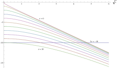
Figure 1:

Bound solutions in two dimensions for $r_{b}=2$. The horizontal line corresponds to $\kappa=-5$.

To find how the number of bound state solutions scale with the boundary radius $r_{b}$, we start by noting that the derivative of the rhs of (11) with respect to $\sqrt{\lambda}$ in the limit $\sqrt{\lambda}\rightarrow 0$ and under the assumption that $n$ is sufficiently greater than $\sqrt{\lambda}$, tends to zero (remark: it turns out that we only need $n>2$ for the argument to work). This implies that the tangent to the curves corresponding to the rhs of (11) are parallel to the $\sqrt{\lambda}$ axis and therefore also to the $\kappa=$ constant curve.

Thus, in the limit $\sqrt{\lambda}\rightarrow 0$ the curve corresponding to some order $n_{m}$ ($>2$, see the remark above) of the modified Bessel function will either be coincident with the $\kappa=\rm{constant}$ curve or will be the first curve not intersecting it at all (in either case the solution corresponding to order $n=n_{m}$ will not be a bound state). Thus, one can find the dependence of the total number of bound state solutions on the radius $r_{b}$ of the removed disc. For this we take the limit $\sqrt{\lambda}\rightarrow 0$ on the rhs of (11) with $n=n_{m}$ and use the approximation

$$K_{\alpha}(x)\approx\frac{\Gamma(\alpha)}{2}\left(\frac{2}{x}\right)^{\alpha}\quad(\sqrt{\alpha+1}\gg x>0)$$ (12)

to obtain

$$\lim_{{\sqrt{\lambda}\rightarrow 0}}{\sqrt{\lambda}}\frac{K_{n_{m}}^{\prime}(\sqrt{\lambda}r_{b})}{K_{n_{m}}(\sqrt{\lambda}r_{b})}=-\frac{n_{m}}{r_{b}}\,.$$ (13)

Equating this to $\kappa$ one finds that $n_{m}$ scales linearly with radius $r_{b}$

$$n_{m}=-\kappa r_{b}\,.$$ (14)

From the arguments presented above, the maximum number of bound state solutions is equal to $n_{m}$ if the rhs of (14) is an integer (the total number of bound state solutions is $n_{m}$ and not $n_{m}-1$ since $n=0$ also corresponds to a bound state solution). If it is not an integer, then the number of bound state solutions is the smallest integer greater than $-\kappa r_{b}$. We also note that except for the case $n=0$ there is a two-fold degeneracy in the number of bound state solutions since $n\rightarrow-n$ gives the same solution.

(a) $E_{n}~{}v/s~{}n$

(b) $<r_{n}>~{}v/s~{}n$

Figure 2:

Energy spectrum $E_{n}$ and the expectation value $<r_{n}>$ in two spatial dimensions for $r_{b}=1$ and $\kappa=-100$.

From (11) it is difficult to obtain an analytic expression for the energy of bound states. However the spectrum can be obtained numerically and in Fig. LABEL:energy_spectrum_2d_solutions and LABEL:expectation_value_of_r_2d_solutions we show the dependence of energy $E_{n}$ and the expectation value $<r_{n}>$ on $n$, the order of bound states, for the choice $\kappa=-100$ and $r_{b}=1$.

From the figure we note that the energy of the lowest state $E_{0}$ is close to $-\kappa^{2}$. The spectrum is approximately given by $E_{n}\approx-\kappa^{2}+n^{2}/r_{b}^{2}$ and thus with increasing $n$ the energy approaches zero. We also note that for all $n$ the expectation value $<r_{n}>$ is always close to $r_{b}$ showing that these states are all localized near the boundary. This is a general feature of the solution as can be verified by choosing different values for $\kappa$ and $r_{b}$.

2.2 3+1 dimensional flat spacetime

We now repeat the above calculations for the case of $\mathbb{R}^{3}-\mathbb{B}^{3}$. Using the expression for the Laplacian in spherical coordinates, the eigenvalue problem to be solved is

$$\frac{1}{r^{2}}\frac{\partial}{\partial r}\left(r^{2}\frac{\partial\psi}{\partial r}\right)+\frac{1}{r^{2}\sin{\theta}}\frac{\partial}{\partial\theta}\left(\sin{\theta}\frac{\partial\psi}{\partial\theta}\right)+\frac{1}{r^{2}\sin^{2}\theta}\frac{\partial^{2}\psi}{\partial\phi^{2}}=\lambda\psi\,,$$ (15)

where as before $\lambda>0$. The above equation can be solved easily by using separation of variables writing $\psi(r,\theta,\phi)=R(r)Y_{lm}(\theta,\phi)$, where $Y_{lm}(\theta,\phi)$’s are the spherical harmonics solving the angular part of the equation. The radial part of the equation is given by (in subsequent analysis we replace $l$ by $n$)

$$\frac{d^{2}R}{dr^{2}}+\frac{2}{r}\frac{dR}{dr}-\frac{n(n+1)R}{r^{2}}=\lambda R\,.$$ (16)

Since the form of the Laplacian is the same as that in (4), it is clear that this again is a self-adjoint operator on the domain of interest. As in the previous case the above equation, with the requirement of square integrability on $(r_{b},\infty)$ with measure $r^{2}dr$, is solved by the modified Bessel function of the second kind $K_{n+\frac{1}{2}}(\sqrt{\lambda}r)$ with the only difference that now the order of the modified Bessel function is $(n+1/2)$. The complete solution to the equation is

$$\psi(r,\theta,\phi)=c\frac{K_{n+\frac{1}{2}}(\sqrt{\lambda}r)}{r^{1/2}}Y_{nm}(\theta,\phi)\,.$$ (17)

We now impose the boundary condition in (2) and as in the two dimensional case we have condition only on the radial solution

$$\kappa R(r_{b})-R^{\prime}(r_{b})=0\,.$$ (18)

After substituting for $R$ this becomes

$$2\kappa=-2\sqrt{\lambda}\frac{K_{n-\frac{1}{2}}(\sqrt{\lambda}r_{b})+K_{n+\frac{3}{2}}(\sqrt{\lambda}r_{b})}{K_{n+\frac{1}{2}}(\sqrt{\lambda}r_{b})}-\frac{1}{r_{b}}\,.$$ (19)

We again find that bound solutions are possible only for $\kappa<0$ and that for a given value of $\kappa$ and $r_{b}$ only a finite number of bound solutions are possible (see Fig. 3).

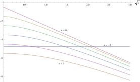
Figure 3:

Bound solutions in three dimensions for $r_{b}=2$. The horizontal line corresponds to $\kappa=-5$.

We find the scaling of the total number of bound state solutions with $r_{b}$ by proceeding exactly as in the two dimensional case. Taking the limit $\sqrt{\lambda}\rightarrow 0$ on the rhs of (19) and using the approximation (12) one finds that

$$\lim_{\sqrt{\lambda}\rightarrow 0}-2\sqrt{\lambda}\frac{K_{n_{m}-\frac{1}{2}}(\sqrt{\lambda}r_{b})+K_{n_{m}+\frac{3}{2}}(\sqrt{\lambda}r_{b})}{K_{n_{m}+\frac{1}{2}}(\sqrt{\lambda}r_{b})}-\frac{1}{r_{b}}=-\frac{(4n_{m}+3)}{r_{b}}\,.$$ (20)

Equating this to $2\kappa$ we find that as in the two dimensional case, $n_{m}$ scales linearly with $r_{b}$ in three dimensions also

$$n_{m}=-\frac{(2\kappa r_{b}+3)}{4}\,.$$ (21)

The number of bound state solutions (ignoring the degeneracy factor) is then given by

$$n_{b} = -\frac{(2\kappa r_{b}+3)}{4}-1\quad\mbox{($n_{m}$ an intger)}\,,$$

$$n_{b} = \lfloor-\frac{(2\kappa r_{b}+3)}{4}\rfloor\quad\quad\mbox{($n_{m}$ not an integer)}\,.$$ (22)

Taking into account the degeneracy in the spherical harmonics, the total number of bound states is given by $\Sigma_{i=0}^{i=b-1}(2n_{i}+1)=n_{b}^{2}$. Using the expression for $n_{b}$ in (2.2) we see that this has terms depending quadratically and linearly on $r_{b}$ as well as a term independent of it. However for $r_{b}\gg 0$, the quadratically dependent term dominates over the other two.

3 The Nonrotating BTZ Black Hole

The analysis of the previous section can be done for black hole spacetimes as well, treating the black hole horizon as a boundary. One of the main interests would be to see whether similar results hold in that case as well. If they do then it would provide a plausible explanation for the origin of black hole entropy without requiring a detailed knowledge of quantum gravity. The picture would be a realization (at least for a large black hole) that the bound states are localized near the horizon and their number (to leading order) is proportional to the area of the black hole.

With these remarks, we now apply the methods of the previous section to the case of BTZ black hole [19]. To simplify calculations we limit ourselves to the case of nonrotating BTZ black holes. We want to obtain the Laplacian for a spatial slice in this background. The main point of the calculation is to do a self-adjointness analysis of the Laplacian and see if it implies mixed boundary condition which, as noted earlier, would introduce a length parameter in the problem that can be taken to be of the order of the Planck length. Thus we will need to identify the Laplacian operator on the BTZ spacetime, the metric for which (in the nonrotating case) is given by

$$ds^{2}=g_{\alpha\beta}dx^{\alpha}dx^{\beta}=-\frac{(r^{2}-r_{+}^{2})}{l^{2}}dt^{2}+\frac{l^{2}}{(r^{2}-r_{+}^{2})}dr^{2}+r^{2}d\theta^{2}\,,$$ (23)

where $r_{+}$ corresponds to the horizon and $l^{2}$ is the negative inverse of the cosmological constant. The massive Klein-Gordon equation is given by

$$(\square-m^{2})\phi=\frac{1}{\sqrt{-g}}\partial_{\alpha}(\sqrt{-g}g^{\alpha\beta}\partial_{\beta})\phi-m^{2}\phi=0\,,$$ (24)

where $g^{\alpha\beta}$ is the inverse of the metric in (23) and $\sqrt{-g}$ is its determinant. Using (23) in (24) we get

$$-\frac{l^{2}}{(r^{2}-r_{+}^{2})}\partial_{t}^{2}\phi+\frac{1}{r}\partial_{r}\left[\frac{r(r^{2}-r_{+}^{2})}{l^{2}}\partial_{r}\right]\phi+\frac{1}{r^{2}}\partial_{\theta}^{2}\phi-m^{2}\phi=0\,.$$ (25)

This equation has been analyzed in detail at several places, see [20] for instance, and it is known that the equation can be solved exactly.

3.1 The measure in the $r$ coordinate

We are interested in the self-adjointness of the Laplacian which requires a suitable measure (defining the inner product) on the Hilbert space. In a general curved background the scalar product is defined by [21]

$$(\phi_{1},\phi_{2})=-i\int_{\Sigma}[\phi_{1}(\partial_{\mu}\phi_{2}^{*})-(\partial_{\mu}\phi_{1})\phi_{2}^{*}]\sqrt{g_{{}_{\Sigma}}}n^{\mu}d\Sigma\,.$$ (26)

Here $n^{\mu}$ is the future directed unit vector orthogonal to spacelike hypersurface $\Sigma$; $g_{{}_{\Sigma}}$ is the determinant of the metric on the hypersurface with $d\Sigma=drd\theta$ being the volume element on it. For the BTZ metric, (23), the unit normal to the hypersurface is given by $g^{\alpha\beta}n_{\alpha}n_{\beta}=g^{tt}n_{t}n_{t}=-1$. This implies that the only nonzero component of $n^{\mu}$ is $n^{t}=-l/(r^{2}-r_{+}^{2})^{1/2}$. We also have $\sqrt{g_{{}_{\Sigma}}}=lr/(r^{2}-r_{+}^{2})^{1/2}$ and $d\Sigma=drd\theta$. Thus the inner product for nonrotating BTZ is given by

$$(\phi_{1},\phi_{2})=i\int_{\Sigma}[\phi_{1}(\partial_{t}\phi_{2}^{*})-(\partial_{t}\phi_{1})\phi_{2}^{*}]\frac{l^{2}r}{(r^{2}-r_{+}^{2})}drd\theta\,.$$ (27)

Note that the measure diverges near the horizon (this is related to the redshift).

3.2 Equations in tortoise coordinates

It turns out that the problem can be translated in the form of standard Schroedinger equation by going to the tortoise coordinates. This also makes the analysis of self-adjointness issue easier. We use the ansatz $\phi=e^{-i\omega t}e^{in\theta}\frac{f(r)}{\sqrt{r}}$ in Eq. (25) and obtain

$$\frac{(r^{2}-r_{+}^{2})}{l^{2}}\frac{d^{2}f}{dr^{2}}+\frac{2r}{l^{2}}\frac{df}{dr}-\frac{3f}{4l^{2}}-\frac{r_{+}^{2}f}{4r^{2}l^{2}}+\frac{l^{2}\omega^{2}f}{r^{2}-r_{+}^{2}}-\frac{n^{2}f}{r^{2}}-m^{2}f=0\,.$$ (28)

To aid further calculations we now go to the tortoise coordinates which are effected by the transformation

$$dr_{*} = \frac{l^{2}}{r^{2}-r_{+}^{2}}dr,$$

$$r_{*} = -\frac{l^{2}}{r_{+}}\coth^{-1}\left(\frac{r}{r_{+}}\right),$$

$$r = -r_{+}\coth\left(\frac{r_{+}r_{*}}{l^{2}}\right)\,.$$ (29)

Note that the horizon $r=r_{+}$ in tortoise coordinates is at $r_{*}=-\infty$ and spatial infinity is at $r_{*}=0$. Computing $\partial_{r}f$ and $\partial_{r}^{2}f$ and substituting in (28) we get

$$\frac{d^{2}f}{dr_{*}^{2}}-\left(\frac{3r^{2}}{4l^{4}}-\frac{M}{2l^{2}}-\frac{M^{2}}{4r^{2}}+\frac{n^{2}}{l^{2}}-\frac{Mn^{2}}{r^{2}}+\frac{m^{2}r^{2}}{l^{2}}-m^{2}M\right)f+\omega^{2}f=0\,.$$ (30)

We now transform Eq. (30) entirely in terms of $r_{*}$

$$-\frac{d^{2}f}{dr_{*}^{2}}+\frac{1}{\sinh^{2}(\alpha r_{*})}\left(\frac{3\alpha^{2}}{4}+m^{2}M\right)f+\frac{1}{\cosh^{2}(\alpha r_{*})}\left(\frac{\alpha^{2}}{4}+\frac{n^{2}}{l^{2}}\right)f=\omega^{2}f\,,$$ (31)

where we have used the notation $\alpha=\sqrt{M}/l$ (we also note that the horizon is given by $r_{+}=l\sqrt{M}$, $M$ being the mass of the black hole). This equation is in the form of standard Schroedinger equation

$$-\frac{d^{2}\psi(r_{*})}{dr_{*}^{2}}+V(r_{*})\psi(r_{*})=\omega^{2}\psi(r_{*})$$

with the potential

$$V=\frac{1}{\sinh^{2}(\alpha r_{*})}\left(\frac{3\alpha^{2}}{4}+m^{2}M\right)+\frac{1}{\cosh^{2}(\alpha r_{*})}\left(\frac{\alpha^{2}}{4}+\frac{n^{2}}{l^{2}}\right)\,.$$ (32)

We now need to write the scalar product in terms of the $r_{*}$ coordinate and for this we note that in the ansatz $\phi=e^{-i\omega t}e^{in\theta}\frac{f(r)}{\sqrt{r}}$ there is an explicit factor of $\sqrt{r}$ sitting in the denominator. The two factors of $\phi$ in the scalar product will thus contribute a factor of $r^{-1}$ which will cancel the $r$ in the numerator of (27). Thus, in terms of the tortoise coordinates the integration measure is simply $dr_{*}$. It is now straight forward to verify that the Laplacian is a self-adjoint operator for the boundary condition $\kappa f=df/dr_{*}$ imposed at the horizon $r_{*}=-\infty$. This is of the same form as the condition we had in the previous section on flat backgrounds.

Knowing the appropriate boundary condition that makes the Hamiltonian operator self-adjoint, we can now go back to the $r$ coordinate in terms of which the boundary condition is

$$Ag(r)+(r-r_{+})\partial_{r}g(r)=0\,,$$ (33)

where $g(r)$ is the solution of the radial part of the Laplacian in the original coordinates. In the above equation both sides are evaluated at $r=r_{+}$ and $A$ is a constant depending on $\kappa,r_{+},l$.

Having obtained the conditions for self-adjointness in (33) the analysis requires numerical computations. This is not completed because of strong oscillations of solutions near the horizon for generic boundary values. But we will argue that analysis will lead to similar results.

Equation (30) is the Hamiltonian eigenvalue equation in 1-dimension for each value of n. Comparing this with similar Eq. (4) we find that the self-adjointness condition can be satisfied only for finite $n$ up to some maximum value $n_{m}$. The eigenvalues are negative and $\propto-\kappa^{2}$ since contributions come from the second order derivative term in (28) satisfying boundary conditions. These are close to the boundary. From our flat space computations it is clear that the number of bound states is finite and proportional to $r_{+}$ $(r_{+}^{2})$ in two dimensions (three dimensions). The same result continues to be true even in the BTZ case as can be seen by near horizon analysis of solutions of (28) satisfying the boundary conditions (33), though obtaining the exact number of solutions looks difficult. The reason for this is that in the Hamiltonian (30), we see that for large $r$ there is a term in the potential which is proportional to $r^{2}$ like the harmonic oscillator. Hence, the spectrum has eigenvalues which are positive and wave functions are supported over a larger length scale controlled by cosmological constant. We should separate the two kinds of states, and this can be analyzed in the large $r_{+}\gg l\gg 1/\kappa$ regime. This problem is akin to self-adjointness for harmonic oscillator on $\mathbb{R}^{2}-\mathbb{D}$. Furthermore the boundary (horizon), which is at $r_{*}=-\infty$, is actually located at a finite distance $r_{+}$ in usual coordinates. Hence the self-adjointness condition is related to the dilatation operator $(r-r_{+})\partial_{r}$ near the horizon. The scaling operator along with the Hamiltonian forms elements of an SL(2,R) algebra which has been used through conformal quantum mechanics to understand the near horizon dynamics [22, 23].

4 Discussion

In this paper we find novel bound state solutions for Laplacian on manifolds with boundary. These arise by requiring it to be self-adjoint. These states are localized close to the boundary and serve to explain the states of a black hole contributing to the entropy. They also contribute to Hawking radiation which will be explored later. These features arise through brickwall mechanism and quantum mechanical origin justifying the boundary conditions on the horizon. The horizon states can be compared with membrane paradigm also [24, 25]. They can also be looked as states obtained from spin network of LQG though our states contribute directly to energy whereas spin network give area bits.

In this connection we wish to point out an interesting result from [14]. Here a general analysis is done for self-adjoint extensions and the most general boundary conditions are characterized by an infinite dimensional unitary matrix linking the boundary data. It is given by

$$(\phi+i\partial_{\overrightarrow{n}}\phi)=U(\phi-i\partial_{\overrightarrow{n}}\phi)$$ (34)

evaluated at the boundary and $\overrightarrow{n}$ stands for the normal. They also point out that if $U$ has an eigenvalue $-1$ then the extensions given by $Ue^{-it}$ have a negative energy state which is an edge state. They are characterized by the length parameter. However, when the Hamiltonian has in addition potential term which contributes positive energy to the state which increases with $n$, then there is a balance of these contributions resulting in finite number of states. This results in the number of edge states being constrained by the radius.

In the case of Schwarzschild black hole the situation is different since it is asymptotically flat. This work is in progress and will be presented elsewhere.

References

- [1] J.D. Bekenstein, Phys. Rev. D 7, 2333 (1973).
- [2] S.W. Hawking, Comm. Math. Phys. 43, 199 (1975).
- [3] A. Strominger and C. Vafa, Phys. Lett. B 379, 99 (1996).
- [4] A. Ashtekar, J. Baez, A. Corichi and K. Krasnov, Phys. Rev. Lett. 80, 904 (1998).
- [5] R.K. Kaul and P. Majumdar, Phys. Rev. Lett. 84, 5255 (2000).
- [6] S. Carlip, Phys. Rev. Lett. 82, 2828 (1999).
- [7] T. Padmanabhan, Rept. Prog. Phys. 73, 046901 (2010).
- [8] L.Bombelli, R.K. Koul, J. Lee and R.D. Sorkin, Phys. Rev. D 34, 373 (1986); M. Srednicki, Phys. Rev. Lett. 71, 666 (1993); S. Das, S. Shankaranarayanan and S. Sur, arXiv:0806.0402.
- [9] G. ’t Hooft, Nucl. Phys. B 256, 727 (1985).
- [10] G. ’t Hooft, Int. Jour. Mod. Phys. A11, 4623 (1996).
- [11] J.D. Bekenstein, Lett. Nuovo Cim. 11, 467 (1974).
- [12] J.D. Bekenstein and V.F. Mukhanov, Phys. Lett. B 360, 7 (1995).
- [13] T.R. Govindarajan, V. Suneeta and S. Vaidya, Nucl. Phys. B 583, 291 (2000).
- [14] M. Asorey, A. Ibort and G. Marmo, Int. Jour. Mod. Phys. A20, 1001 (2005).
- [15] S.K. Chakrabarti, P.R. Giri and K.S. Gupta, Eur. Phys. Jour. C60, 169 (2009).
- [16] M.V. Berry amd M.R. Dennis, Jour. Phys. A: Math. Theo. 41, 135203 (2008).
- [17] M. Reed and B. Simon, Methods of Modern Mathematical Physics Vol. I-IV (Academic Press) (1980).
- [18] Kumar S. Gupta (private communication).
- [19] M. Banados, C. Teitelboim and J. Zanelli, Phys. Rev. Lett. 69, 1849 (1992).
- [20] I. Ichinose and Y. Satoh, Nucl. Phys. B 447, 340 (1995).
- [21] N.D. Birrell and P.C.W. Davies, Quantum Fields in curved space (Cambridge University Press, Cambridge) (1984).
- [22] H.E. Camblong and C.R. Ordonez, Phys. Rev. D 71, 104029 (2005).
- [23] D. Birmingham, Kumar S. Gupta and S. Sen, Phys. Lett. B 505, 191 (2001).
- [24] T. Damour, Phys. Rev. D 18, 3598 (1978).
- [25] R.H. Price and K.S. Thorne, Phys. Rev. D 33, 915 (1986).