Determination of the zeta potential for highly charged colloidal suspensions

Abstract

Zeta-potential, electrophoresis, lattice-Boltzmann, mesoscopic models, electrostatic radius. We compute the electrostatic potential at the surface, or zeta potential $\zeta$, of a charged particle embedded in a colloidal suspension using a hybrid mesoscopic model. We show that for weakly perturbing electric fields, the value of $\zeta$ obtained at steady state during electrophoresis is statistically indistinguishable from $\zeta$ in thermodynamic equilibrium. We quantify the effect of counterions concentration on $\zeta$. We also evaluate the relevance of the lattice resolution for the calculation of $\zeta$ and discuss how to identify the effective electrostatic radius.

1 Introduction

A quantitative understanding of the electrostatic interactions between charged macroions in solution is fundamental to comprehend a plethora of physical phenomena spanning from biology to material science, for example the macroscopic and rheological properties of colloidal suspensions[1,2]. The details of such interactions are difficult to capture, as the effective interactions are determined by the interplay between the different components dissolved in solution (macroions, counterions, salt ions) and the solvent dielectric response[3]. In addition, when the system is driven out of equilibrium, for example by an external electric field causing electrophoretic flow, hydrodynamic interactions between the solvent and solute species must also be included and can alter the equilibrium electrostatic interactions.

The simplest yet very useful model to describe electrolyte solutions is the Poisson-Boltzmann (PB) approach[1,4], which builds on a continuous description of the electrolyte, characterized in terms of the anion and cation local densities. Within this framework, it is possible to add charged macroscopic objects, with fixed surface charges, by accordingly changing the electrostatic boundary conditions of the PB equations. Notwithstanding PB is a mean-field theory that defines ions as point-like and therefore neglects excluded volume effects and spatial correlation due to their finite size, it has been successfully adopted to describe various physical systems, for example to derive the electrostatic part of DLVO interparticle potential[1] which explains the interactions of weakly charged particles in solution at low volume fraction.

The zeta potential, $\zeta$, defined as the electrostatic potential at the colloid surface, or slippling plane, plays a central role for charged colloidal dispersions, as it indirectly provides an estimate of the magnitude of the electric field between particles that results from the combined effect of ionized charged groups sitting on the particle, counterions released into solution and salt ions. Theoretically, Ohshima et al.[5] obtained an exact analytic expression relating the surface charge density to the zeta potential for an infinitely dilute spherical colloidal suspension by carefully approximating the non-linear PB equation. This expression is of limited use, since the infinite dilution regime is difficult to achieve. Moreover, experimentally $\zeta$ is normally derived out of equilibrium, from electrophoretic mobility measurements. Since, a priori, the values of $\zeta$ in equilibrium and at steady state will differ, an accurate description of hydrodynamics must be included in order to derive the relationship between $\zeta$ and the colloid mobility.

Analytical results for the electrophoretic flow at finite dilution cannot in general be obtained. Computationally, different models have been used to describe electrophoresis[6-9,11]. Lobaskin et al.[8] and Dünweg et al[9], using a lattice Boltzmann[10] (LB) solver coupled to molecular dynamics of ions, calculate the particle mobility for low to zero salt concentration explicitly accounting for finite ions size, but without providing results for $\zeta$. Kim et al.[11] show agreement with Ohshima’s results, but only for weakly charged particles at low salt concentration. Cell models[12] are also employed to describe electrokinetics and to derive mobility versus $\zeta$ curves; however, they rely on somewhat arbitrary boundary conditions both for electrostatics and hydrodynamics.

In this paper, we compute $\zeta$ using a mesoscopic model that couples a Navier-Stokes solver to the convection and diffusion of ions on a lattice. We will first investigate the difference between $\zeta$ values at thermodynamic equilibrium and at electrophoretic steady state. We then accurately analyze the dependence of $\zeta$ on colloid volume fraction, $\Phi$, and salt and counterions concentration, and compare them with predictions from PB at infinite dilution derived by Ohshima et al.[5]. Finally, we will address how to identify the electrostatic radius of a colloid on a lattice, as it has been done previously for the hydrodynamics radius[13]. In the following section, we briefly introduce our model, the reference equations and results that can be obtained using PB equation for infinite dilution and at finite volume fractions. We present in section 3 results for $\zeta$ as a function of the volume fraction, salt concentration and lattice refinement. Finally, we draw our main conclusions in the last section.

2 Model

2.1 Electrophoretic flow

In order to derive a correct relation between the mobility and the zeta potential at steady state during electrophoresis, our model includes hydrodynamic interactions and electric forces due to local charge densities,

$$\frac{\partial\rho_{k}}{\partial t}=-\nabla\cdot\rho_{k}\vec{v}+\nabla\cdot D_{k}[\nabla\rho_{k}+e\beta z_{k}\rho_{k}\nabla\varphi],$$ (1)

$$\frac{\partial(\rho\vec{v})}{\partial t}=\eta\nabla^{2}\vec{v}-\nabla p_{id}+\beta\sum_{k}ez_{k}\rho_{k}\nabla\varphi,$$ (2)

$$\nabla^{2}\varphi=-\frac{1}{\epsilon}\sum_{k}ez_{k}\rho_{k},$$ (3)

where $D_{k},z_{k},k=+,-$ are the diffusivities and valences of positive and negative ions, $\rho,\vec{v},p_{id}$ and $\eta$ correspond to the solvent density, velocity, ideal pressure and shear viscosity, $e$ is the electron charge, $\beta^{-1}=k_{B}T$ is the Boltzmann factor, $\varphi$ is the electrostatic potential and $\epsilon$ the solvent permittivity. Eq. 1 expresses ions mass conservation during diffusion and advection, coupling ion dynamics to solvent motion. This is in turn described by the Navier-Stokes equation for a viscous fluid which couples solvent dynamics to electrostatic forces due to local charge density, Eq. 2. Finally, the Poisson equation enforces the electrostatic coupling between the charged species and the embedded solid particles. We solve these electrokinetics equations combining an LB approach for the momentum dynamics with a numerical solver for the discretized convection-diffusion dynamics, Eq. (1), based on link fluxes[14]. Each lattice site is labeled as solid or fluid and we consider here a single spherical object of radius $r=a$ embedded in a cubic lattice of volume $L^{3}$ with periodic boundary conditions. Suspended particles are therefore resolved and interact with the neighbouring fluid through bounce-back[13]. The electrostatic potential is computed using a successive over-relaxation scheme (SOR)[16]. This method has been successfully applied to analyze different dynamical processes involving suspensions of charged objects[15,17,18,19].

2.2 Poisson-Boltzmann electrostatics

At equilibrium, using a mean-field approach that neglects excluded volume effects and correlation between ions, PB equation reads[4]

$$\nabla^{2}\varphi(\vec{r})=\frac{8\pi ez\rho_{0}}{\epsilon}\sinh(\frac{ez\varphi(\vec{r})}{k_{B}T}),$$ (4)

where a symmetric electrolyte $z_{+}=z_{-}=z$ has been used for simplicity and $\rho_{0}$, the uniform macroscopic counterion and coion number concentration far from the colloid $\rho_{+}=\rho_{-}=\rho_{0}$, is assumed to be equal to that of an electrolyte reservoir with dissolved salt $c_{salt}=2\rho_{0}$.

An analytical solution of eq. (4) for a single particle is not available, as the PB equation can be solved analytically only for a few symmetrical configurations. Ohshima et al.[5] analyzed eq. (4) around a spherical colloid of charge $Q$ using a perturbative approach and derived a quasi-exact analytical expression for $\zeta$,

$$Q=2\frac{ea^{2}}{\lambda_{D}l_{B}}\sinh(\tilde{\zeta}/2)\left[1+\frac{2}{(\kappa a)\cosh^{2}(\tilde{\zeta}/4)}+\frac{8\log(\cosh^{2}(\tilde{\zeta}/4))}{(\kappa a)^{2}\sinh^{2}(\tilde{\zeta}/2)}\right]^{1/2},$$ (5)

where $\kappa=\sqrt{\frac{4\pi e^{2}z^{2}c_{salt}}{\epsilon k_{B}T}}=\lambda_{D}^{-1}$ is the inverse of the Debye length, $l_{b}=\frac{e^{2}}{4\pi\epsilon k_{B}T}$ the Bjerrun length and $\tilde{\zeta}=\frac{e\zeta}{k_{B}T}$ the adimensional zeta potential.

Useful global information can be obtained using the Debye-Hückel approximation, i.e. linearizing eq. (4). When $\frac{ez\varphi}{k_{B}T}\lesssim 1.0$,

$$\nabla^{2}\varphi(\vec{r})=\frac{4\pi e^{2}z^{2}\rho_{0}}{\epsilon k_{B}T}\varphi(\vec{r})=\kappa^{2}\varphi(\vec{r}).$$ (6)

from which one can derive the electrostatic potential around a charged spherical colloid

$$\varphi(r)=\frac{\zeta a}{r}\exp^{(-(r-a)/\lambda_{D})}.$$ (7)

In the linear regime, a charged particle in the presence of salt develops a screened, Yukawa-like electrostatic potential, with a characteristic length scale of $\lambda_{D}$ and strength given by the zeta potential, $\zeta$.

Eq.(4) is strictly valid when the amounts of positive and negative charges dissolved in solution are equal, i.e. when the counterions concentration is negligible. Experimentally, this can be obtained separating the colloidal particles from a bulk electrolyte solution with a semi-permeable membrane. For the experimental set-ups with non-zero concentration of counterions, eq. (6) becomes

$$\nabla^{2}\varphi(r)=\kappa^{2}\left[\frac{\rho_{c0}}{2\rho_{s0}}+(1+\frac{\rho_{c0}}{2\rho_{s0}})\varphi(r)\right],$$ (8)

where $\rho_{s0},\rho_{c0}$ are the reference salt and counterion concentrations in the reservoir. Eq. (8) stresses the fact that, especially at low salt concentration $c_{s}$ (low $\rho_{s0}$) and high volume fraction $\phi=\frac{4\pi a^{3}}{L^{3}}$ (high $\rho_{c0}$), a deviation from the theoretical Debye-Hückel results can be observed.

Our aim is to measure $\zeta$ for different experimental regimes, analyze its behavior beyond the linear approximation (when $\frac{e\varphi}{k_{B}T}\gtrsim 1$) and understand how to overcome the intrinsic inaccuracies in the location of the electrostatic radius of any lattice model. In the LB approach, we will refer to $\zeta$ as the average electrostatic potential between lattice points pairs (boundary links) $l$ that link a colloid and a fluid node calculated half-way between the two nodes using linear approximation,

$$\zeta_{MP}=\left<\sum_{l}\frac{\varphi_{solid}(l)+\varphi_{fluid}(l)}{2}\right>.$$ (9)

and will analyze when such an assumption is representative of the colloid $\zeta$.

3 Results

We have performed simulations for a single spherical particle of radius $a$ embedded in cubic boxes with periodic boundary conditions, also varying the concentration of added salt. In order to avoid finite-size effects, for a given salt concentration we use a lattice length L at least three times the corresponding Debye length, $\lambda_{D}$. We have distributed uniformly the colloid charge $Q$ on the lattice sites the colloid fills, and choose $Q$ to correspond to the predicted value of Oshima, according to eq.(5). We will analyze both a magnitude of $Q$ which lies in the linear regime, $\tilde{\zeta}_{O}=1.0$, and one for which the colloid is within the nonlinear regime, $\tilde{\zeta}_{O}=5.0$. We finally set the external electric field to $E=0.01$, well within the linear regime $E\ll\frac{\zeta}{\lambda_{D}}$.

The values for $\zeta$ obtained from electrophoresis are in principle different from those computed in equilibrium. This is analogous to the different measurements for the size of a solvated particle, at equilibrium or at hydrodynamic steady state (hydrodynamic radius). We have therefore computed $\tilde{\zeta}_{MP}$ at thermodynamic equilibrium, i.e. with equilibrated charges and fluid at rest and dynamically, when a steady state due to the external electric field is reached. In all simulations, our results show that the differences between the two values of $\zeta$ are smaller than the statistical precision. This similarity is expected because of the small magnitude of the perturbing electric field and colloid Péclet number, $Pe=\frac{av_{coll}}{D_{\pm}}$, where $v_{coll}$ is the velocity of the colloid at steady state. For $Pe\geq 1$ the deformation of the salt cloud around the colloid induces significant deviations in the electrophoretic mobility[18]; we can hence envisage a corresponding departure of the dynamic $\zeta$ from its equilibrium counterpart. Typically, as for simulations here, $Pe\ll 1$ and particle mobility does not depend on $Pe$, hence the measured $\zeta$ values at equilibrium and steady state are statistically indistinguishable.

As the only theoretical result available, $\tilde{\zeta}_{O}$, is valid for a single particle in equilibrium at infinite dilution, we will compare the simulation results with eq.(5) to assess the role of the counterion concentration at finite volume fraction. In addition, in order to analyze to which extent the midpoint stands as a proper definition for the electrostatic radius, we run a pair of simulations for each colloid charge, volume fraction and salt concentration used, changing the resolution of the colloid in the lattice from low, using colloid radius $a=4.5$, to high $a=9.0$, also doubling the corresponding box sizes (e.g. from $L=30$ at low resolution to $L=60$ at high resolution for the highest volume fraction).

 

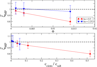
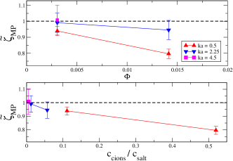
Figure 1: Left(Right): Electrostatic potential $\tilde{\zeta}_{MP}$ calculated halfway between boundary links (see text for definition) using a low(high)-resolution lattice. Colloidal charges for different salt concentrations ($ka=0.5,2.25,4.5$) have been assigned so that the resulting theoretical zeta potential (eq. (5)) is within the linear electrostatic, Debye-Hückel regime ($\tilde{\zeta}_{O}=1.0$, dashed line)

Fig.1 displays $\tilde{\zeta}_{MP}$ for a weakly charged colloid ($\tilde{\zeta}_{O}=1.0$) as a function of the system size and salt concentrations, where the left(right) panel corresponds to a low(high) colloid resolution. The top panels show that the deviation of $\tilde{\zeta}$ from Oshima’s prediction varying $\Phi$ appears indirectly only through the corresponding change in the co- and counter-ion concentrations because the deviation decreases when the salt concentration is increased. Therefore, according to eq. (8), we can gain understanding by analyzing the dependence of $\tilde{\zeta}_{MP}$ on the ratio between the concentration of counterions released by the particle, $c_{cions}$ (which decreases as $\Phi$ increases ) and the concentration of salt $c_{salt}$ dissolved in the system (which is independent of $\Phi$). The bottom panels confirm an agreement within $10\%$ between $\tilde{\zeta}_{MP}$ and $\tilde{\zeta}_{O}$ for $\frac{c_{cions}}{{c_{salt}}}\lesssim 0.1$. In addition, comparing the left and right panels, we conclude that in the linear regime the lattice resolution does not play a significant role, as for a given salt concentration $\tilde{\zeta}_{MP}$ does not differ significantly and the use of a more computationally expensive refined lattice only reduces the error bars. In addition, we note from bottom-rigth panel that discretization effects become more relevant when increasing the salt concentration. This sensitivity is associated to the reduction of $\lambda_{D}$ and the corresponding loss of resolution in the electrostatic potential around the colloid.

Fig. 2, organized analogously to Fig. 1, shows results for a strongly charged colloid, $\tilde{\zeta}_{O}=5.0$, for which the linearized Debye-Hückel approximation does not hold. We observe that the dependence of $\tilde{\zeta}_{MP}$ on $\Phi$ enters again indirectly through the relative changes in $c_{cions}$, and that the convergence toward $\tilde{\zeta}_{O}$ can only be expected for high $c_{salt}$. However, as opposed to the linearized regime, adding salt can lead up to a $20\%$ overestimation of $\tilde{\zeta}_{MP}$ for the highest salt concentration analyzed ($ka=4.5$), especially when using a low resolution lattice (left panels). In this strong coupling regime the electrostatic potential decays faster than $\lambda_{D}$[1]. This strong nonlinear behavior invalidates the midpoint as the natural choice for the electrostatic radius, which develops a dependence on the system parameters even when the effects of finite $\Phi$ and $c_{cions}$ are negligible.

 

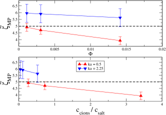
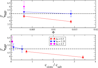
Figure 2: Left(Right): Electrostatic potential $\tilde{\zeta}_{MP}$ calculated halfway between boundary links (see text for definition) using a low(high)-resolution lattice. Colloidal charges for different salt concentrations ($ka=0.5,2.25,4.5$) have been assigned to obtain a theoretical zeta potential (eq. (5), dashed line) $\tilde{\zeta}_{O}=5.0$, within the nonlinear regime

Fig. 3 displays the measured electrostatic potential at the midpoint between a solid and fluid node, $\tilde{\zeta}_{MP}$, together with the two extreme situations where the electrostatic potential is averaged over the solid and the fluid nodes corresponding to the boundary links. One can observe, as expected, that $\tilde{\zeta}_{MP}$ always lies in between the other two estimates of $\tilde{\zeta}$. The differences observed between the left and right panels indicate that the increase in resolution does not affect significantly $\tilde{\zeta}_{MP}$, while decreases the inaccuracy in the estimate of the limiting values for $\tilde{\zeta}$. Generically, the better resolved the colloidal particle (and the corresponding decay of the electrostatic potential, $\varphi$) the less spreading between the different electrostatic potential estimates. When we increase $c_{cions}$, Oshima’s prediction does no longer hold and eq. (5) cannot be used to identify the electrostatic radius as can be appreciated in the rightmost values of $\tilde{\zeta}$ in the bottom panels. However, the weak dependence of $\varphi$ in the boundary fluid nodes suggests that when $\tilde{\zeta}_{MP}$ is no longer valid, we can still identify a electrostatic radius slightly larger than the one associated to $\tilde{\zeta}_{MP}$. Analogously to the hydrodynamic radius, an ad hoc calibration of the electrostatic radius at all salt concentrations must be done to perform quantitative studies of the electrokinetics of colloidal suspensions with LB.

 

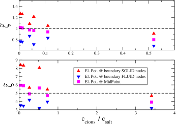
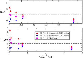
Figure 3: Left[Right]: Average electrostatic potential calculated using low[high] resolution lattice at midpoint (squares), solid (triangle-up) and fluid (triangle-down) nodes pertaining to boundary links in all simulation set-ups ($ka=0.5,2.25,4.5$, $\tilde{\zeta}_{O}=1.0,5.0$). Top[Bottom] panels correspond to the case of a weakly [strongly] charged colloid.

4 Conclusions

In this paper, we have analyzed how to determine the electrostatic potential at the surface of a particle, or zeta potential $\zeta$, for a colloidal suspension. To this end, we have made use of a hybrid mesoscopic model which couples a discrete lattice formulation of Boltzmann’s kinetic equation for the solvent to a discrete solution of the convection-diffusion equation for the charged ion species dissolved in the fluid which implies treating counter- and salt ions as scalar fields at the Poisson-Boltzmann (PB) level. We have found that for weakly perturbing electric fields, it is not possible to distinguish between the equilibrium and dynamic zeta potentials. We expect differences will arise when the deformation of the charge layer around the colloid becomes significant, a scenario which can be achieved, e.g. when the Péclet number of the dissolved ions is not negligible.

In particular, the comparison with Oshima’s expression for $\tilde{\zeta}$ at infinite dilution has allowed us to carry out quantitative checks to validate the code performance. We have seen that the counterion concentration has a significant effect on $\tilde{\zeta}$, leading to a decrease in its magnitude both in the linear and nonlinear regimes away from Oshima’s result. We have shown that the ratio between counterion and salt concentration controls the departure from Oshima’s prediction, and that its prediction works reasonably well for $c_{cions}/c_{salt}\lesssim 0.1$. We have also assessed the relevance of the lattice resolution and have quantified its effects. We have seen that the mean of $\tilde{\zeta}$ over the boundary nodes which determine the colloidal shape is in general a good estimate of the electrostatic radius. However, for highly charged colloids a more refined choice of the particle radius will be in general needed. The effective radius will be slightly larger than predicted from $\tilde{\zeta}_{MP}$ due to the nonlinear decay of the electrostatic potential around the particle. This effective electrostatic radius, which needs to be calibrated as a function of the salt concentration and particle radius, will in general differ from the particle hydrodynamic radius and requires a separate analysis. The overall dependence of the electrostatic radius both on the applied field and ion concentrations is weaker than the one observed for the hydrodynamic radius. In most situations we expect that an equilibrium calibration correcting from the finite counterion concentration will provide a quantitative estimate for the electrokinetics of colloidal suspensions.

5 Acknowledgements

G.G. acknowledges support from the IEF Marie Curie scheme. I.P. acknowledges financial support from Dirección General de Investigación (Spain) and DURSI under projects FIS 2008-04386 and 2009SGR-634, respectively.

References

- (1) [1] W. B. Russel, D. A. Saville, W. R. Schowalter;Colloidal dispersions, Cambridge University Press ,1991
- (2) [2] R. G. Larson;The structure and rheology of complex fluids, Oxford University Press ,1999
- (3) [3] B. Rotenberg, I. Pagonabarraga, D. Frenkel; Faraday Disc., 144, 223 (2010)
- (4) [4] J. L. Barrat, J. P. Hansen;Basic concepts for simple and complex liquids, Cambridge University Press ,2003
- (5) [5] H. Ohshima, T. W. Healy, L. R. White; J. Colloid Interface Sci., 90 , 17–26 (1982)
- (6) [6] A. Chatterji, J. Horbach; J. Chem. Phys. 126, 064907 (2006)
- (7) [7] S. Melchionna, S. Succi; J. Chem. Phys. 120, 4492–4497 (2003)
- (8) [8] V. Lobaskin, B. Dünweg, M. Medebach, T. Palberg, C. Holm; Phys. Rev. Lett., 98 , 176105 (2007)
- (9) [9] B. Dünweg, V. Lobaskin, K. Seethalakshmy-Hariharan, C. Holm; J. Phys.: Condensed Matter , 20, 404214 (2008)
- (10) [10] R. Benzi, S. Succi, M. Vergassola; Phys. Rep. , 222, 145-197 (1992)
- (11) [11] K. Kim, Y. Nakayama, R. Yamamoto; Phys. Rev. Lett., 96, 208302 (2008)
- (12) [12] F. Carrique, J. Cuquejo, F. J. Arroyo, A. V. Jiménez, M. L. , Delgado; Adv. Colloid Interface Sci., 118 , 43–50 (2005)
- (13) [13] A. J. C. Ladd; J. Fluid Mech., 271, 285 (1994); íbid. 271, 310 (1994)
- (14) [14] I. Pagonabarraga, B. Rotenberg, D. Frenkel; Phys. Chem. Chem. Phys. 12, 9566 (2010)
- (15) [15] F. Capuani, I. Pagonabarraga, D. Frenkel; J. Chem. Phys., 121, 973 (2004)
- (16) [16] W. H. Press; Numerical recipes: the art of scientific computing, Cambridge University Press, 2007
- (17) [17] F. Capuani, I. Pagonabarraga, D. Frenkel; J. Chem. Phys., 124, 124903 (2006)
- (18) [18] G. Giupponi, I. Pagonabarraga; Submitted
- (19) [19] B. Rotenberg, I. Pagonabarraga, D. Frenkel; EPL 83, 34004 (2008)