Robustness of networks against propagating attacks under vaccination strategies

Abstract

We study the effect of vaccination on robustness of networks against propagating attacks that obey the susceptible-infected-removed model. By extending the generating function formalism developed by Newman (2005), we analytically determine the robustness of networks that depends on the vaccination parameters. We consider the random defense where nodes are vaccinated randomly and the degree-based defense where hubs are preferentially vaccinated. We show that when vaccines are inefficient, the random graph is more robust against propagating attacks than the scale-free network. When vaccines are relatively efficient, the scale-free network with the degree-based defense is more robust than the random graph with the random defense and the scale-free network with the random defense.

1 Introduction

Many real networks, such as the WWW, the Internet, social and biological networks, have complex connectivity. A property shared by many types of networks is the scale-free (SF) degree distribution $p_{k}\propto k^{-\gamma}$, where $k$ is degree (number of links connected to a node) and $p_{k}$ is the fraction of nodes with degree $k$ [1]. Functions of networks crucially depend on the degree distribution and other structural properties of networks [2, 3, 4, 5, 6, 7, 8].

An important property of networks is robustness against the removal of nodes caused by failures or intentional attacks. Albert et al. studied the robustness of networks against two types of attacks: random failure, where nodes are sequentially removed with equal probability, and intentional attack, where hubs (i.e., nodes with large degrees) are preferentially removed [9]. They showed that SF networks having $\gamma\leq 3$ are highly robust against the random failure in the sense that almost all nodes have to be removed to disintegrate a SF network. However, SF networks are fragile to the intentional attack in the sense that the network is destroyed if a small fraction of hubs are removed. These results have been analytically established [10, 11, 12]. The robustness of networks against other percolation-like processes such as the betweenness-based attack [13] and degree-weighted attacks [14] have also been studied.

In fact, attacks to networks may occur as propagating processes. Examples include computer viruses [15, 16, 17]. The (first) critical infection rate above which a global outbreak occurs has been obtained for propagating processes such as the susceptible-infected-removed (SIR) and susceptible-infected-susceptible (SIS) models. In particular, for SF networks with $\gamma\leq 3$, any positive infection rate induces a global outbreak [2, 3, 4, 5, 6, 7, 8, 17, 18, 19] (also see a recent paper [20] in which it is shown that the critical infection rate of the SIS model on SF networks vanishes regardless of the value of $\gamma$). Another (second) critical infection rate, above which the network remaining after all the infected nodes are deleted (we call it residual network) is disintegrated, also exists and is larger than the first critical infection rate. The residual network is important because a second epidemic spread may occur on it [21, 22, 23, 24]. By using the generating functions, Newman derived the second critical infection rate for uncorrelated networks to show that the second critical infection rate is positive even for $\gamma\leq 3$ [21]. In particular, the global outbreak of a second epidemic requires a larger infection rate than that of a first epidemic [21].

Defense (i.e., immunization) strategies for networks to contain epidemics are also of practical importance. Epidemics can be efficiently suppressed by various defense strategies such as target immunization [25, 26], acquaintance immunization [26, 27, 28, 29], and graph partitioning immunization [30]. Such a defense strategy raises the first critical infection rate. In contrast, we study the effectiveness of a defense strategy in enhancing the robustness of networks, i.e., increasing the second critical infection rate. Using the generating functions [21, 31], we formulate the effects of defense strategies on the robustness of networks. We determine the two critical infection rates for the following three combinations of networks and defense strategies: random graph with the random defense, in which nodes are vaccinated in a random order, uncorrelated SF network with the random defense, and uncorrelated SF network with the degree-based defense, in which nodes are vaccinated in the descending order of the degree. When vaccines are inefficient, the random graph is more robust than the SF network in the sense that the second critical infection rate is larger. When vaccines are relatively efficient, the SF network with the degree-based defense is more robust than the other two cases. We also discuss the optimization of the vaccine allocation under a trade-off between the number and efficiency of vaccines available.

2 Model

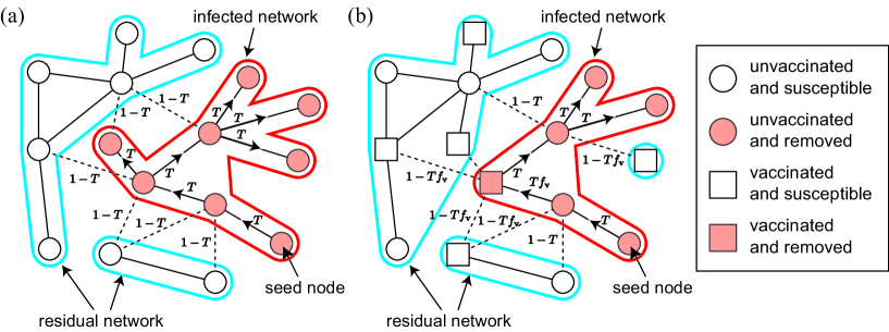
Figure 1: Propagating attack on networks (a) without and (b) with a defense strategy. $T$ and $Tf_{\rm v}$ are the probabilities that an infected (and eventually removed) node infects an unvaccinated and vaccinated neighbor in a propagating attack, respectively.

We adopt the SIR model, which is a continuous-time Markov process on a given static network with $N$ nodes, as the propagating attack. Each node takes one of the three states: susceptible, infected, and removed. All nodes except a randomly selected seed node are initially susceptible. The seed node is initially infected. Susceptible nodes get infected at a rate proportional to the number of infected neighbors. In other words, if a susceptible node is adjacent to an infected node, the susceptible node gets infected with probability $\beta\Delta t$ within short time $\Delta t$. An infected node becomes removed at a unit rate, i.e., with probability $\Delta t$ within short time $\Delta t$, irrespective of the neighbors’ states.

Following the methods employed in previous literature [31, 32], we analyze the bond percolation to estimate the transition points, the final size of global outbreaks, and that of residual networks of the SIR model. We assume that the disease is transmitted from an infected node to a susceptible node with probability $T=T(\beta)$, where $T=\int[1-\exp(-\beta\tau)]P(\tau)\rmd\tau$, $\tau$ is the infectious period during which the infected node is infected, and $P(\tau)$ is the distribution of $\tau$ [31, 32]. In other words, we map the SIR dynamics onto the bond percolation with open bond probability $T$. Strictly speaking, this mapping is not generally exact [33, 34, 35]. The transition point above which a global outbreak occurs and the mean final size of global outbreaks at a given $T$ obtained from the analysis of the bond percolation are precise for the SIR model. However, the bond percolation fails to predict the probability of global outbreaks in the SIR model [33, 34, 35]. The correspondence between the bond percolation and the SIR model is exact if the infectious period in the SIR model is assumed to be constant. When analyzing the effects of defense strategies (Sec. 3.2), we denote by $T_{i}$ the probability that susceptible node $i$ is infected by an infected neighbor. We set $T_{i}=T$ for all $i$ unless otherwise stated.

After a propagating attack, each node is either susceptible or removed (figure 1(a)). We call the network composed of removed nodes and that composed of susceptible nodes infected network and residual network, respectively. The infected network consists of a single component because an attack starts from a single seed. When $T$ is below a first transition point $T_{\rm c1}$, the size of the infected network is $o(N)$, whereas the residual network includes a giant component of order $O(N)$. When $T_{\rm c1}<T<T_{\rm c2}$, where $T_{\rm c2}$ is a second transition point, both the infected and residual networks have a giant component of order $O(N)$. When $T>T_{\rm c2}$, the giant component of the residual network is absent.

We consider two defense strategies. In the random defense, $Nf$ randomly selected nodes are vaccinated. In the degree-based defense, $Nf$ nodes with the largest degrees are vaccinated. We assume that $T_{i}$ decreases to $T_{i}=Tf_{\rm v}$ $(0\leq f_{\rm v}<1)$ for a vaccinated node $i$ (figure 1(b)). In epidemiology, the vaccine with $f_{\rm v}=0$ and that with $f_{\rm v}\neq 0$ are called perfect and leaky vaccination, respectively [22, 36].

3 Analysis

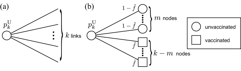
Figure 2: Schematics of (a) $F_{0}^{\rm U}(x)$, (b) $G_{0}^{\rm U}(x,y)$, (c) $P_{0}^{\rm U}(x,y)$, and (d) $P_{0}^{\rm V}(x,y)$.

3.1 SIR Model on Networks

In the following, we consider uncorrelated, locally tree-like networks with arbitrary degree distributions. In this section, we quickly review the derivation of $T_{\rm c1}$ and $T_{\rm c2}$ in the absence of a defense strategy [21, 31].

We denote by $p_{k}$ the fraction of nodes with degree $k$. We denote by $q_{k}$ the distribution of the excess degree defined as the degree of the node reached by following a randomly selected link minus 1; $q_{k}=(k+1)p_{k+1}/\langle k\rangle$, where $\langle\cdot\rangle$ represents the average of a quantity weighted by $p_{k}$. We define

$$F_{0}(x) \equiv\sum_{k}p_{k}x^{k},$$ (1)

$$F_{1}(x) \equiv\sum_{k}q_{k}x^{k}=\sum_{k}\frac{kp_{k}}{\langle k\rangle}x^{k-1}.$$ (2)

The giant component of the infected network is present if [21]

$$T>T_{\rm c1}=\frac{\langle k\rangle}{\langle k^{2}-k\rangle}.$$ (3)

To derive $T_{\rm c2}$, let $u$ be the probability that a node is not infected by a specific neighbor in a propagating attack. After a propagating attack, a node is susceptible with probability $\sum_{k}p_{k}u^{k}=F_{0}(u)$, and a node reached by following a link is susceptible with probability $\sum_{k}q_{k}u^{k}=F_{1}(u)$. The following recursive relationship determines $u$:

$$u=1-T+TF_{1}(u).$$ (4)

The probability that a node is susceptible in the residual network and its randomly selected neighbor is removed is equal to $(1-T)[1-F_{1}(u)]=u-F_{1}(u)$. Therefore, the probability that a node in the residual network has $m$ susceptible neighbors, i.e., the degree distribution of the residual network, is represented as

$$\frac{1}{F_{0}(u)}\sum_{k=m}^{\infty}p_{k}{k\choose m}F_{1}(u)^{m}[u-F_{1}(u)]^{k-m}.$$

The corresponding generating function $P_{0}(x)$ is given by

$$P_{0}(x) =\frac{1}{F_{0}(u)}\sum_{m=0}^{\infty}\sum_{k=m}^{\infty}p_{k}{k\choose m}F_{1}(u)^{m}[u-F_{1}(u)]^{k-m}x^{m}$$ (5)

$$=\frac{1}{F_{0}(u)}\sum_{k=0}^{\infty}p_{k}[F_{1}(u)(x-1)+u]^{k}=\frac{F_{0}[F_{1}(u)(x-1)+u]}{F_{0}(u)}.$$

Similarly, the generating function $P_{1}(x)$ for the excess degree distribution of the residual network is represented as

$$P_{1}(x)=\frac{F_{1}[F_{1}(u)(x-1)+u]}{F_{1}(u)}.$$ (6)

From Eq. (6), the mean excess degree of the residual network, denoted by $\langle k_{\rm ex}\rangle_{\rm res}$, is calculated as

$$\langle k_{\rm ex}\rangle_{\rm res}=\frac{\rmd}{\rmd x}P_{1}(x)\Big{|}_{x=1}=F_{1}^{\prime}(u).$$ (7)

The giant component of the residual network is absent if $T>T_{\rm c2}$, where $T_{\rm c2}$ is determined by $\langle k_{\rm ex}\rangle_{\rm res}=F_{1}^{\prime}(u)=1$ [21].

3.2 Defense strategies against propagating attacks

In the following, we calculate $T_{\rm c1}$ and $T_{\rm c2}$ in the presence of the random or degree-based defense.

3.2.1 Degree Distributions of Vaccinated and Unvaccinated Nodes in the Original Network

Under a defense strategy, each node is either unvaccinated (U) or vaccinated (V) (figure 1(b)). First, we derive the degree distribution of U nodes and that of V nodes in the original network. Under both defense strategies, a randomly selected node is U with probability $1-f$ and V otherwise. We denote the probability that a node reached by following a randomly selected link is a V node by $\tilde{f}$. Then, the probability that a node reached by following a randomly selected link is a U node is equal to $1-\tilde{f}$. Under the random defense, we obtain

$$\tilde{f}=f.$$ (8)

Under the degree-based defense, we obtain

$$\tilde{f}=\sum_{k=k_{\rm cut}}^{\infty}q_{k},$$ (9)

where $k_{\rm cut}$ is the minimum degree of V nodes determined by

$$\sum_{k=k_{\rm cut}}^{\infty}p_{k}=f.$$ (10)

Let $p_{k}^{\rm U}$ and $p_{k}^{\rm V}$ be the degree distributions of U nodes and V nodes, respectively, and $q_{k}^{\rm U}$ and $q_{k}^{\rm V}$ be the distributions of the excess degrees of U nodes and V nodes, respectively. For the random defense, we obtain

$$\{p_{k}^{\rm U},p_{k}^{\rm V}\} =\{p_{k},p_{k}\},$$ (11)

$$\{q_{k}^{\rm U},q_{k}^{\rm V}\} =\{q_{k},q_{k}\},$$ (12)

for all $k$. For the degree-based defense, we obtain

$$\{p_{k}^{\rm U},p_{k}^{\rm V}\}={\Biggl{\{}}\begin{array}[]{ccl}\{p_{k}/(1-f),0\}&\qquad(k<k_{\rm cut}),&\\ \{0,p_{k}/f\}&\qquad(k_{\rm cut}\leq k),&\end{array}$$ (15)

$$\{q_{k}^{\rm U},q_{k}^{\rm V}\}={\Biggl{\{}}\begin{array}[]{ccl}\{q_{k}/(1-\tilde{f}),0\}&\qquad(k<k_{\rm cut}),&\\ \{0,q_{k}/\tilde{f}\}&\qquad(k_{\rm cut}\leq k).&\end{array}$$ (18)

3.2.2 Derivation of $T_{\rm c1}$

We analyze the interaction of the generating functions for U nodes and those for V nodes. Related approaches have been adopted to analyze the percolation in networks that contain multiple types of nodes [37, 38]. We define the following generating functions

$$F_{0}^{\rm U}(x) \equiv\sum_{k=0}^{\infty}p_{k}^{\rm U}x^{k},$$ (19)

$$F_{0}^{\rm V}(x) \equiv\sum_{k=0}^{\infty}p_{k}^{\rm V}x^{k},$$ (20)

$$F_{1}^{\rm U}(x) \equiv\sum_{k=0}^{\infty}q_{k}^{\rm U}x^{k},$$ (21)

$$F_{1}^{\rm V}(x) \equiv\sum_{k=0}^{\infty}q_{k}^{\rm V}x^{k}.$$ (22)

A schematic of $F_{0}^{\rm U}(x)$ is shown in figure 2(a).

We extend the theory developed in [39] to derive $T_{\rm c1}$ for our model. Consider the mean number $N_{\ell}$ of removed nodes at distance $\ell$ from the seed node. We obtain

$$N_{\rm 1} =\sum_{k=0}^{\infty}p_{k}\sum_{m=0}^{k}{k\choose m}[mT+(k-m)Tf_{\rm v}](1-\tilde{f})^{m}\tilde{f}^{k-m}$$ (23)

$$=\Big{(}T\frac{\partial}{\partial x}+Tf_{\rm v}\frac{\partial}{\partial y}\Big{)}F_{0}[(1-\tilde{f})x+\tilde{f}y]\Big{|}_{x,y=1}=[T(1-\tilde{f})+Tf_{\rm v}\tilde{f}]F_{0}^{\prime}(1),$$

$$N_{\rm 2} =\sum_{k=0}^{\infty}p_{k}\sum_{m=0}^{k}{k\choose m}(1-\tilde{f})^{m}\tilde{f}^{k-m}$$ (24)

$$\quad\times\Big{\{}mT\sum_{k^{\prime}=0}^{\infty}q_{k^{\prime}}^{\rm U}\sum_{m^{\prime}=0}^{k^{\prime}}{k^{\prime}\choose m^{\prime}}[m^{\prime}T+(k^{\prime}-m^{\prime})Tf_{\rm v}](1-\tilde{f})^{m^{\prime}}\tilde{f}^{k^{\prime}-m^{\prime}}$$

$$\quad\quad+(k-m)Tf_{\rm v}\sum_{k^{\prime}=0}^{\infty}q_{k^{\prime}}^{\rm V}\sum_{m^{\prime}=0}^{k^{\prime}}{k^{\prime}\choose m^{\prime}}[m^{\prime}T+(k^{\prime}-m^{\prime})Tf_{\rm v}](1-\tilde{f})^{m^{\prime}}\tilde{f}^{k^{\prime}-m^{\prime}}\Big{\}}$$

$$=F_{0}^{\prime}(1)[T(1-\tilde{f})+Tf_{\rm v}\tilde{f}][T(1-\tilde{f}){F_{1}^{\rm U}}^{\prime}(1)+Tf_{\rm v}\tilde{f}{F_{1}^{\rm V}}^{\prime}(1)],$$

and

$$N_{\ell}=F_{0}^{\prime}(1)[T(1-\tilde{f})+Tf_{\rm v}\tilde{f}][T(1-\tilde{f}){F_{1}^{\rm U}}^{\prime}(1)+Tf_{\rm v}\tilde{f}{F_{1}^{\rm V}}^{\prime}(1)]^{\ell-1}=\Big{(}\frac{N_{2}}{N_{1}}\Big{)}^{\ell-1}N_{1},$$ (25)

for any $\ell\geq 1$. The infected network is a giant component if and only if $N_{2}>N_{1}$, or equivalently,

$$\frac{N_{2}}{N_{1}}=T(1-\tilde{f}){F_{1}^{\rm U}}^{\prime}(1)+Tf_{\rm v}\tilde{f}{F_{1}^{\rm V}}^{\prime}(1)>1.$$ (26)

Therefore, $T_{\rm c1}$ is determined from

$$T_{\rm c1}[(1-\tilde{f}){F_{1}^{\rm U}}^{\prime}(1)+f_{\rm v}\tilde{f}{F_{1}^{\rm V}}^{\prime}(1)]=1.$$ (27)

In the case of the random defense, where ${F_{1}^{\rm U}}^{\prime}(1)={F_{1}^{\rm V}}^{\prime}(1)=F_{1}^{\prime}(1)$ and $\tilde{f}=f$, Eq. (27) is reduced to

$$T_{\rm c1}[(1-f)+f_{\rm v}f]\frac{\langle k(k-1)\rangle}{\langle k\rangle}=1.$$ (28)

3.2.3 Derivation of $T_{\rm c2}$

The probability that a randomly selected U node has exactly $m$ U neighbors is equal to $\sum_{k=m}^{\infty}p_{k}^{\rm U}{k\choose m}(1-\tilde{f})^{m}\tilde{f}^{k-m}$. The generating function $G_{0}^{\rm U}(x,y)$ for this probability distribution, which is schematically shown in figure 2(b), is given by

$$G_{0}^{\rm U}(x,y)\equiv\sum_{k=0}^{\infty}p_{k}^{\rm U}\sum_{m=0}^{k}{k\choose m}(1-\tilde{f})^{m}\tilde{f}^{k-m}x^{m}y^{k-m}=F_{0}^{\rm U}[(1-\tilde{f})x+\tilde{f}y].$$ (29)

The generating function $G_{0}^{\rm V}(x,y)$ for the probability distribution that a $V$ node has $m$ U neighbors is given by

$$G_{0}^{\rm V}(x,y)\equiv\sum_{k=0}^{\infty}p_{k}^{\rm V}\sum_{m=0}^{k}{k\choose m}(1-\tilde{f})^{m}\tilde{f}^{k-m}x^{m}y^{k-m}=F_{0}^{\rm V}[(1-\tilde{f})x+\tilde{f}y].$$ (30)

Similarly, we obtain

$$G_{1}^{\rm U}(x,y)\equiv\sum_{k=0}^{\infty}q_{k}^{\rm U}\sum_{m=0}^{k}{k\choose m}(1-\tilde{f})^{m}\tilde{f}^{k-m}x^{m}y^{k-m}=F_{1}^{\rm U}[(1-\tilde{f})x+\tilde{f}y],$$ (31)

$$G_{1}^{\rm V}(x,y)\equiv\sum_{k=0}^{\infty}q_{k}^{\rm V}\sum_{m=0}^{k}{k\choose m}(1-\tilde{f})^{m}\tilde{f}^{k-m}x^{m}y^{k-m}=F_{1}^{\rm V}[(1-\tilde{f})x+\tilde{f}y].$$ (32)

Let $u_{\rm XY}$ ($X,Y\in\{U,V\}$) be the probability that an X node is not infected by a specific Y neighbor in a propagating attack. Then, a U node is susceptible with probability $G_{0}^{\rm U}(u_{\rm UU},u_{\rm UV})$, and a V node is susceptible with probability $G_{0}^{\rm V}(u_{\rm VU},u_{\rm VV})$. A U node connected to a randomly selected link is susceptible with probability $G_{1}^{\rm U}(u_{\rm UU},u_{\rm UV})$, and a V node connected to a random selected link is susceptible with probability $G_{1}^{\rm V}(u_{\rm VU},u_{\rm VV})$. Then, $u_{\rm UU}$, $u_{\rm UV}$, $u_{\rm VU}$, and $u_{\rm VV}$ satisfy the following recursive relationships:

$$u_{\rm UU} =1-T+TG_{1}^{\rm U}(u_{\rm UU},u_{\rm UV}),$$ (33)

$$u_{\rm UV} =1-T+TG_{1}^{\rm V}(u_{\rm VU},u_{\rm VV}),$$ (34)

$$u_{\rm VU} =1-Tf_{\rm v}+Tf_{\rm v}G_{1}^{\rm U}(u_{\rm UU},u_{\rm UV}),$$ (35)

$$u_{\rm VV} =1-Tf_{\rm v}+Tf_{\rm v}G_{1}^{\rm V}(u_{\rm VU},u_{\rm VV}).$$ (36)

To derive the degree distribution of U nodes in the residual network, consider a focal U node. When the focal U node is adjacent to a U node, the probability that the U neighbor is (infected and) eventually removed and the U focal node is not infected by this U neighbor in a propagating attack is equal to

$$(1-T)[1-G_{1}^{\rm U}(u_{\rm UU},u_{\rm UV})]=u_{\rm UU}-G_{1}^{\rm U}(u_{\rm UU},u_{\rm UV}).$$

When the focal U node is adjacent to a V node, the probability that the V neighbor is eventually removed and the focal U node is not infected by this V neighbor is equal to

$$(1-T)[1-G_{1}^{\rm V}(u_{\rm VU},u_{\rm VV})]=u_{\rm UV}-G_{1}^{\rm V}(u_{\rm VU},u_{\rm VV}).$$

Then, the probability that a U node has $m$ susceptible U neighbors and $n$ susceptible V neighbors and is not infected is equal to

$$\sum_{k=m+n}^{\infty}\sum_{m^{\prime}=m}^{k-n}p_{k}^{\rm U}{k\choose m^{\prime}}(1-\tilde{f})^{m^{\prime}}\tilde{f}^{k-m^{\prime}}{m^{\prime}\choose m}G_{1}^{\rm U}(u_{\rm UU},u_{\rm UV})^{m}[u_{\rm UU}-G_{1}^{\rm U}(u_{\rm UU},u_{\rm UV})]^{m^{\prime}-m}$$

$$\times{k-m^{\prime}\choose n}G_{1}^{\rm V}(u_{\rm VU},u_{\rm VV})^{n}[u_{\rm UV}-G_{1}^{\rm V}(u_{\rm VU},u_{\rm VV})]^{k-m^{\prime}-n}.$$

Therefore, the generating function $P_{0}^{\rm U}(x,y)$ for the degree distribution of U nodes in the residual network (figure 2(c)) is given by

$$P_{0}^{\rm U}(x,y) =\frac{1}{G_{0}^{\rm U}(u_{\rm UU},u_{\rm UV})}\sum_{k=0}^{\infty}p_{k}^{\rm U}\sum_{m^{\prime}=0}^{k}{k\choose m^{\prime}}(1-\tilde{f})^{m^{\prime}}\tilde{f}^{k-m^{\prime}}$$ (37)

$$\times\sum_{m=0}^{m^{\prime}}{m^{\prime}\choose m}G_{1}^{\rm U}(u_{\rm UU},u_{\rm UV})^{m}[u_{\rm UU}-G_{1}^{\rm U}(u_{\rm UU},u_{\rm UV})]^{m^{\prime}-m}x^{m}$$

$$\times\sum_{n=0}^{k-m^{\prime}}{k-m^{\prime}\choose n}G_{1}^{\rm V}(u_{\rm VU},u_{\rm VV})^{n}[u_{\rm UV}-G_{1}^{\rm V}(u_{\rm VU},u_{\rm VV})]^{k-m^{\prime}-n}y^{n}$$

$$=\frac{G_{0}^{\rm U}[G_{1}^{\rm U}(u_{\rm UU},u_{\rm UV})(x-1)+u_{\rm UU},G_{1}^{\rm V}(u_{\rm VU},u_{\rm VV})(y-1)+u_{\rm UV}]}{G_{0}^{\rm U}(u_{\rm UU},u_{\rm UV})}.$$

We can similarly derive the degree distribution of V nodes in the residual network. When a focal V node is adjacent to a U node, the probability that the U neighbor is eventually removed and the focal V node is not infected by this U neighbor is equal to

$$(1-Tf_{\rm v})[1-G_{1}^{\rm U}(u_{\rm UU},u_{\rm UV})]=u_{\rm VU}-G_{1}^{\rm U}(u_{\rm UU},u_{\rm UV}).$$

When the focal V node is adjacent to a V node, the probability that the V neighbor is eventually removed and the focal V node is not infected by this V neighbor is equal to

$$(1-Tf_{\rm v})[1-G_{1}^{\rm V}(u_{\rm VU},u_{\rm VV})]=u_{\rm VV}-G_{1}^{\rm V}(u_{\rm VU},u_{\rm VV}).$$

The generating function $P_{0}^{\rm V}(x,y)$ for the degree distribution of V nodes in the residual network (figure 2(d)) is given by

$$P_{0}^{\rm V}(x,y) =\frac{1}{G_{0}^{\rm V}(u_{\rm VU},u_{\rm VV})}\sum_{k=0}^{\infty}p_{k}^{\rm V}\sum_{m^{\prime}=0}^{k}{k\choose m^{\prime}}(1-\tilde{f})^{m^{\prime}}\tilde{f}^{k-m^{\prime}}$$ (38)

$$\times\sum_{m=0}^{m^{\prime}}{m^{\prime}\choose m}G_{1}^{\rm U}(u_{\rm UU},u_{\rm UV})^{m}[u_{\rm VU}-G_{1}^{\rm U}(u_{\rm UU},u_{\rm UV})]^{m^{\prime}-m}x^{m}$$

$$\times\sum_{n=0}^{k-m^{\prime}}{k-m^{\prime}\choose n}G_{1}^{\rm V}(u_{\rm VU},u_{\rm VV})^{n}[u_{\rm VV}-G_{1}^{\rm V}(u_{\rm VU},u_{\rm VV})]^{k-m^{\prime}-n}y^{n}$$

$$=\frac{G_{0}^{\rm V}[G_{1}^{\rm U}(u_{\rm UU},u_{\rm UV})(x-1)+u_{\rm VU},G_{1}^{\rm V}(u_{\rm VU},u_{\rm VV})(y-1)+u_{\rm VV}]}{G_{0}^{\rm V}(u_{\rm VU},u_{\rm VV})}.$$

Similarly, the generating functions for the excess degree distributions of U nodes and V nodes in the residual network are given by

$$P_{1}^{\rm U}(x,y)=\frac{G_{1}^{\rm U}[G_{1}^{\rm U}(u_{\rm UU},u_{\rm UV})(x-1)+u_{\rm UU},G_{1}^{\rm V}(u_{\rm VU},u_{\rm VV})(y-1)+u_{\rm UV}]}{G_{1}^{\rm U}(u_{\rm UU},u_{\rm UV})},$$ (39)

and

$$P_{1}^{\rm V}(x,y)=\frac{G_{1}^{\rm V}[G_{1}^{\rm U}(u_{\rm UU},u_{\rm UV})(x-1)+u_{\rm VU},G_{1}^{\rm V}(u_{\rm VU},u_{\rm VV})(y-1)+u_{\rm VV}]}{G_{1}^{\rm V}(u_{\rm VU},u_{\rm VV})},$$ (40)

respectively.

When we follow a randomly selected link in the residual network, we reach a U node with probability

$$\frac{(1-\tilde{f})G_{1}^{\rm U}(u_{\rm UU},u_{\rm UV})}{(1-\tilde{f})G_{1}^{\rm U}(u_{\rm UU},u_{\rm UV})+\tilde{f}G_{1}^{\rm V}(u_{\rm VU},u_{\rm VV})}.$$

Otherwise, we reach a V node. Then, the mean excess degree of the residual network is given by

$$\langle k_{\rm ex}\rangle_{\rm res} =\Big{(}\frac{\partial}{\partial x}+\frac{\partial}{\partial y}\Big{)}\frac{(1-\tilde{f})G_{1}^{\rm U}(u_{\rm UU},u_{\rm UV})P_{1}^{\rm U}(x,y)+\tilde{f}G_{1}^{\rm V}(u_{\rm VU},u_{\rm VV})P_{1}^{\rm V}(x,y)}{(1-\tilde{f})G_{1}^{\rm U}(u_{\rm UU},u_{\rm UV})+\tilde{f}G_{1}^{\rm V}(u_{\rm VU},u_{\rm VV})}\Big{|}_{x,y=1}$$ (41)

$$=(1-\tilde{f}){F_{1}^{\rm U}}^{\prime}[(1-\tilde{f})u_{\rm UU}+\tilde{f}u_{\rm UV}]+\tilde{f}{F_{1}^{\rm V}}^{\prime}[(1-\tilde{f})u_{\rm VU}+\tilde{f}u_{\rm VV}].$$

Because the second transition point is given by $\langle k_{\rm ex}\rangle_{\rm res}=1$, we find $T_{\rm c2}$ by solving

$$(1-\tilde{f}){F_{1}^{\rm U}}^{\prime}[(1-\tilde{f})u_{\rm UU}+\tilde{f}u_{\rm UV}]+\tilde{f}{F_{1}^{\rm V}}^{\prime}[(1-\tilde{f})u_{\rm VU}+\tilde{f}u_{\rm VV}]=1.$$ (42)

3.2.4 Component Size

The generating function formalism also gives the component size of the infected and residual networks. Because a randomly selected U node is susceptible with probability $G_{0}^{\rm U}(u_{\rm UU},u_{\rm UV})$ and a randomly selected V node is susceptible with probability $G_{0}^{\rm V}(u_{\rm VU},u_{\rm VV})$, the component size of the infected network $S_{\rm inf}$ is represented as

$$S_{\rm inf}=1-(1-f)G_{0}^{\rm U}(u_{\rm UU},u_{\rm UV})-fG_{0}^{\rm V}(u_{\rm VU},u_{\rm VV}).$$ (43)

To derive the largest component size of the residual network, we denote by $H_{0}^{\rm U}(x)$ and $H_{0}^{\rm V}(x)$ the generating functions for the size of the finite components of the residual networks to which a randomly selected U node and V node belong [3]. The average size $S_{\rm res}$ of the largest component of the residual network relative to the size of the original network is given by

$$S_{\rm res}=(1-S_{\rm inf})\left[1-\frac{G_{0}^{\rm U}(u_{\rm UU},u_{\rm UV})H_{0}^{\rm U}(1)+G_{0}^{\rm V}(u_{\rm VU},u_{\rm VV})H_{0}^{\rm V}(1)}{G_{0}^{\rm U}(u_{\rm UU},u_{\rm UV})+G_{0}^{\rm V}(u_{\rm VU},u_{\rm VV})}\right],$$ (44)

where

$$H_{0}^{\rm U}(1) =P_{0}^{\rm U}(A,B),$$ (45)

$$H_{0}^{\rm V}(1) =P_{0}^{\rm V}(A,B),$$ (46)

$$A \equiv H_{1}^{\rm U}(1)=P_{1}^{\rm U}(A,B),$$ (47)

$$B \equiv H_{1}^{\rm V}(1)=P_{1}^{\rm V}(A,B).$$ (48)

3.2.5 Degree-dependent Probability of Infection

We denote by $U(k)$ the probability that a node with degree $k$ is uninfected. Because a U node is susceptible with probability $G_{0}^{\rm U}(u_{\rm UU},u_{\rm UV})$ and a V node is susceptible with probability $G_{0}^{\rm V}(u_{\rm VU},u_{\rm VV})$, $U(k)$ is given by

$$\sum_{k=0}^{\infty}p_{k}U(k) =(1-f)G_{0}^{\rm U}(u_{\rm UU},u_{\rm UV})+fG_{0}^{\rm V}(u_{\rm VU},u_{\rm VV})$$ (49)

$$=(1-f)\sum_{k=0}^{\infty}p_{k}^{\rm U}[(1-\tilde{f})u_{\rm UU}+\tilde{f}u_{\rm UV}]^{k}+f\sum_{k=0}^{\infty}p_{k}^{\rm V}[(1-\tilde{f})u_{\rm VU}+\tilde{f}u_{\rm VV}]^{k}.$$

For the random defense, $p_{k}^{\rm U}$ and $p_{k}^{\rm V}$ are given by Eq. (11). Therefore, Eq. (49) is reduced to

$$\sum_{k=0}^{\infty}p_{k}U(k)=\sum_{k=0}^{\infty}p_{k}\{(1-f)[(1-f)u_{\rm UU}+fu_{\rm UV}]^{k}+f[(1-f)u_{\rm VU}+fu_{\rm VV}]^{k}\}.$$ (50)

Because Eq. (50) is satisfied for an arbitrary degree distribution $\{p_{k}\}$, we obtain

$$U(k)=(1-f)[(1-f)u_{\rm UU}+fu_{\rm UV}]^{k}+f[(1-f)u_{\rm VU}+fu_{\rm VV}]^{k}.$$ (51)

For the degree-based defense, $p_{k}^{\rm U}$ and $p_{k}^{\rm V}$ are given by Eq. (LABEL:pktarget). Therefore, Eq. (49) is reduced to

$$\sum_{k=0}^{\infty}p_{k}U(k)=\sum_{k=0}^{k_{\rm cut}-1}p_{k}[(1-\tilde{f})u_{\rm UU}+\tilde{f}u_{\rm UV}]^{k}+\sum_{k=k_{\rm cut}}^{\infty}p_{k}[(1-\tilde{f})u_{\rm VU}+\tilde{f}u_{\rm VV}]^{k}.$$ (52)

Because Eq. (52) is satisfied for arbitrary $\{p_{k}\}$, we obtain

$$U(k)={\Biggl{\{}}\begin{array}[]{ccl}[(1-\tilde{f})u_{\rm UU}+\tilde{f}u_{\rm UV}]^{k}&\qquad(k<k_{\rm cut}),&\\ [(1-\tilde{f})u_{\rm VU}+\tilde{f}u_{\rm VV}]^{k}&\qquad(k_{\rm cut}\leq k).&\end{array}$$ (55)

4 Numerical Results

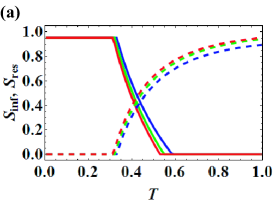
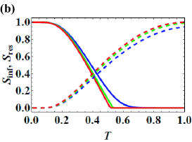
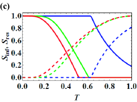
Figure 3: Component size $S_{\rm inf}$ of the infected network (dashed lines) and the largest component size $S_{\rm res}$ of the residual network (solid lines) for (a) random graph with the random defense (case (i)), (b) SF network with the random defense (case (ii)), and (c) SF network with the degree-based defense (case (iii)). We set $f=0.05$. The different lines correspond to $f_{\rm v}=0.00$, $0.50$, and $1.00$, from right to left.

On the basis of the theoretical results obtained in Sec. 3, we numerically examine the robustnesses of different networks against the propagating attack. We consider the following three combinations of networks and defense strategies:

(i)

random graph with random defense,

(ii)

uncorrelated SF network with random defense, and

(iii)

uncorrelated SF network with degree-based defense.

We assume that the SF network has degree distribution $p_{k}\propto k^{-3}$, where $k\geq k_{\rm min}\equiv 2$, which yields $\langle k\rangle\simeq 3.19$. For a fair comparison, we assume that $\langle k\rangle$ of the random graph is equal to that of the SF network. For the random graph, we obtain $F_{0}(x)=F_{1}(x)=\exp[\langle k\rangle(x-1)]$. For the SF network, we obtain $F_{0}(x)=\sum_{k=0}^{\infty}p_{k}x^{k}={\rm Li}_{3}(x)/{\rm Li}_{3}(1)$, $F_{1}(x)=\sum_{k=0}^{\infty}kp_{k}x^{k-1}/\sum_{k=0}^{\infty}kp_{k}={\rm Li}_{2}(x)/x{\rm Li}_{2}(1)$, where ${\rm Li}_{n}(x)$ is the $n$th polylogarithm of $x$, i.e., ${\rm Li}_{n}(x)\equiv\sum_{k=1}^{\infty}x^{k}k^{-n}$. In the random defense (cases (i) and (ii)), $F_{0}^{\rm U}(x)=F_{0}^{\rm V}(x)=F_{0}(x)$ and $F_{1}^{\rm U}(x)=F_{1}^{\rm V}(x)=F_{1}(x)$. In the degree-based defense (case (iii)), we vaccinate all the nodes whose degree is equal to or larger than $k_{\rm cut}$ such that the fraction of V nodes does not exceed $f$. Then, we vaccinate some nodes with degree $k_{\rm cut}-1$ such that the total fraction of V nodes is equal to $f$. The other nodes with degree $k_{\rm cut}-1$ are U nodes. The generating functions for U and V nodes are given by

$$F_{0}^{\rm U}(x) =\sum_{k=0}^{k_{\rm cut}^{\prime}}p_{k}x^{k}-Cp_{k_{\rm cut}^{\prime}}x^{k_{\rm cut}^{\prime}},$$ (56)

$$F_{1}^{\rm U}(x) =\sum_{k=0}^{k_{\rm cut}^{\prime}}q_{k}x^{k}-Cq_{k_{\rm cut}^{\prime}}x^{k_{\rm cut}^{\prime}},$$ (57)

$$F_{0}^{\rm V}(x) =\sum_{k=k_{\rm cut}}^{\infty}p_{k}x^{k}+Cp_{k_{\rm cut}^{\prime}}x^{k_{\rm cut}^{\prime}},$$ (58)

$$F_{1}^{\rm V}(x) =\sum_{k=k_{\rm cut}}^{\infty}q_{k}x^{k}+Cq_{k_{\rm cut}^{\prime}}x^{k_{\rm cut}^{\prime}},$$ (59)

where $C=(f-\sum_{k=k_{\rm cut}}^{\infty}p_{k})/p_{k_{\rm cut}^{\prime}}$ and $k_{\rm cut}^{\prime}=k_{\rm cut}-1$. For each case, we apply the results of Sec. 3.2 to obtain the component sizes and transition points. For given $f$ and $f_{\rm v}$, we substitute $F_{0}^{\rm U}(x)$, $F_{1}^{\rm U}(x)$, $F_{0}^{\rm V}(x)$, and $F_{1}^{\rm V}(x)$ in Eq. (27) to obtain $T_{\rm c1}$. We also substitute $F_{0}^{\rm U}(x)$, $F_{1}^{\rm U}(x)$, $F_{0}^{\rm V}(x)$, and $F_{1}^{\rm V}(x)$ in Eqs. (33)–(36) to determine $u_{\rm UU}$, $u_{\rm UV}$, $u_{\rm VU}$, and $u_{\rm VV}$. Then, we use the obtained values of $u_{\rm UU}$, $u_{\rm UV}$, $u_{\rm VU}$, and $u_{\rm VV}$ to derive $T_{\rm c2}$, $S_{\rm inf}$, and $S_{\rm ref}$ from Eqs. (42), (43), and (44), respectively.

We first examine the component sizes $S_{\rm inf}$ of the infected network and $S_{\rm res}$ of the residual network using Eqs. (43) and (44). The results for case (i) with $f=0.05$ are shown in figure 3(a). When $T$ is small, $S_{\rm inf}=0$ (in the limit of the infinite network size) holds true irrespective of the value of $f_{\rm v}$, as shown by different dashed lines in figure 3(a). When $T>T_{\rm c1}\approx 0.33$, $S_{\rm inf}$ increases and $S_{\rm res}$ decreases with an increase in $T$. When $T>T_{\rm c2}\approx 0.6$, we obtain $S_{\rm res}=0$. The precise values of $T_{\rm c1}$ and $T_{\rm c2}$ vary with $f_{\rm v}$. Efficient vaccines (i.e., small $f_{\rm v}$) make $S_{\rm inf}$ small and $S_{\rm res}$ large and increase $T_{\rm c1}$ and $T_{\rm c2}$.

The results for case (ii) are shown in figure 3(b). $T_{\rm c1}$ is much smaller than in case (i); Eq. (28) implies $T_{\rm c1}=0$ when ${F_{1}^{\rm V}}^{\prime}(1)$ diverges. For $f_{\rm v}\neq 0$, $S_{\rm res}$ behaves qualitatively the same as that for case (i). In particular, the value of $T_{\rm c2}$ for $f_{\rm v}=1$ is only slightly smaller than that for case (i). For $f_{\rm v}=0$, $S_{\rm res}$ behaves differently; $S_{\rm res}>0$ even when $T=1$, implying that the residual network is never destroyed.

The results for case (iii) are shown in figure 3(c). We find that the degree-based defense is effective at decreasing (increasing) $S_{\rm inf}$ ($S_{\rm res}$) as compared with the random defense (case (ii)). In particular, the perfect vaccines (i.e., $f_{\rm v}=0$) contain the propagating attack when $T<T_{\rm c1}\approx 0.63$. We find from Eq. (27) that $T_{\rm c1}\neq 0$ only for $f_{\rm v}=0$. Therefore, any leaky vaccination (i.e., $f_{\rm v}>0$) fails to contain the attack because ${F_{1}^{\rm V}}^{\prime}(1)$ diverges. We remark that, for $f_{\rm v}=0$, Eq. (27) is reduced to a known result [26]

$$T_{\rm c1}\sum_{k=0}^{k_{\rm cut}-1}\frac{k(k-1)}{\langle k\rangle}p_{k}=1.$$ (60)

We also remark that, for $f_{\rm v}=1$, the value of $T_{\rm c2}$ coincides with that for case (ii) as expected; the effect of vaccination is completely null when $f_{\rm v}=1$.

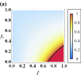
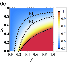
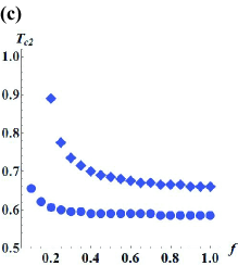
Figure 4: Results for the random graph with the random defense (case (i)). (a) $T_{\rm c1}$ and (b) $T_{\rm c2}$ as functions of $f$ and $f_{\rm v}$. The solid lines indicate $T_{\rm c1}=1$ in (a) and $T_{\rm c2}=1$ in (b). The dashed lines indicate $f(1-f_{\rm v})=0.1$ and $f(1-f_{\rm v})=0.2$. (c) $T_{\rm c2}$ conditioned by $f(1-f_{\rm v})=0.1$ (circles) and $0.2$ (diamonds).

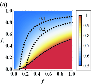
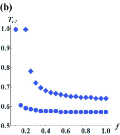
Figure 5: Results for the SF network with random defense (case (ii)). (a) $T_{\rm c2}$ as a function of $f$ and $f_{\rm v}$. The solid line indicates $T_{\rm c2}=1$. The dashed lines indicate $f(1-f_{\rm v})=0.1$ and $f(1-f_{\rm v})=0.2$. (b) $T_{\rm c2}$ conditioned by $f(1-f_{\rm v})=0.1$ (circles) and $0.2$ (diamonds).

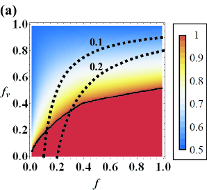
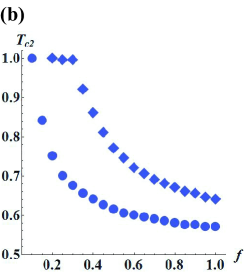
Figure 6: Results for the SF network with the degree-based defense (case (iii)). (a) $T_{\rm c2}$ as a function of $f$ and $f_{\rm v}$. The solid line indicates $T_{\rm c2}=1$. The dashed lines indicate $f(1-f_{\rm v})=0.1$ and $f(1-f_{\rm v})=0.2$. (b) $T_{\rm c2}$ conditioned by $f(1-f_{\rm v})=0.1$ (circles) and $0.2$ (diamonds).

In figures 4, 5, and 6, $T_{\rm c1}$ and $T_{\rm c2}$ obtained from Eqs. (27) and (42) are shown for the three cases.

$T_{\rm c1}$ monotonically increases with $f$ and monotonically decreases with $f_{\rm v}$ in case (i) (figure 4(a)). When $T_{\rm c1}=1$ (the red region bounded by the bold line in figure 4(a)), a global infection does not occur at any infection rate. On the basis of Eq. (27), the boundary of the region $T_{\rm c1}=1$ is given by

$$1-f+f_{\rm v}f=\frac{\langle k\rangle}{\langle k(k-1)\rangle}.$$ (61)

In case (ii), $T_{\rm c1}=0$ for any $f$ and $f_{\rm v}$ unless $(f,f_{\rm v})=(1,0)$. In case (iii), $T_{\rm c1}=0$ if $f_{\rm v}>0$ or $(f,f_{\rm v})=(0,0)$ for the following reason. If $f_{\rm v}>0$, ${F_{1}^{\rm V}}^{\prime}(1)$ in Eq. (26) diverges. If $f=0$, ${F_{1}^{\rm U}}^{\prime}(1)$ in Eq. (26) diverges (and ${F_{1}^{\rm V}}^{\prime}(1)=0$).

Similar to $T_{\rm c1}$, $T_{\rm c2}$ monotonically increases with $f$ and monotonically decreases with $f_{\rm v}$ in all the cases (figures 4(b), 5(a), and 6(a)). When $T_{\rm c2}=1$, the residual network is not disintegrated at any infection rate (the red regions bounded by the bold line in figures 4(b), 5(a), and 6(a)).

When $f_{\rm v}=0$, the SF network yields $T_{\rm c2}=1$ for any $f>0$, either for the random defense (figure 5(a)) and the degree-based defense (figure 6(a)). In this situation, V nodes are never infected such that they percolate in a SF network. This phenomenon is identical to the standard site percolation on SF networks with $\gamma\leq 3$; randomly located nodes percolate even at an infinitesimally small occupation probability [10, 11].

The comparison of the values of $T_{\rm c2}$ among the three cases based on figures 4(b), 5(a), and 6(a) suggests the following. When the vaccines are not efficient (i.e., $f_{\rm v}\sim 1$), the network is the most robust for case (i) among the three cases in the sense that $T_{\rm c2}$ is the largest. In this situation, $T_{\rm c2}$ for the SF network is slightly smaller than that for the random graph (also see figure 3). When $f_{\rm v}$ takes an intermediate value, the network is the most robust for case (iii). The network is the most fragile for case (ii) except for fairly small $f_{\rm v}$ and $f$, in which case the residual network mainly composed of vaccinated nodes can percolate on the SF network and not on the random graph.

In reality, there may be a trade-off between the required number of vaccines and the efficiency of vaccines. Therefore, we measure $T_{\rm c2}$ under the constraints $f(1-f_{\rm v})=0.1$ and $f(1-f_{\rm v})=0.2$; $f$ and $1-f_{\rm v}$ represent the number and efficiency of vaccines, respectively. As shown in figures 4(c), 5(b), and 6(b), the network becomes progressively robust as $f$ decreases (i.e., small number of vaccines) and $f_{\rm v}$ decreases (i.e., high efficiency of vaccines) in all the three cases.

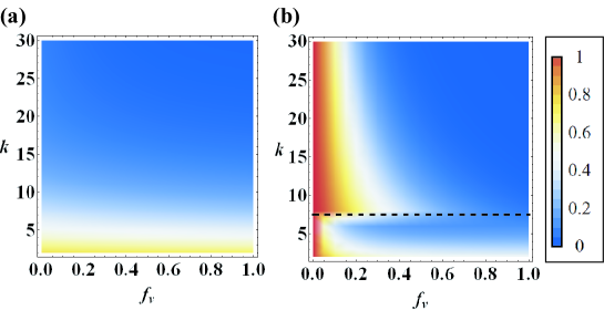
Figure 7: Probability $U(k)$ that a node with degree $k$ in the SF network is uninfected. (a) Random defense (case (ii)). (b) Degree-based defense (case (iii)). We set $T_{0}=0.4$ and $f=0.05$. The dashed line in (b) indicates $k_{\rm cut}=8$.

The difference between the random and degree-based defenses in the SF network is apparent when we look at $U(k)$, i.e., the probability that a node with degree $k$ remains uninfected. In figures 7(a) and 7(b), $U(k)$ values are shown for cases (ii) (Eq. (51)) and (iii) (Eq. (55)), respectively. As expected, the degree-based defense cuts down the probability of infection for nodes with high degrees, whereas the random defense does not. Furthermore, the indirect effect of vaccines, i.e., the suppression of the infection probability for U nodes, is strong under the degree-based defense. For example, some fractions of U nodes with degree $k<k_{\rm cut}$ (below the dashed line in figure 7 (b)) remain uninfected.

5 Summary

We investigated the effect of defense strategies on the robustness of networks against propagating attacks by extending the generating function framework developed by Newman [21]. In particular, under vaccination strategies, we analytically obtained the second critical infection rate above which the residual network is disintegrated. We applied the analytical results to the three cases: the random graph with the random defense, the SF network with the random defense, and the SF network with the degree-based defense. The first critical point of the SF network depends crucially on whether the effect of the vaccines is perfect or leaky. Even under the degree-based defense, the leaky vaccines cannot prevent a global outbreak on heterogeneous networks. We also found that, under a trade-off between the number and efficiency of vaccines, it is better to administer a small number of vaccines with high efficiency than vice versa to prevent the residual network from being disintegrated.

Reference

References

- [1] Barabási A -L and Albert R 1999 Science 286 509.
- [2] Albert R and Barabási A -L, 2002 Rev. Mod. Phys. 74 47–97.
- [3] Newman M E J, 2003 SIAM Rev. 45 167–256.
- [4] Boccaletti S, Latora V, Moreno Y, Chavez M, and Hwang D U, 2006 Phys. Rep. 424 175.
- [5] Dorogovtsev S N, Goltsev A V, and Mendes J F F, 2008 Rev. Mod. Phys.80 1275–1335.
- [6] Barrat A, Barthélemy M, and Vespignani A, 2008 Dynamical processes on complex networks (Cambridge: Cambridge University Press).
- [7] Newman M E J, 2010 Networks: An Introduction (Oxford: Oxford Univeristy Press).
- [8] Cohen R and Havlin S, 2010 Complex Networks: Structure, Robustness and Function (Cambridge: Cambridge University Press).
- [9] Albert R, Jeong H, and Barabási A -L, 2000 Nature 406 378–382.
- [10] Callaway D S, Newman M E J, Strogatz S H, and Watts D J, 2000 Phys. Rev. Lett. 85 5468–5471.
- [11] Cohen R, Erez K, ben-Avraham D, and Havlin S, 2000 Phys. Rev. Lett. 85 4626–4628.
- [12] Cohen R, Erez K, ben-Avraham D, and Havlin S, 2001 Phys. Rev. Lett. 86 3682–3685.
- [13] Holme P, Kim B J, Yoon C N, and Han S K, 2002 Phys. Rev.E 65 056109.
- [14] Gallos L K, Cohen R, Argyrakis P, Bunde A, and Havlin S, 2005 Phys. Rev. Lett. 94 188701.
- [15] Kephart J O and White S R, 1991 Proc. of the 1991 IEEE Computer Society Symp. on Research in Security and Privacy pp 343–359.
- [16] Kephart J O and White S R, 1993 Proc. of the 1993 IEEE Computer Society Symp. on Research in Security and Privacy pp 2–15.
- [17] Pastor-Satorras R and Vespignani A, 2001 Phys. Rev. Lett. 86 3200–3203.
- [18] Pastor-Satorras R and Vespignani A, 2001 Phys. Rev.E 63 066117.
- [19] Moreno Y, Pastor-Satorras R, and Vespignani A, 2002 Eur. Phys. J.B 26 521–529.
- [20] Castellano C and Pastor-Satorras R, 2010 Phys. Rev. Lett. 105 218701.
- [21] Newman M E J, 2005 Phys. Rev. Lett. 95 108701.
- [22] Bansal S and Meyers L A, The impact of past epidemics on future disease dynamics, 2009 arXiv:0910.2008.
- [23] Bansal S, Pourbohloul B, Hupert N, Grenfell B, and Meyers L A, 2010 PLoS ONE 5 e9360.
- [24] Funk S and Jansen V A A, 2010 Phys. Rev.E 81 036118.
- [25] Pastor-Satorras R and Vespignani A, 2002 Phys. Rev.E 65 036104.
- [26] Madar N, Kalisky T, Cohen R, ben-Avraham D, and Havlin S, 2004 Eur. Phys. J.B 38 269–276.
- [27] Cohen R, Havlin S, and ben-Avraham D, 2003 Phys. Rev. Lett. 91 247901.
- [28] Holme P, 2004 Europhys. Lett. 68 908.
- [29] Gallos L K, Liljeros F, Argyrakis P, Bunde A, and Havlin S, 2007 Phys. Rev.E 75 045104.
- [30] Chen Y, Paul G, Havlin S, Liljeros F, and Stanley H E, 2008 Phys. Rev. Lett. 101 058701.
- [31] Newman M E J, 2002 Phys. Rev.E 66 016128.
- [32] Grassberger P, 1983 Math. Biosci. 63 157–172.
- [33] Kenah E and Robins J M, 2007 Phys. Rev.E 76 036113.
- [34] Miller J C, 2007 Phys. Rev.E 76 010101.
- [35] Kenah E and Miller J C, 2011 Interdisciplinary Perspectives on Infectious Diseases 2011 543520.
- [36] Halloran M E, Haber M, and Longini I M, 1992 Am. J. Epidemiol. 136 328–343.
- [37] Söderberg B, 2002 Phys. Rev.E 66 066121.
- [38] Leicht E A and D’Souza R M, Percolation on interacting networks, 2009 arXiv:0907.0894 [cond-mat].
- [39] Newman M E J, Random graphs as models of networks, 2002 arXiv:cond-mat/0202208.