Low energy modes and Debye behavior in a colloidal crystal

Abstract

We study the vibrational spectrum and the low energy modes of a three dimensional colloidal crystal using confocal microscopy. This is done in a two-dimensional cut through a three-dimensional crystal. We find that the observed density of states is incompatible with the standard Debye form in either two or three dimensions. These results are confirmed by numerical simulations. We show that an effective theory for the projections of the modes onto the two-dimensional cut describes the experimental and simulation data in a satisfactory way.

, , ,, ,

1 Introduction

Colloidal particles dispersed in a solvent form fluid and solid phases under appropriate conditions [1, 2]. The ordered phase is interesting due to their long-range order combined with very soft mechanical properties making thermal fluctuations very important. For the colloidal systems considered here, the shear modulus is only a few $Pa$, whereas crystalline solids typically have moduli in the $GPa$ range[3, 4]. Comparison of the properties of colloidal systems with harder molecular solids is a matter of ongoing research [5, 6, 7]. Earlier studies have largely focused on the the phonon dispersion behavior measured by means of video microscopy [5] or light scattering [8, 9]. However, to our knowledge there is no experiment that directly verifies the Debye scaling in the measured density of states of the vibrational modes. Even for molecular crystals, the this has proven rather hard to measure directly; mostly neutron scattering experiments have provided some but not much data that agree with the expected $\omega^{2}$ behavior [10]. Perhaps for this reason the temperature dependence of the specific heat is usually taken as the hallmark for the Debye behavior of normal crystalline solids. The question we ask in this paper is how the spectrum measured in a colloidal crystal compares with the predicted Debye behavior, $D(\omega)\sim\omega^{d-1}$.
To study the energy spectrum, we calculate the normal modes of a hard sphere colloidal crystal from the correlations in particle displacements. The colloidal particles used are small enough so that they perform small ‘vibrations’ in response to the thermal excitations of the surroundings. We use confocal microscopy to observe and record these particle motions in a two dimensional field of view. The eigenvalues of the dynamical matrix and normal modes are then obtained from the spatial correlations [5, 11]of the measured displacements. The present experimental results are compared and complemented with a simplified continuum theory as well as Monte Carlo simulation of hard sphere crystals. The main conclusion is that the spectrum of slice of a three dimensional system has a anomalous density of states which varies as $D(\omega)\sim\omega^{3}$, which contrasts the assumption made in [12] that a $2d$ cut should exhibit the expecred $3d$ Debye behavior. However our experimental results do agree with simulations presented below, and can in addition be explained by a simplified continuum theory.

1.1 Experiments

Hard sphere colloidal systems undergo phase changes with the volume fraction $\phi$ as control parameter. There is no liquid-gas transition, but fluid-solid coexistence [1, 2] is observed from the freezing transition point $\phi_{f}=0.494$ until the melting point $\phi_{m}=0.545$. A stable crystalline phase exists above $0.545$ until the closed packed density at $\phi=0.74$. The colloids we use are charge stabilized PMMA particles with a diameter of $a=1.3\mu m$ with a very small size polydispersity of about $2\%$. The particles are dyed with rhodamine and are suspended in a CHB (cyclohexyl bromide) / decalin mixture which closely matches both the density and the index of refraction of the particles. We further add organic salt TBAB (tetrabutylammoniumbromide) to screen any possible residual charges.

Figure 1: Snapshot of a two dimensional section in a field of view of $60\mu m\times 60\mu m$ with a hexagonal symmetry.

The crystal was grown in a sample cell made of parallel plates with a confinement of approximately $\sim 1mm$ along the vertical direction. The volume fraction of the present colloidal crystal is about $\phi\approx 0.57$. Using confocal microscopy we acquire images at a speed of $25$ frames per second of a two dimensional section of about 60 $\mu m$ x 60 $\mu m$ of the larger three dimensional crystal. The 2D slice was taken at a distance of $25-30$ micron away from the coverslip, deep enough to avoid the effects of confinement. The entire crystal is polycrystalline, but we take our data from a region of the crystal that as far as we can see is perfectly crystalline and contains no defects. The particle positions are identified and tracked for a period of about $120$ seconds using standard particle-tracking software; this results in a total of $3000$ frames. Fig. 1 shows a typical snapshot of a two dimensional section of the measured crystal.

1.2 Density of states

We obtain an ensemble of projected particle positions ${r}_{i}=\{x_{i},y_{i}\}$ from the above measurements. The displacement components from the mean position for the $i^{th}$ particle is given by,

$$u_{\mu}(i)=r_{\mu i}-\langle r_{\mu i}\rangle.$$ (1)

$$u_{\nu}(i)=r_{\nu i}-\langle r_{\nu i}\rangle.$$

where $\mu,\nu=x,y$ and “$\langle\rangle$” indicates an ensemble average. The $k^{th}$ Fourier component of the above displacements is given by,

$$u_{\mu}(k)=\sum_{i=1}^{N}u_{\mu}(\vec{r_{i}})exp(-j\vec{k}.\vec{r_{i}})$$ (2)

$$u_{\nu}(k)=\sum_{i=1}^{N}u_{\nu}(\vec{r_{i}})exp(-j\vec{k}.\vec{r_{i}}),k=\{k_{x},k_{y}\}$$

The summation above runs over all the $N=1386$ colloidal particles present in the system and the respective $k$ values are chosen from the first Brillouin zone of the experimental lattice.

Figure 2: Left: Density of states as obtained from the correlations, eq. 4. Right: The dispersion curves of transverse and longitudinal vibrations. The frequencies (vertical axis) near the zone boundary where $d\omega/dk\approx 0$ coincide with the positions of the singularities (peaks) in the density of states on top.

Now, the potential energy of a harmonic crystal can be written as,

$$U=1/2\sum_{k}(u^{*}_{\mu}(k)K_{\mu\nu}(k)u_{\nu}(k))$$ (3)

where $K_{\mu\nu}(k)$ [5]is the $2\times 2$ dynamical matrix in Fourier space. From equipartition each of the above quadratic terms $u^{*}_{\mu}(k)K_{\mu\nu}(k)u_{\nu}(k)/2$ contains an energy of $k_{B}T/2$. Therefore we can write,

$$K^{-1}_{\mu\nu}(k)=\left\langle{u}^{*}_{\mu}(k){u}_{\nu}(k)\right\rangle/k_{B}T.$$ (4)

In the present study, we take our two-dimensional data and analyse it according to the above scheme. The mode frequencies of the system are related to the eigenvalues $\lambda$ of the matrix $K_{\mu\nu}^{-1}(k)$ as,

$$\omega(k)=\sqrt{1/\lambda(k)}.$$ (5)

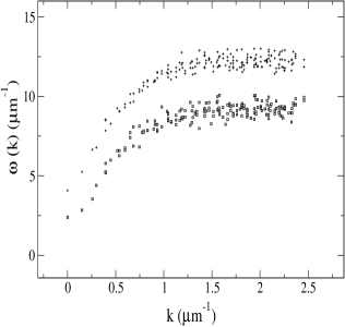
Now, there are $N$ of such $2\times 2$ matrices ($K_{\mu\nu}^{-1}$) corresponding to the number $N$ of $k$ values. Separate diagonalization of each of these gives us $2N$ normal mode frequencies. Each of the $N$ branches of frequencies as a function of $k$ then leads to the two dispersion curves shown in Fig. 2. The density of states $D(\omega)$ as obtained from these frequencies is shown in the same figure. A two peak structure is apparent in the density of states. Such peaks are familiar from the theory of lattice dynamics and often signal van Hove singularities [10] occurring due to the vanishing group velocities $\nabla_{k}\omega$ at certain wave vectors. Indeed we see that the frequencies where $d\omega/dk\approx 0$ (close the zone boundary) on the dispersion curves coincide with the ones around which peaks appear in the density of states.

One important additional remark is that if we make the reasonable assumption that the system is in local equilibrium, the values of the squared-displacements are independent of the dynamics, which may be overdamped or purely ballistic, and even contain hydrodynamic interactions. What depends on the nature of the dynamics is the actual time-dependence of the displacements, but not their statistical distribution. Our new method [11, 14] directly analyzes the normal modes of the vibrations in the cages from the displacement correlations. If the system were harmonic, undamped and without hydrodynamic interactions, the DOS obtained from e.g Fourier transforming the velocity autocorrelation function and our method would coincide. However, in the former method all the spatial in- formation is lost. The strength of the present analysis using confocal measurements lies in directly visualizing the collective modes at low spatial frequencies and therefore gaining information about the nature of such modes. But the price to pay for this is the exclusion of knowledge of damping, anharmonicity and hydrodynamic interactions.

1.3 Visualization of modes

The next question we ask is what the low energy modes of the above system look like ? To be able to visualize these modes we compute the spatial correlation between the particles in real space via the covariance matrix.

a

b

c

Figure 3: Tomography of the normal modes shown in a field of view of $60\mu m\times 60\mu m$. The pictures correspond to increasing frequencies going from a) to b) to c). The very low frequency ones show the extended plane wave nature of the modes. This coherent character is lost and modes appears to be random as higher frequencies are approached.

This matrix, which has been used recently in studying normal mode properties of colloidal [5, 13, 12, 11, 14] and granular systems [15], is defined as:

$$Q_{\mu\nu}(i,j)=\left\langle u_{\mu}(i))u_{\nu}(j)\right\rangle.$$ (6)

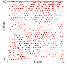
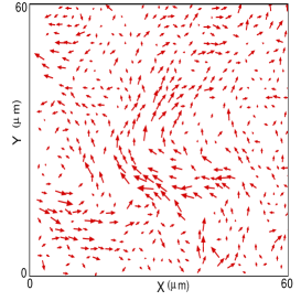
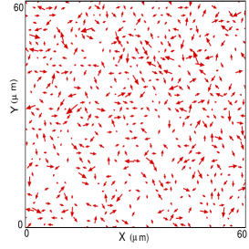
This is a $2N\times 2N$ dimensional matrix for $N$ particles. Any eigenvector $\{v_{l}\}$ of the above matrix represents a normal mode at a single “frequency” $\omega_{l}=\sqrt{1/\lambda_{l}}$. In our colloidal system, it allows us to compute the normal modes, rather than supposing plane waves as in eq. (4). A few examples of the normal modes are shown in Fig. (3). The modes in the low-frequency part of the spectrum show a clearly coherent motion extending over large part of the field of view. For higher frequencies the modes appears to be rather random in nature.

1.4 Scaling of the low frequency density of states

Having described the vibrational spectrum of the experimental crystal we come back to one of the central questions of this paper, which is what happens if one tries to study the matrix eq. (4) using only a subset of the particles of the true three dimensional system, in particular if one reconstructs the dynamical matrix from the measurements from a single plane within the sample as we do. What is the nature of the effective interactions found in the analysis and what is the density of states found in the two-dimensional slice ?

Figure 4: A power-law fit to the low frequency part of the cumulative density of states $N(\omega)$. The measured exponent $(N(\omega)\sim\omega^{\alpha})$, is $\alpha\approx 3.93\pm 0.19$.

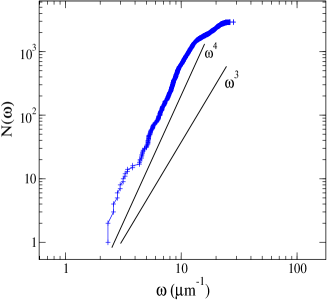
To answer this we look at how the measured cumulative density of states of the colloidal crystal compares to the expected integrated density of states $N(\omega)=\int D(\omega)d\omega\sim\omega^{3}$ in $d=3$ We find that the measured $N(\omega)$ scales approximately as $\omega^{4}$ rather than $\omega^{3}$. We fit the integrated density of states to a power law with adjustable exponent, $\alpha$. Our data best fits to a value close to $\alpha=3.9+/-0.19$, far from the expected value $\alpha=3$ for a three dimensional elastic medium and even further from the value $\alpha=2$ expected in two dimensions. The quoted error is the one-sigma deviation of the Gaussian distribution of the scatter of the data around the fit. A standard error calculation gives that the $99$ percent probability interval is $3.93+/-0.416$, excluding the power $3$. Furthermore, we have done a few different measurement series on the same sample, but at different locations within the sample and size of the region probed. Each of these measurements was analyzed separately to ensure the robustness and consistency of the results. Taking data from different regions in the sample, the exponent was found to always lie in the interval $[3.7-4.1]$, with a mean value of $3.9$. This again confirms the value of the exponent and its error quoted above.

The above scaling of the low frequency cumulative DOS is also checked with the spectrum from the spatial covariance matrix that contains the non-diagonal correlations(sec.2.1). This yields an exponent of about $3.6+/-0.3$ which is reasonably close to the scaling $(3.93+/-0.19)$. Thus, within the experimental error, the scaling of the DOS from both the full diagonalization and $K_{\mu\nu}^{-1}$ are the same, and different from the usual Debye scaling. This new result will be further discussed and explained below, using Monte Carlo simulations of hard sphere crystals and arguments from elasticity theory.

2 Theory and Simulation

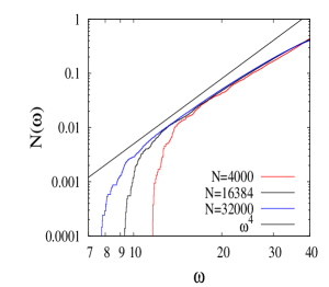
We check our experimental findings using Monte-Carlo simulation of a hard sphere crystal. We use a face-centered cubic crystal made of 864 particles, with periodic boundary conditions. We thermally equilibrate the system over a sufficient number ($10^{6}$) of MC steps. We compute the covariance matrix (Eq. 6) to find the eigenmodes of the system along runs of $10^{5}$ MC sweeps, out of which we use $5\times 10^{4}$ snapshots for time averaging. We obtain the matrix for both the whole three dimensional system and two dimensional $(111)$ planes, in order to mimic the experimental conditions (see also [14] for a comparison between the $3d$ simulations and a $2d$ cut). As the number of particles (and thus modes) in a two dimensional plane is quite small, we average over several planes. The density of states we obtain is shown in Fig. 5. For the low frequency part of the cumulative DOS of the two dimensional slice we again find a cumulative density of states which seems to converge to $N(\omega)\sim\omega^{4}$ when we increase the system size, which is compatible with the experimental data. Data with $N=32000$ can be fitted by exponents between $3.7$ and $4.1$.”

Figure 5: Left: Density of states for a two dimensional section of a 3D hard sphere crystal (with $N=4000$) from Monte-Carlo simulation. Right: Low frequency part of the cumulative DOS for two dimensional slices of the three dimensional system for three system sizes, with logarithmic scale, showing a powerlaw behavior compatible with the Debye behavior $N(\omega)\sim\omega^{4}$. Note that the range over which the scaling holds increases with the system size, indicating a convergence to the expected result. Frequencies are in unit of the inverse particle diameter.

We now turn to a simple scalar theory which gives an indication as to how Debye theory must be modified when one observes two dimensional cuts of a three dimensional sample.

The elastic energy of a three dimensional crystal can be written in terms of a symmetric shear tensor $u_{i,j}$ and three independent elastic constants. At large length scales correlations in displacement fluctuations decay as $1/r$, but are also characterized by a complicated tensorial structure coming from the cubic anisotropy of the crystal.

The effect of the large distance decay can be found in a much simpler theory based on a scalar field $u$ rather than the vector $u_{i}$. This scalar can be thought of as being, for instance, the amplitude of longitudinal fluctuation which couple to density fluctuations. The advantage of such a description is an enormous simplification in the tensorial algebra and a simple closed form for the projected correlation function. It is possible to perform a detailed tensorial calculation, which we will publish in the future and which yields very similar results.

We therefore consider fluctuations of a scalar quantity $u$ with an energy which is of the form

$$U=\frac{A}{2}\int(\nabla u)^{2}d^{3}\bf{r}$$ (7)

where $A$ is an elastic modulus. In the generalization to elastic fluctuations one would consider an energy based on the symmetrized strain tensor. In Fourier space the energy has the form

$$U=\frac{A}{2}\sum_{k}k^{2}|u_{k}^{2}|$$ (8)

we notice the usual scaling of the elastic energy in $k^{2}$.

In an underdamped system with kinetic energy $\rho\dot{u}^{2}/2$ this gives rise to the dispersion relation $\omega^{2}=c^{2}k^{2}$. One thus expects a density of states

$${\rm d}N\sim k^{2}\,{\rm d}k\sim\omega^{2}{\rm d}\omega$$ (9)

It is this scaling of the density of states in $\omega^{2}$ that is known from the theory of Debye.

In a three dimensional sample thermal fluctuations excite the system, so that equipartition and eq. (8) implies

$$\langle|u_{k}|^{2}\rangle=\frac{k_{B}T}{Ak^{2}}$$ (10)

This gives a decay of correlations in real space which is given by the inverse Fourier transform of $1/k^{2}$. We can find the result immediately by reference to electrostatics:

$$\langle u(i)u(j)\rangle=\frac{1}{4\pi A|r_{i}-r_{j}|}$$ (11)

a Coulomb like decay of correlations.

Now take a two dimensional slice of the system. Within this slice the correlations are still decaying as $1/r$. We wish to describe what we see, however, in terms of a purely two-dimensional theory, so we perform a two dimensional Fourier transform to find the effective stiffness. Thus

$$\langle|u_{k}|^{2}\rangle_{2}=\int\frac{1}{Ar}\,e^{i{k}_{2}\cdot{r}}\,d^{2}\,{r}\,=\frac{1}{2A|k_{2}|}$$ (12)

where we use the subscript $2$ to indicate that we are working with the two-dimensional projected objects. The result is rather interesting: rather than correlations in three dimensional being described by a decay in $1/k^{2}$ we find a slower decay: $1/|k_{2}|$.

Now that we have the scaling form of the correlations we can work backwards and deduce the effective elastic theory in two dimensions

$$U_{2}=\frac{A}{2}\sum_{k_{2}}2|k_{2}||u_{k_{2}}|_{2}^{2}$$ (13)

Thus the elastic behavior in real space corresponds to fractional derivatives of the field $u$ leading to long-ranged effective interactions in the projected system.

We now calculate the “propagative” eigenvalue by defining

$$\omega_{2}^{2}=2A|k_{2}|$$ (14)

which is the analogy of $\omega^{2}=c^{2}k^{2}$ that we use in three dimensions. We note that the dispersion law is very different from that of usual elastic problems. The density of states of this two dimensional matrix are just

$${\rm d}N_{2}\sim k_{2}{\rm d}k_{2}\sim\frac{\omega_{2}^{3}}{A^{2}}{\rm d}\omega_{2}$$ (15)

The density of states is thus $D(\omega)\sim\omega_{2}^{3}$ and the integrated density of the states $N(\omega)\sim\omega_{2}^{4}$, in good agreement with what was found in the experiment and in the simulations.

2.1 Comparision of methods

In this section we briefly discuss and compare the two methods adopted in the present study to obtain the spectrum namely the $2\times 2$ dynamical matrix $K_{\mu\nu}^{-1}(k)$ and the spatial covariance matrix described in Eq. 6. To establish a correspondence we compute the full $2N\times 2N$ matrix in k-space,

$$\tilde{Q}_{\mu\nu}(k,k^{\prime})=\langle u^{*}_{\mu}(k)u_{\nu}(k^{\prime})\rangle.$$ (16)

Figure 6: Normal mode spectrum: Cumulative Density of states and DOS for the present crystal as obtained from the covariance matrix $Q_{\mu\nu}(r_{i},r_{j})$ in real space and its equivalent $\bar{Q}(k,k^{\prime})$ in Fourier space. For a perfect crystal these two methods should give identical results. In the case of imperfections the modes $|k\rangle$ and $|k^{\prime}\rangle$ are no longer orthonormal leading to small differences in the spectra.

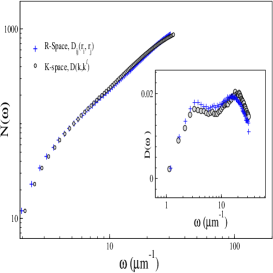
using the same Fourier components of displacements as described earlier (Eq. 2), which includes the non-orthogonal correlations as well. Let us first discuss the results obtained from the full diagonalization of both $\tilde{Q}$ matrices (Eqs. 6 and 16). Fig. 6 compares the spectrum - DOS and cumulative DOS for both the methods: they nearly coincide. This confirms the equivalence of the spatial matrix $Q_{\mu\nu}(i,j)$ with $\tilde{Q}_{\mu\nu}(k,k^{\prime})$ and supports the fact that the data are not affected by the choice of the boundary conditions or imperfections of the crystal. Now, the diagonal elements of $\tilde{Q}_{\mu\nu}(k,k^{\prime})$ correspond to $K_{\mu\nu}^{-1}$ but the non-diagonal elements in $(k,k^{\prime})$ encode information about the heterogeneity and imperfections of the sample. Thus, with negligible imperfections in the crystal and a sufficiently long averaging time, the spectrum from all three methods should coincide with each other.

2.2 Conclusions

We have studied the dynamics of a hard sphere colloidal crystal at a volume fraction $\phi\sim 0.57$, a volume fraction slightly above the melting transition, using confocal microscopy. The density of states and normal modes were obtained from measured particle displacements. Hard sphere systems are usually weakly connected and the interaction potential is strongly anharmonic; however the present observations shows that the lowest frequency modes are extended plane waves-like as can be expected for a harmonic solid. In addition we have shown that the density of states can be understood using continuum elasticity theory.

The effective exponent for the frequency-dependence of the density of states was measured in the low energy regime and is inconsistent with the expected Debye behavior in $D(\omega)\sim\omega^{d-1}$ for both $d=2$ and $d=3$. We found that the data can be explained by a theory with an unusual energy dispersion relation in $|k_{2}|$, which gives $D(\omega)\sim\omega^{3}$. This expression agrees with both the experiments and the simulations. It is interesting to note that the same energy function was found in [16] where the spreading of a droplet was expressed as the effective dynamics of a contact line. Again we are in the presence of a physical system projected to lower dimensions.

We appreciated discussions with Jorge Kurchan and Gerard Wegdam. The present project is supported by FOM.

References

- [1] P. N. Pusey & W. van Megen, Nature, 320, 1986, 340.
- [2] M. D. Rintoul & S. Torquato , Phys. Rev. Lett. 77, 1996, 4198.
- [3] D. J. W. Aastuen, N. A. Clark, K. L Cotter & J. B. Ackerson Phys. Rev. Lett. 57, 1986, 1733.
- [4] P.N. Pusey & W. van Megen Nature, 320, 1986, 340.
- [5] P. Keim, G. Maret, U. Herz & H. H von Grünberg Phys. Rev. Lett. 92, 2004, 21550.
- [6] K. Zahn, A. Wille, G. Maret, S. Sengupta & P. Nielaba Phys. Rev. Lett., 90, 2003, 155506.
- [7] E. B Sirota, H. Ou-Yang, S. K. Sinha., P. M. Chaikin , J. D. Axe & Y. Fujii, Phys. Rev. Lett., 62, 1989, 1524.
- [8] Z. Cheng, J. Zhu, W. B. Russel & P. M. Chaikin, Phys. Rev. Lett., 85, 2000,1460.
- [9] S. R. Penciu, M. Kafesaki, G. Fytas, E. N. Economou, W. Steffen A Hollingsworth & W. B Russel EPL (Europhysics Letters) 58, 2002, 699.
- [10] A. K. Ghatak & L. S. Kothari, An Introduction to Lattice Dynamics (Addison-Wesley, New York), 1972.
- [11] A. Ghosh, V. K. Chikkadi, P. Schall, J. Kurchan & D. Bonn Phys. Rev. Lett. 104, 2010, 248305.
- [12] D. Kaya, N. L. Green, C. E. Maloney & M. F. Islam, Science 329, 2010, 656.
- [13] K. Chen, W. G. Ellenbroek, Z. Zhang, D. T. N Chen, P. J. Yunker, S. Henkes C. Brito, O. Dauchot, W. van Saarloos, A. J. Liu & A. G. Yodh Phys. Rev. Lett. 105, 2010, 025501.
- [14] A. Ghosh, R. Mari , V. K. Chikkadi, P. Schall, J. Kurchan & Bonn D. Soft Matter, 6, 2010, 3082.
- [15] C. Brito, O. Dauchot, G. Biroli & J. P. Bouchaud , Soft Matter 6, 2010, 3013.
- [16] J. F. Joanny & P.G. de Gennes J. Chem. Phys. 81, 1984, 552.