The Swift Serendipitous Survey in deep XRT GRB fields (SwiftFT)
I. The X-ray catalog and number counts

Abstract

Aims. An accurate census of the active galactic nuclei (AGN) is a key step in investigating the nature of the correlation between the growth and evolution of super massive black holes and galaxy evolution. X-ray surveys provide one of the most efficient ways of selecting AGN.

Methods. We searched for X-ray serendipitous sources in over 370 Swift-XRT fields centered on gamma ray bursts detected between 2004 and 2008 and observed with total exposures ranging from 10 ks to over 1 Ms. This defines the Swift Serendipitous Survey in deep XRT GRB fields, which is quite broad compared to existing surveys ($\sim$33 square degrees) and medium depth, with a faintest flux limit of 7.2$\times 10^{-16}$ erg cm^-2 s^-1 in the 0.5 to 2 keV energy range (4.8$\times 10^{-15}$ erg cm^-2 s^-1 at 50% completeness). The survey has a high degree of uniformity thanks to the stable point spread function and small vignetting correction factors of the XRT, moreover is completely random on the sky as GRBs explode in totally unrelated parts of the sky.

Results. In this paper we present the sample and the X-ray number counts of the high Galactic-latitude sample, estimated with high statistics over a wide flux range (i.e., 7.2$\times 10^{-16}\div\sim 5\times 10^{-13}$ erg cm^-2 s^-1 in the 0.5-2 keV band and 3.4$\times 10^{-15}\div\sim 6\times 10^{-13}$ erg cm^-2 s^-1 in the 2-10 keV band). We detect 9387 point-like sources with a detection Poisson probability threshold of $\leq 2\times 10^{-5}$, in at least one of the three energy bands considered (i.e. 0.3-3 keV, 2-10 keV, and 0.3-10 keV), for the total sample, while 7071 point-like sources are found at high Galactic-latitudes (i.e. $\mid$b$\mid\geq$20 deg.). The large number of detected sources resulting from the combination of large area and deep flux limits make this survey a new important tool for investigating the evolution of AGN. In particular, the large area permits finding rare high-luminosity objects like QSO2, which are poorly sampled by other surveys, adding precious information for the luminosity function bright end. The high Galactic-latitude logN-logS relation is well determined over all the flux coverage, and it is nicely consistent with previous results at 1$\sigma$ confidence level. By the hard X-ray color analysis, we find that the Swift Serendipitous Survey in deep XRT GRB fields samples relatively unobscured and mildly obscured AGN, with a fraction of obscured sources of $\sim 37\%$ ($\sim 15\%$) in the 2-10 (0.3-3 keV) band.

1 Introduction

The “feedback” between the super-massive black holes (SMBH), which fuel the active galactic nuclei (AGN), and the star formation in the host galaxy tightly links the formation and evolution of AGN and galaxies. Therefore, a complete knowledge of the evolution and the phenomena in the AGN is a key topic in cosmology. A good way to complete the census of AGN is to use X-ray surveys, because these efficiently select AGN of many varieties at higher sky surface densities than at other wavelengths. The better capability of finding AGN in X-rays rests on three main causes: 1) X-rays directly trace accretion onto SMBH, providing a selection criterion that is less biased than the AGN optical emission line criterion; 2) AGN are the dominant population in the X-rays, because they are most ($\sim$ 80%) of the X-ray sources; 3) X-rays in the medium-hard band (i.e. $\sim$ 0.5-10 keV band, that is the energy coverage of Chandra and XMM-Newton) are able to detect unobscured and moderately obscured AGN (i.e. N_H${{}_{<}\atop{}^{\sim}}$ a few 10²³ cm^-2, Compton thin AGN).

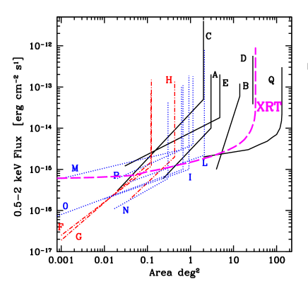
Chandra and XMM-Newton performed several deep pencil beam surveys and shallow wide contiguous surveys (see Fig. 1). Deep pencil beam surveys (see Table 1) are fundamental in studying the population of faintest X-ray sources, especially the emerging new population of “normal” galaxies (Brandt & Hasinger 2005); however, because they sample very small sky regions, they are strongly affected by cosmic variance. Wide shallow contiguous surveys (see Table 1) are complementary to deep pencil beam surveys, since they are less affected by cosmic variance, by covering a much larger area of the sky. Nevertheless they only reach relatively high fluxes, losing a large fraction of faint AGN.

The gap between deep pencil beam surveys and the wide contiguous shallow surveys is filled by the very large, non-contiguous, medium-depth surveys. This type of survey, based on the large archival data available from Chandra and XMM-Newton satellites (see Table 1), covers very large sky area, thus finding rare objects, like the highest luminosity, obscured AGN, QSO2 (see e.g. HELLAS2XMM, Fiore et al. 2003). An additional fundamental advantage of this type of survey is the ability to investigate field to field variations of the X-ray source density, which may trace filaments and voids in the underlying large-scale structure.

Table 1: Main properties of the most famous X-ray surveys ( see Fig. 1).

Labela	Name	Area	Flux limit	Bandb	Reference
		deg.2	erg cm -2 s-1	keV
Examples of deep pencil beam surveys
G	CDFS	$\sim$0.1	1.9$\times$10-17	0.5-2	Giacconi et al. 2001, Luo et al. 2008
F	CDFN	$\sim$0.1	2.5$\times$10-17	0.5-2	Brandt et al. 2001, Alexander et al. 2003
H	XMM-Newton Lockman Hole	$\sim$0.43	$\sim$ 1.9$\times$10-16	0.5-2	Worsley et al. 2004, Brunner et al. 2008
Examples of wide shallow contiguous surveys
N	E-CDF-S	$\sim$0.3	1.1$\times$10-16	0.5-2	Lehmer et al. 2005
M	ELAIS-S1	$\sim$0.6	5.5$\times$10-16	0.5-2	Puccetti et al. 2006
L	XMM-COSMOS	$\sim$2	1.7$\times$10-15	0.5-2	Hasinger et al. 2007, Cappelluti et al. 2007, 2009
I	C-COSMOS	$\sim$1	1.9$\times$10-16	0.5-2	Elvis et al. 2009
O	AEGIS-X	0.67	5$\times$10-17	0.5-2	Laird et al. 2009
Examples of surveys based on serendipitous sources in archival data
A	Hellas2XMM	3	5.9$\times$10-16	0.5-2	Baldi et al. 2002
C	SEXSI	$\sim$2	5$\times$10-16	2-10	Harrison et al. 2003
D	XMM-BSS	28.1	7$\times$10-14	0.5-4.5	Della Ceca et al. 2004
E	AXIS	4.8	$\sim$2$\times$10-15	2-10	Carrera et al. 2007
P	SXDS	1.14	6$\times$10-16	0.5-2	Ueda et al. 2008
B	CHAMP	$\sim$10	$\sim$10-15	0.5-2	Kim et al. 2007
Q	TwoXMM ($\mid$b$\mid$$\geq 20$)	$\sim$132.3	$\sim$2$\times$10-15	0.5-2	Mateos et al. 2008

^a Label refers to Fig. 1;

^b The flux limit is related to this energy band.

We built a new large medium-depth X-ray survey searching for serendipitous sources in images taken by the Swift (Gehrels et al. 2004) X-ray telescope XRT (Burrows et al. 2005) centered on gamma-ray bursts (GRBs). The Swift Serendipitous Survey in deep XRT GRB fields (SwiftFT) presents significant advantages compared with present large area X-ray surveys. First, Swift is a mission devoted to discovering GRBs and following their afterglows, which in X-rays last typically several days after the burst, so the same sky region can be observed for very long exposure (as long as $\sim$1.17 Ms in the case of GRB060729). This, together with the very low and stable background of the XRT camera ($\sim$0.0002 counts sec^-1 arcmin^-2 in the 0.3-3 keV band) permits us to have flux limit of $\sim$7.2$\times$10^-16 erg cm^-2s^-1 in the 0.5-2 keV (50% completeness flux limit of 4.8$\times 10^{-15}$ erg cm^-2 s^-1, for conversion from rate to flux see Sec. 4.3), one of the deepest flux limits of any large area survey. Second, the XRT point spread function and vignetting factor, being approximately independent of the distance from the aim point of the observation (i.e. off-axis angle), secure a uniform sky coverage. This uniform sensitivity provides the largest area coverage at the lowest flux limits (see Fig. 1). Third, since GRBs explode randomly on the sky, with an isotropic distribution (Briggs et al. 1996), the SwiftFT does not suffer any bias toward previously known bright X-ray sources, as the large serendipitous surveys based on X-ray archival data, like Einstein, ROSAT, Chandra and XMM-Newton data (see also Moretti et al. 2009). Specifically, a correlation length of 1-10 Mpc corresponds to $\sim$2-20 arcmin at the mean redshift of the Swift GRBs (i.e. z$=2.1\pm 1.5$, in a cosmological model ($\Omega_{M}$, $\Omega_{\lambda}$)=(0.3,0.7)) and to $\sim$10-100 arcmin at the typical redshift of known X-ray targets (i.e. z$\leq$0.1). This implies that in the case of GRBs, the detection of serendipitous sources, that might be associated with large scale structure around the target, is less probable (see e.g. D’Elia et al. 2004 and references therein).

In this paper we report on the strategy, design and execution of the SwiftFT: in Sect. 2 we give an overview of the survey and briefly present the analyzed observations, in Sec. 3 and 4 we describe the data reduction, detection method and source characterization procedure, respectively. In Sect. 5 we show the catalog of the point-like X-ray sources. For the high Galactic-latitude fields (i.e. $\mid$b$\mid$$\geq$20 deg), we present the survey sensitivity, the X-ray number counts (i.e. LogN-LogS) and the hardness ratio analysis in Sec. 6. Finally Sec. 7 shows our conclusion.

Figure 1: The flux limit in the 0.5-2 keV band vs. the area coverage for various surveys. Magenta long dashed lines are the total XRT Deep Serendipitous Survey; black solid lines are medium large not contiguous surveys: A: H2XMM, B: CHAMP, C: SEXSI, D: XMM-BBS, E: AXIS , Q: twoXMM ($|$b$|>$20); red dot short-dashed lines are the smallest and very deep surveys: F: CDFN, G: CDFS, H: LockmanHole; blue dotted lines are shallow contiguous survey I: CCOSMOS, L: XMMCOSMOS, M: ELAIS-S1, N: ECDFS, O: AEGISX, P: SXDS (for references see Table 1).

2 The Swift Serendipitous Survey in deep XRT GRB fields

The Swift mission (Gerhels et al. 2004) is a multi-wavelength observatory dedicated to GRB astronomy. Swift’s Burst Alert Telescope (BAT) searches the sky for new GRBs, and, upon discovering one, triggers an autonomous spacecraft slew to bring the burst into the X-ray Telescope (XRT) and Ultraviolet/Optical Telescope (UVOT) fields of view. XRT and UVOT follow the GRB afterglow while it remains detectable, usually for several days. This is achieved by performing several separate observations of each GRB. By stacking individual exposures it is possible to build a large sample of deep X-ray images. To this purpose, we considered all GRBs observed by Swift from January 2005 to December 2008, with a total exposure time in the XRT longer than 10 ks. We also analyzed the XRT 0.5 Ms observations of the Chandra Deep Field-South (CDFS) sky region. 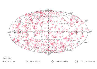We call this set of observations the Swift Serendipitous Survey in deep XRT GRB fields (SwiftFT). As GRBs explode at random positions in the sky the pointing positions of the 374 fields selected in this way are completely random as shown in Fig. 2. 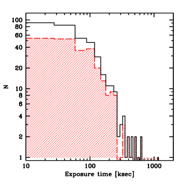The total exposure time is 36.8 Ms, with $\sim$32% of the fields having more than 100 ks exposure time, and $\sim$28% with exposure time in the range 50-100 ks (see top panel of Fig. 3). The SwiftFT covers a total area of $\sim$32.55 square degrees; the bottom panel of Fig. 3 shows the exposure time versus the survey area. A complete list of the fields is available on-line at this address http://www.asdc.asi.it/xrtgrbdeep_cat/logXRTFIELDS.pdf. This table for each field gives the field name, the R.A., the Dec., the start-DATE, the end-DATE and the total exposure time.
In this paper we concentrate on extragalactic X-ray sources so we consider in detail the 254 fields at high Galactic-latitudes ($\mid$b$\mid\geq$20, HGL catalog hereinafter), which cover a total area of $\sim$22.15 square degrees and have a total exposure time of 27.62 Ms (see Fig. 2 and 3).

Figure 2: Aitoff Projection in Galactic coordinates of the 374 SWIFT-XRT fields analyzed so far. The dot sizes are proportional to the total field exposure time.

Figure 3: Top panel: the distribution of the field’s exposure times in ks, for the total sample (black solid histogram) and the HGL sample (red dashed histogram).Bottom panel: the survey areas vs the effective exposure time.

3 XRT data reduction

The XRT data were processed using the XRTDAS software (Capalbi et al. 2005) developed at the ASI Science Data Center and included in the HEAsoft 6.4 package distributed by HEASARC. For each field of the sample, calibrated and cleaned Photon Counting (PC) mode event files were produced with the xrtpipeline task. In addition to the screening criteria used by the standard pipeline processing, a further, more restrictive, screening was applied to the data, in order to improve the signal to noise ratio of the faintest, background dominated, serendipitous sources.

Therefore we selected only time intervals with CCD temperature less than $-50$ $\deg$C (instead of the standard limit of $-47$ $\deg$C) since the contamination by dark current and hot pixels, which increase the low energy background, is strongly temperature dependent. Moreover, to exclude the background due to residual bright earth contamination, we monitored the count rate in four regions of 70$\times$350 physical pixels, located along the four sides of the CCD. Then, through the xselect package, we excluded time intervals when the count rate was greater than 40 counts/s. This procedure allowed us to eliminate background spikes, due to scattered optical light, that usually occur towards the end of each orbit when the angle between the pointing direction of the satellite and the day-night terminator (i.e. bright earth angle, BR_EARTH) is low.

We performed the on-ground time dependent bias adjustment choosing, in each time interval, a single bias value using the entire CCD window and we applied this value to all the events collected during the time interval. Finally we note that multiple observations of the same field may differ somewhat in aim point and roll angle. In order to have a uniform exposure, we restricted our analysis to a circular area of 10 arcmin radius, centered in the median of the individual aim points. The observations of each field were processed providing an input to the xrtpipeline of a fixed pointing direction chosen as the median of the different pointings on the same target. The cleaned event files obtained with this procedure were merged using xselect. In some of the deepest images of our sample ($>200$ ks) we found evidence of several hot pixels along the detector column DETX$=$295; therefore we excluded this column from our analysis.

As for the event files, we produced exposure maps of the individual observations, providing as input to the xrtexpomap a fixed pointing direction equal to the median of the pointings on the same target. The corresponding total exposure maps were generated by summing the exposure maps of the individual observations with XIMAGE. We produced exposure maps at three energies: 1.0 keV, 4.5 keV, and 1.5 keV. These correspond to the mean values for a power-law spectrum of photon index $\Gamma$$=1.8$ (see Sec 4.3) weighted by the XRT efficiency over the three energy ranges: 0.3-3 keV (soft band S), 2-10 keV (hard band H), 0.3-10 keV (full band F) considered.
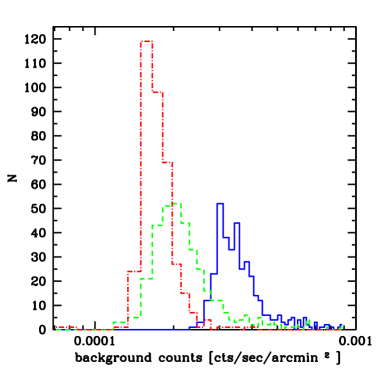
For each field we also produced a background map, using XIMAGE by eliminating the detected sources and calculating the mean background in box cells of size 32$\times$32 pixels. Fig. 4 shows the distribution of the mean background counts/s/arcmin² in the three energy bands: S, H and F. The median values of background and their interquartile range are 0.22$\pm$0.04 counts/ks/arcmin², 0.17$\pm$0.01 counts/ks/arcmin² and 0.35$\pm$0.05 counts/ks/arcmin² for the S, H and F band, respectively. These median values correspond to a level of less than 1 count in the S, H, and F band, over a typical source detection cell (see Sec. 4.1) and exposure of 100 ks. The low background is important for the detection of the faintest sources.

Figure 4: The distribution of the mean background counts/sec/arcmin² for the 374 XRT fields, in the F band (blue solid histogram), S band (green dashed histogram), and H band (red dot-dashed histogram).

4 Data analysis

4.1 Source Detection

The X-ray point source catalog was produced by the detection algorithm detect, a tool of the XIMAGE PACKAGE version 4.4.1 . Detect locates the point sources using a sliding-cell method. The average background intensity is estimated in several small square boxes uniformly located within the image. The position and intensity of each detected source are calculated in a box whose size maximizes the signal-to-noise ratio. The net counts are corrected for dead times and vignetting using the input exposure maps, and for the fraction of source counts that fall outside the box where the net counts are estimated, using the PSF calibration. Count rate statistical and systematic uncertainties, are added quadratically. We set detect to work in bright mode, that is recommended for crowded fields and fields containing bright sources, since it does not merge the excess before optimizing the box centroid (see the XIMAGE help). We tested detect on a sample of fields, with deep and medium deep exposure times, to determine the other detection parameters, that are the most suitable for our survey. To this end we also compared the results of detect applied to the field GRB070125, with the results of the ewave detection algorithm of CIAO applied to the Chandra observations of the same field. We found that background is well evaluated for all exposure times, using a box size of 32$\times$32 original detector pixels, and that the optimized size of the search cell, that minimizes source confusion, is 4$\times$4 original detector pixels. We also set the signal-to-noise acceptance threshold to 2.5. We produced a catalog using a Poisson probability threshold of 4$\times 10^{-4}$. Here we present only a more conservative catalog cut to a probability threshold of 2$\times 10^{-5}$, to minimize the number of spurious sources. This probability corresponds to about 0.24 spurious sources for each field (see Sec. 4.2)
We applied detect on the XRT image using the original pixel size, and in the three energy bands: F, S and H (see Sec. 3). For each field we detected only sources in a circular area of 10 arcmin radius centered in the median of the individual aim points (see Sect. 3). We find that a straight application of detect on those images to which the spatial filter was applied leads to an incorrect estimate of the count rates from the sources near the edges of the circular area; this is a consequence of the inaccurate PSF correction and a poorly estimated background at the image edges. To overcome this difficulty, we applied a two step spatial filter. We first ran detect on the images to which the spatial filter was applied, to select only a circular area of 10.5 arcmin radius centered at the median of the individual aim points. Then, we applied a second spatial filter to the catalog, accepting only sources whose distance from the image center is equal to, or less than, 10 arcmin.
This catalog was cleaned from obvious spurious sources, like detection on the wings of the PSF or near the edges of the XRT CCD, spurious fluctuations on extended sources etc., through visual inspection of the XRT images in the three energy bands. We eliminated the GRBs by matching the catalog with the GRB positions by Evans et al. 2009. Moreover we also eliminated extended sources from the final point-like catalog, because detect is not optimized to detect this type of sources, not being calibrated to correct for the background and PSF loss in case of extended sources (a detailed catalog of the extended sources will be presented in a forthcoming paper by Moretti et al.). We built a list of candidate of extended sources, by checking for each candidate source if detect finds a clusters of spurious sources on the diffuse emission, and/or if the X-ray contours show extended emission. Then, we verified that a source is actually extended, by comparing the source brightness profile with the XRT PSF at the source position on the detector, using XIMAGE. We find that the number of these clearly extended sources is $<10\%$ and $<9\%$ of the sample, at a detection significance level of P$=$4$\times 10^{-4}$ and P$=$2$\times 10^{-5}$, respectively. Finally we refined the source position by the task xrtcentroid of the XRTDAS package.

4.2 Catalog reliability

To evaluate the number of spurious sources corresponding to the chosen probability threshold of 2$\times 10^{-5}$, we simulated 45 XRT fields, with the same characteristics (i.e. number of observations, exposure times, R.A. and Dec. of the single pointings) of the fields, which were randomly chosen among the 374 XRT fields.

The simulations were made up by an X-ray event simulator, developed at the ASI Science Data Center (ASDC), already used for missions like Beppo-SAX, Simbol-X, Nustar, Swift-XRT (see e.g. the flow chart in Puccetti et al. 2009b, and a few examples of applications in Puccetti et al. 2008, Fiore et al. 2008, 2009.). For Swift-XRT we updated the ASDC simulator with the calibration files distributed by heasarc (i.e. the vignetting function, the analytical function describing the PSF and the response matrix files) and with the XRT background described in Moretti et al. 2009. The simulated sources is randomly drawn from the 0.5-2 keV X-ray number counts predicted by the AGN population synthesis model by Gilli et al. (2007).

For each field we first simulated an observation with an exposure time increased by a factor of 5 compared to the original value, to generate a source list deeper than that of the original XRT field. This source list was then used as input for each of the observations of the same XRT field. Finally we summed all the observations of the same field, as for the real fields (see Sec. 3) and applied the detector procedure and the visual cleaning described in Sec. 4.1. We matched the input and the detected source lists using a maximum likelihood algorithm with maximum distance of 6 arcs, to find the most probable association between an input source and an output detected source. By this analysis, we find a total of 11 spurious sources in the 45 simulated fields. Therefore we evaluated an average number of spurious sources of 0.24 for each field in the three energy bands (S, H, and F) at the probability threshold of 2$\times 10^{-5}$.

4.3 Count rates, fluxes

For a sample of 20 sources in a broad range of brightness (F flux in the range 3.9$\times$10^-15$\div$1.3$\times$10^-14 erg cm^-2 s^-1) and off-axis angles, we compared the count rates evaluated using the detect algorithm with the count rates measured from the spectra extracted using a radius of 20 arcs, which corresponds to a f_psf$\sim$70%-80%, depending on energy and off-axis angle. The count rates measured from the spectra were then corrected for the f_psf and the telescope vignetting, using the appropriate response matrix. The average ratio between the count rates given by the detect algorithm and those measured from the spectra is 1.1$\pm$0.2, indicating a good consistency between the two methods at 1$\sigma$ confidence level.
For the high Galactic-latitude sample ($\mid$b$\mid\geq$20, HGL catalog hereinafter), in order to be consistent with other results present in the literature, count rates estimated in the S, H and F band were extrapolated to 0.5–2 keV, 2–10 keV and 0.5–10 keV fluxes, respectively. To convert count rates into fluxes, we assumed that the typical spectrum of the HGL sources is a simple power-law model absorbed by the Galactic column density along the line of sight. We chose to fix N_H to the median of the Galactic N_H of the HGL fields, that is 3.3$\times 10^{20}$ cm^-2 with an interquartile range of 1.4$\times 10^{20}$ cm^-2(see Fig. 5). We then fixed the spectral slope of the power-law model, to the most probable value, according to the distribution of the hardness ratio, defined as HR=(c_H-c_S)/($c_{H}$+c_S), where c_S and c_H are the S and H count rates of the HGL sources detected in both the bands, respectively. Following Mateos et al. (2008), we assume that each source has an HR distributed as a Gaussian with mean value HR and $\sigma$, the 68% error on HR. We then calculated the integrated probability by adding the probability density distributions of the HR of each source (see Fig. 6). We find that the most probable value is HR$\simeq$-0.5, that for N_H=3.3$\times 10^{20}$ cm^-2, corresponds to a photon spectral index $\Gamma$=1.8, assuming a power law model.

Count rates were converted to fluxes using the conversion factors quoted in the first line of Table 2, which are appropriate for a power law spectrum with photon spectral index $\Gamma$=1.8, absorbed by a Galactic N_H$=$3.3$\times 10^{20}$ cm^-2. The major uncertainty in the estimate of the fluxes is due to the variety of intrinsic spectra of the X-ray sources. Moreover the average spectral properties are a function of the observed flux (Brandt & Hasinger 2005). To estimate this uncertainty, we calculated the count rates to fluxes conversion factors for power law spectra with $\Gamma=$1.4, and for absorbed power law spectra with $\Gamma=$1.4 and 1.8, and N${}_{H}=10^{22}$ cm^-2. The conversion factors are in ranges of $\sim$1-1.3,$\sim$1.1-1.2 and $\sim$1.3-2.1, in the S, H and F band, respectively (see Table 2). The conversion factor for the F band is more sensitive to the spectral shape than for the S and H bands, because it is wider.

For the low Galactic-latitude sources we used the same conversion factors of the HGL sample, to convert count rates to fluxes.

Figure 5: Distribution of the Galactic hydrogen column density for the 254 HGL fields. The dotted line indicates the median value 3.3$\times$10²⁰cm^-2.

Figure 6: Relative probability density distribution of the hardness ratio (H-S)/(H+S) for the high Galactic-latitude sample. The dashed line indicates the most probable value of hardness ratio, which corresponds to a power-law spectral model with $\Gamma=1.8$, absorbed by an hydrogen column density N_H$=$3.3$\times 10^{20}$ cm^-2.

Table 2: Count rate to flux conversion factors for different spectral models.

$\Gamma$	NH	CF(F)a	CF(S)b	CF(H)c
	$10^{22}$ cm-2	cts s-1 $/$10-11 erg cm-2 s-1	cts s-1 $/$10-11 erg cm-2 s-1	cts s-1 $/$10-11 erg cm-2 s-1
1.8	0.033	3.641	1.591	8.090
1.4	0.033	4.868	1.565	9.283
1.4	1	7.720	1.232	9.880
1.8	1	6.324	1.326	8.620

^aenergy conversion factor to convert the F band count rate into 0.5-10 keV flux assuming an absorbed power-law spectrum with hydrogen column density N_H and photon index $\Gamma$;

^bsame as ^a, but to convert the S band count rate into the 0.5-2 keV flux;

^csame as ^a, but to convert the H band count rate into the 2-10 keV flux.

4.4 Upper limits

If a source is not detected in one band, we give a 90% upper limits to the source count rates and fluxes. The upper limits are computed following Puccetti et al. 2009. If M is the number of counts measured at the position of each source in a region of 16.5 arcs radius, which corresponds to a mean f_psf of $\sim 68\%$, B are the background counts, evaluated by the background maps (see Sec. 3), and $\sigma=$$\sqrt{B}$, the 90% upper limit is defined as the number of counts X that gives 10% probability to observe M (or less) counts equal to the Poisson probability:

$$P_{Poisson}=e^{-(X+B)}\sum_{i=0}^{M}{(X+B)^{i}\over i!}$$ (1)

We solved Eq. 1 iteratively for a 10% probability. The X upper limits derived with Eq. 1 do not take into account the statistical fluctuations on the expected number of background counts. In order to take the background fluctuations into consideration, we used the following procedure: if $\sigma(B)$ is the root mean square of B (e.g., $\sigma(B)=\sqrt{(}B)$ for large B), we estimated the 90% lower limit on B as B(90%)$=$B-1.282$\times\sigma$(B) and, as a consequence, the “correct” 90% upper limit (Y) becomes $Y=X\times 1.282\times\sigma$.

Vignetting corrected count rates limits for each source are obtained by dividing the count upper limits by the net exposure time, reduced by the vignetting at the position of each source, as in the corresponding exposure maps (see Sec. 3) and by correcting for the f_psf.

4.5 Positional error

The total positional uncertainty results from the combination of the statistical uncertainty (i.e. $\sigma_{stat}$), that depends on the instrumental PSF at the position of the source and is inversely proportional to the source counts, and of the uncertainty on the XRT aspect solution (i.e. $\sigma_{asp}$). The total positional uncertainty is:

$$err_{pos}=\sqrt{{\sigma_{stat}}^{2}+{\sigma_{asp}}^{2}}$$ (2)

We evaluated the positional errors at 68% and 90%. The $\sigma_{stat}$ at 68% level confidence are evaluated by dividing the PSF_radius corresponding to a mean f_psf of 68% (i.e $\sim$16.5 arcs) to the square root of the background subtracted source counts from aperture photometry, following Puccetti et al. (2009).
The aperture photometry values are derived from the total event data for each field. To extract source counts, circular regions centered on each source with a 16.5 arcs radius, corresponding to a mean f_psf of 68% for different off-axis angles and energies, are used. The background counts are extracted from the background maps calculated as described in Sec. 3.
The $\sigma_{stat}$ at 90% level confidence are evaluated following the formula by Hill et al. (2004): R$\times$counts^-0.48, with R$=$22.6 arcs and counts are the background subtracted source counts corresponding to a mean f_psf of $\sim$80%.

We cross-correlated the XRT catalog cut at a significance level of P$=$2$\times$10^-5 and with source count rate equal or greater than 0.001 ct/s, with the SDSS optical galaxy catalog to find the mean $\sigma_{asp}$ at 68% and 90% confidence level. For the cross-correlation, we used a match radius of 10 arcs, and a source positional uncertainty of $\sqrt{{\sigma_{stat68\%}}^{2}+{\sigma_{asp68\%}}^{2}}$ and $\sqrt{{\sigma_{stat90\%}}^{2}+{\sigma_{asp90\%}^{2}}}$, varying $\sigma_{asp68\%}$ and $\sigma_{asp90\%}$ to obtain that the XRT sources with an optical counterpart are 68% and 90%, respectively. In this way we find that the mean $\sigma_{asp}$ at 68% and 90% are 2.05 arcs and 3.55 arcs, respectively. The values of $\sigma_{asp}$ are consistent with previous results by Moretti et al. (2006).

The left panel of Fig. 7 shows the 68% positional errors as a function of the F band count rates, the solid line indicates the case in which the positional errors are exclusively due to $\sigma_{asp}$. The right panel of Fig. 7 shows the ratio between the 90% positional error and the 68% positional error vs. the F band count rates, the solid line is the case in which $\sigma_{stat}$ is equal to zero. We note that the positional error ratio is not Gaussian (i.e. equal to $\sim$1.65), probably due to the XRT PSF shape, which is not Gaussian.

Figure 7: Left panel: the 68% positional errors vs. the F band count rates, the solid line indicates the case with null statistical uncertainty ($\sigma_{stat}=0$). Right panel: ratio between the 90% positional error and the 68% positional error vs. the F band count rates, the solid line indicates the case with null statistical uncertainty ($\sigma_{stat}=0$)

.

4.6 Source confusion

In order to estimate the effects of source confusion on the HGL sample, we evaluated the probability P of finding two sources with flux F_x equal or higher than a flux threshold (F_xmin) at a distance closer than the minimum angular separation $\theta_{min}$, following:

$$P(<\theta_{min})=1-e^{-\pi N\theta^{2}_{min}}$$ (3)

where $\theta_{min}$ is set to twice the typical size of the source cell detection (i.e. 4 original pixel), and N is the number counts at F_xmin, evaluated by the X-ray number counts of C-COSMOS (Elvis et al. 2009).

The probability of finding two sources with flux higher than F_xmin= 2$\times 10^{-15}$ erg cm^-2 s^-1 and F_xmin= 1.1$\times 10^{-14}$ erg cm^-2 s^-1, for the S, and H bands, corresponding to a sky coverage of $\sim$2.2 square degrees (i.e. 10% of the HGL sky coverage), is only 4.6% and 2.3% for the S and H bands, respectively. These probabilities increase to 9% and 7.6% for fluxes corresponding to the faintest detected sources in the two bands.

4.7 CDFS: Swift-XRT vs Chandra

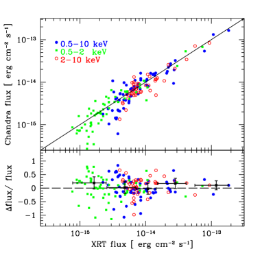
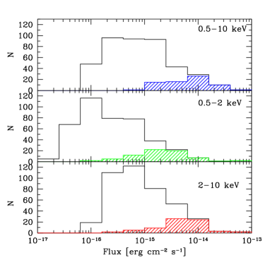
We applied the data cleaning, the source detection and source characterization described above, to the CDFS XRT data and compared the resulting CDFS XRT catalog, cut to a significance level of 2$\times 10^{-5}$ (see Sec. 4.2), to the Chandra catalog (Luo et al. 2008). We found that 71 out of 72 XRT sources are within the Chandra field. We matched the two CDFS catalogs using for each source either the error circle given by the sum of the squares of the XRT positional error (i.e. $\sigma_{XRT}(68\%)$ and $\sigma_{XRT}(90\%)$ at 68% and 90% level confidence, respectively) and Chandra 85% level confidence positional error (i.e. $\sigma_{Chandra}$) or a fixed distance conservatively of 10 arcs. Fig. 8 shows the ratio between the distance of the nearest Chandra source to each XRT source and the maximum radius $\sqrt{{\sigma_{XRT}(68\%)}^{2}+{\sigma_{\it Chandra}}^{2}}$ as well as the maximum radius $\sqrt{{\sigma_{XRT}(90\%)}^{2}+{\sigma_{\it Chandra}}^{2}}$ as a function of the count rates in the F band, if the source is detected in the F band, otherwise in the S band, otherwise in the H band. We find that the $\sim$80.2% and the $\sim$95.8% of the XRT CDFS sources have a Chandra counterpart, using the 68% and 90% level confidence XRT positional errors, respectively. Three XRT sources have a marginal Chandra detection at distance less than 6.5 arcs. Five XRT sources have two Chandra counterparts inside the error circle, which corresponds to $\sim$7% source confusion at a flux limit of $\sim$1.2$\times 10^{-15}$ and $\sim$4$\times 10^{-15}$ erg cm^-2 s^-1 in the S and H band, respectively. This percentage of source confusion is fully consistent with the estimate in Sec. 4.6. We then compared the XRT and Chandra fluxes in all the three bands 0.5-10 keV, 2-10 keV and 0.5-2 keV. We find good flux consistency (see left panel of Fig. 9), regardless of source variability. Actually the faintest XRT fluxes, near the flux limit, and the XRT fluxes around 3$\times 10^{-14}$ erg cm^-2 s^-1, although consistent at 1$\sigma$ confidence level with the Chandra fluxes, appear systematically greater than the Chandra fluxes (see left bottom panel of Fig. 9). This trend for the faintest XRT sources is probably due to the Eddington bias, while for the brightest sources the statistics are too poor to permit a firm comparison. Finally the right panel of Fig. 9 shows the comparison between the flux distribution of the total Chandra catalog and the Chandra source with XRT counterparts.

Figure 8: Ratio between the distance of the nearest Chandra source to each XRT source and the maximum radius $\sqrt{{\sigma_{XRT}(68\%)}^{2}+{\sigma_{\it Chandra}}^{2}}$ (open dots) as well as $\sqrt{{\sigma_{XRT}(90\%)}^{2}+{\sigma_{\it Chandra}}^{2}}$ (solid dots) as a function of the count rates in the F or S or H band (see Sec. 4.7).

Figure 9: Left top panel: the CDFS Chandra source fluxes vs. the XRT counterpart fluxes in the three energy band: 0.5-10 keV (blue solid dots), 2-10 keV (red open dots) and 0.5-2 keV (green solid squares). The solid line is the exact match between the Chandra and XRT fluxes. Left bottom panel: ratio between the relative difference of the XRT and Chandra fluxes vs. the XRT fluxes. The dashed line indicates the exact match between the Chandra and XRT fluxes, the stars are the mean ratios in each flux bin, with 1$\sigma$ uncertainties. Right panel: the empty histogram represents the flux distribution of the Chandra sources and the shaded histogram represents the flux distribution of the Chandra sources with an XRT counterpart, in the three energy band: 0.5-10 keV, 0.5-2 keV, 2-10 keV.

5 The point-source catalog

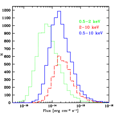
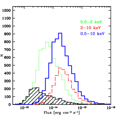
The detect tool was run on the three bands S, H and F. Table 3 gives the numbers of sources detected in each band with different significance level in both total and HGL catalog. We produced a unique catalog merging the individual S, H and F lists, using a matching radius of 6 arcs. We retained reliable sources, i.e. those with a significance level of being spurious $\leq$2$\times$10^-5 in at least one band, to limit the number of spurious detections to $\sim$0.24 for field. The final total and HGL catalog contain 9387 and 7071 sources, respectively. Table 4 reports the numbers of total and HGL catalog sources detected in three bands, two bands, or in only one band. Fig. 10 shows the flux distributions of the total sample (left panel) and of the HGL sample (right panel). We detect sources in the 0.5-2 keV and 2-10 keV bands down to flux limits of $\sim 7\times 10^{-16}$ ${\rm erg\leavevmode\nobreak\ cm}^{-2}\leavevmode\nobreak\ {\rm s}^{-1}$ and $\sim 4\times 10^{-15}$ ${\rm erg\leavevmode\nobreak\ cm}^{-2}\leavevmode\nobreak\ {\rm s}^{-1}$ , respectively. In comparison with a typical deep contiguous medium area survey, like C-COSMOS (Elvis et al. 2009, see Fig.10) the advantage of the SwiftFT is the definitely larger number of sources and the wider flux coverage, despite a slightly higher flux limit.

Figure 10: Left panel: the flux distributions of those sources detected in the S (green dotted histogram), H (red dashed histogram) and F (blue solid histogram) band in the total sample. Right panel: the flux distribution of those sources detected in the S (green dotted histogram), H (red dashed histogram) and F (blue solid histogram) band in the HGL sub-sample. The black shaded histogram represents the flux distribution of the 0.5-7 keV C-COSMOS sources (Elvis et al. 2009).

Table 3: Number of sources detected in each band at the two adopted probability thresholds.

Band	Na	N1b	NHGLc	NHGL1d
F	8719	880	6596	639
S	7925	684	6062	501
H	3791	436	2819	337

^a number of detected sources with detection significance level $\leq$ 2$\times 10^{-5}$;

^bnumber of detected sources with detection significance level: 2$\times 10^{-5}\leq$prob$\leq 4\times 10^{-4}$;

^c number of detected sources in the HGL fields, with detection significance level $\leq$2$\times 10^{-5}$;

^d number of detected sources in the HGL fields, with detection significance level: 2$\times 10^{-5}\leq$prob$\leq 4\times 10^{-4}$.

Table 4: Number of detected sources in the total SwiftFT catalog, with sources having a detection significance level $\leq$2$\times$10^-5 in at least one band.

Band	Na	NHGLb
F	8986	6797
S	8202	6253
H	4120	3088
F+S+H	3498	2671
F+S	4404	3371
F+H	521	354
F only	563	401
S only	300	211
H only	101	63

^a number of detected sources in the total SwiftFT catalog;

^b number of detected sources in the HGL catalog.

5.1 Catalog description

The full catalog is available on-line at this address http://www.asdc.asi.it/xrtgrbdeep_cat/. Table 5 gives the parameter descriptions of each source and Table 6 gives ten entries as an example.

Table 5: Source parameters in the catalog.

Column	Parameter	Description
1	NAME	source name: prefix SWIFTFTJ, following the standard IAU convention
2	RA	Swift-XRT Right Ascension in hms in the J2000 coordinate system.
3	DEC	Swift-XRT Declination in hms in the J2000 coordinate system.
4	pos_err	Positional error at 68% confidence level in arcs
5	pos_err	Positional error at 90% confidence level in arcs
6	X	X pixel coordinate
7	Y	Y pixel coordinate
8	Target name	XRT field
9	START-DATE	Start time of the field observations in year-month-day h:m:s
10	END-DATE	End time of the field observations in year-month-day h:m:s
11	ON-TIME	Total on-time in sec
12	f_rate	0.3–10 keV count rate or 90% upper limit in counts/sec
13	f_rate_err	1$\sigma$ 0.3–10 keV count rate error in counts/sec, in case of upper limits is set to -99
14	f_flux	0.5–10 keV Flux or 90% in erg cm-2s-1
15	f_flux_err	1$\sigma$ 0.5–10 keV Flux error in erg cm-2s-1, in case of upper limits is set to -99
16	f_prob	0.3–10 keV detection probability
17	f_snr	0.3–10 keV S/N
18	f_exptime	1.5 keV exposure time in ks from the exposure maps
19	s_rate	0.3–3 keV count rate or 90% upper limit in counts/sec
20	s_rate_err	1$\sigma$ 0.3–3 keV count rate error counts/sec, in case of upper limits is set to -99
21	s_flux	0.5–2 keV Flux or 90% upper limit in erg cm-2s-1
22	s_flux_err	1$\sigma$ 0.5–2 keV Flux error in erg cm-2s-1, in case of upper limits is set to -99
23	s_prob	0.3–13 keV detection probability
24	s_snr	0.3–3 keV S/N
25	s_exptime	1 keV exposure time in ks from the exposure maps
26	h_rate	2–10 keV count rate or 90% upper limit in counts/sec
27	h_rate_err	1$\sigma$ 2–10 keV count rate in counts/sec, in case of upper limits is set to -99
28	h_flux	2–10 keV Flux or 90% upper limit in erg cm-2s-1
29	h_flux_err	1$\sigma$ 2–10 keV Flux error in erg cm-2s-1, in case of upper limits is set to -99
31	h_snr	2–10 keV detection probability
30	h_prob	2–10 keV S/N
32	h_exptime	4.5 keV exposure time in ks from the exposure maps
33	hr	hardness ratio = (h_rate-s_rate)/ (h_rate+ s_rate)/
34	ehr	1$\sigma$ hardness ratio error evaluated with the error propagation formula (see e.g. Bevington 1992)
35	off-axis	distance from the field median center in arcmin
36	NH	Galactic hydrogen column density in cm-2

Table 6: Catalog template

NAME	RA	DEC	pos_err68	pos_err90	X	Y	Target name	START-DATE	END-DATE	ON-TIME
SWIFTFTJ000234-5301.1	00 02 34.6	-53 01 10.2	2.31	3.9	747.4	430.4	GRB070110	2007-01-10 07:27:08	2007-02-05 23:59:58	330057
SWIFTFTJ000238-5255.9	00 02 38.0	-52 55 54.1	2.55	4.1	734.5	564.5	GRB070110	2007-01-10 07:27:08	2007-02-05 23:59:58	330057
SWIFTFTJ000239-5301.6	00 02 39.1	-53 01 39.6	2.68	4.3	730.2	417.9	GRB070110	2007-01-10 07:27:08	2007-02-05 23:59:58	330057
SWIFTFTJ000243-5259.3	00 02 43.3	-52 59 22.9	3.93	5.8	713.9	476	GRB070110	2007-01-10 07:27:08	2007-02-05 23:59:58	330057
SWIFTFTJ000252-5259.5	00 02 52.8	-52 59 30.6	3.47	5.2	677.9	472.8	GRB070110	2007-01-10 07:27:08	2007-02-05 23:59:58	330057
SWIFTFTJ000254-5250.9	00 02 54.7	-52 50 54.4	4.28	6.2	670.9	691.8	GRB070110	2007-01-10 07:27:08	2007-02-05 23:59:58	330057
SWIFTFTJ000255-5253.8	00 02 55.3	-52 53 51.7	3.05	4.7	668.4	616.6	GRB070110	2007-01-10 07:27:08	2007-02-05 23:59:58	330057
SWIFTFTJ000258-5301.3	00 02 58.0	-53 01 19.1	3.56	5.3	657.9	426.8	GRB070110	2007-01-10 07:27:08	2007-02-05 23:59:58	330057
SWIFTFTJ000300-5259.9	00 03 00.9	-52 59 54.8	3.59	5.3	647	462.6	GRB070110	2007-01-10 07:27:08	2007-02-05 23:59:58	330057
SWIFTFTJ000302-5301.0	00 03 02.9	-53 01 03.6	3.82	5.6	639	433.5	GRB070110	2007-01-10 07:27:08	2007-02-05 23:59:58	330057

f_rate	f_rate_err	f_flux	f_flux_err	f_prob	f_snr	f_exptime	s_rate	s_rate_err	s_flux	s_flux_err	s_prob	s_snr	s_exptime
0.00124	9.5e-05	4.515e-14	3.459e-15	0	13.02	2.705e+05	0.00108	7.8e-05	1.718e-14	1.241e-15	0	13.84	2.717e+05
0.00063	6.4e-05	2.294e-14	2.33e-15	0	9.899	2.819e+05	0.0006	6e-05	9.546e-15	9.546e-16	0	9.963	2.829e+05
0.000432	5.5e-05	1.573e-14	2.003e-15	0	7.827	2.772e+05	0.00038	5.3e-05	6.046e-15	8.432e-16	0	7.115	2.783e+05
0.000136	3.9e-05	4.952e-15	1.42e-15	2.553e-06	3.504	2.884e+05	0.0002099	-99	3.338e-15	-99	0	0	2.892e+05
0.000175	4.2e-05	6.372e-15	1.529e-15	4.673e-09	4.213	3.018e+05	0.000139	3.6e-05	2.211e-15	5.728e-16	1.294e-08	3.915	3.024e+05
0.000105	3.6e-05	3.823e-15	1.311e-15	0.0001077	2.889	2.535e+05	9.56e-05	3.2e-05	1.521e-15	5.091e-16	3.073e-05	2.949	2.547e+05
0.000259	4.5e-05	9.43e-15	1.638e-15	0	5.821	2.968e+05	0.000179	3.8e-05	2.848e-15	6.046e-16	5.789e-13	4.646	2.976e+05
0.000139	3.8e-05	5.061e-15	1.384e-15	4.414e-07	3.69	3.048e+05	8.83e-05	3e-05	1.405e-15	4.773e-16	3.91e-05	2.966	3.053e+05
0.000162	4e-05	5.898e-15	1.456e-15	2.04e-08	4.057	3.128e+05	0.000149	3.6e-05	2.371e-15	5.728e-16	8.602e-10	4.154	3.132e+05
0.000129	3.7e-05	4.697e-15	1.347e-15	1.832e-06	3.526	3.112e+05	0.0005341	-99	8.499e-15	-99	0	0	3.116e+05

h_rate	h_rate_err	h_flux	h_flux_err	h_prob	h_snr	h_exptime	hr	ehr	off$-$axis	NH
0.000245	4.3e-05	1.982e-14	3.479e-15	0	5.676	2.534e+05	-0.6302	0.06722	9.075	1.59e+20
0.0006697	-99	5.419e-14	-99	0	0	2.671e+05	-99	-99	8.48	1.58e+20
0.000131	3.4e-05	1.06e-14	2.751e-15	3.558e-08	3.86	2.617e+05	-0.4873	0.1232	8.61	1.59e+20
0.000126	3.3e-05	1.019e-14	2.67e-15	2.517e-08	3.887	2.772e+05	-99	-99	7.382	1.59e+20
0.0004435	-99	3.588e-14	-99	0	0	2.943e+05	-99	-99	6.006	1.59e+20
0.0002909	-99	2.353e-14	-99	0	0	2.37e+05	-99	-99	9.328	1.57e+20
0.000144	3.3e-05	1.165e-14	2.67e-15	5.49e-11	4.376	2.863e+05	-0.1084	0.1558	7.115	1.58e+20
0.0004109	-99	3.325e-14	-99	0	0	2.972e+05	-99	-99	5.908	1.6e+20
0.0001906	-99	1.541e-14	-99	0	0	3.076e+05	-99	-99	4.933	1.6e+20
7.2e-05	2.6e-05	5.825e-15	2.103e-15	0.0001587	2.802	3.054e+05	-99	-99	5.134	1.6e+20

The columns are described in Table 5.

6 The high Galactic-latitude ($\mid$b$\mid\geq$20 deg) catalog.

6.1 Survey sensitivity

Telescope vignetting and changes in the PSF size (i.e. the background counts) induce a sensitivity decrease toward the outer regions of the detector. This effect, however, is not prominent in XRT, thanks to its PSF and vignetting, that are approximately constant with the distance from the center of the field of view. To evaluate survey sensitivity in the F, S and H band, we followed the analytical method, used for the case of ELAS-S1 mosaic (Puccetti et al. 2006 and references therein). In this procedure, for each field in each original pixel, we evaluated the minimum number of counts L, needed to exceed the fluctuations of the background, assuming Poisson statistics with a threshold probability equal to that assumed to cut the catalog (i.e.$=2\times 10^{-5}$, see Sect. 4.2), according to the following formula:

$$P_{Poisson}=e^{-B}\sum_{k=L}^{\infty}{B^{k}\over k!}=2\times 10^{-5}$$ (4)

where B is the background counts computed from the background maps in a circular region centered at the position of each pixel and of radius R. R corresponds to a mean f_psf $\sim$26%, which corresponds to a radius of $\sim$2 pixels, consistent with the sliding cell size used by detect. We solved Eq. 4 iteratively to calculate L. The count rate limit, CR, at each pixel of each field is then computed by:

$$CR={L-B\over{f_{psf}\times T}}$$ (5)

where T is the total, vignetting-corrected, exposure time at each pixel read from exposure maps. This procedure, is applied for the S and H bands to produce sensitivity maps. CR are thus converted to minimum detectable fluxes (limiting flux) using the defined count rate–flux conversion factors for the S and H bands, respectively (see Sect. 4.3).

6.2 Sky coverage

“Sky coverage” defines the area of the sky covered by a survey to a given flux limit, as a function of the flux. The sky coverage at a given flux is obtained from the survey sensitivity, by adding up the contribution of all detector regions with a given flux limit. Note that we excluded a circular areas of radius 20 arcs centered on the detected GRB. Figure 11 plots the resulting sky coverage in the S and H band.

Figure 11: The sky coverage calculated as in Sec. 6.2 for the 0.5-2 keV (top panel) and 2-10 keV (bottom panel) band. The solid lines represent the sky coverages evaluated with the baseline model (i.e. power-law spectra with $\Gamma=1.8$ absorbed by Galactic N${}_{H}=3.3\times 10^{20}$ cm^-2). The dotted lines represent the sky coverages for power-law spectra with $\Gamma=1.4$ absorbed by Galactic N${}_{H}=10^{22}$ cm^-2. The short-dashed lines represent the sky coverages for power-law spectra with $\Gamma=1.8$ absorbed by N${}_{H}=10^{22}$ cm^-2. The long-dashed lines represent the sky coverages for power-law spectra with $\Gamma=1.4$ absorbed by N${}_{H}=3.3\times 10^{20}$ cm^-2.

The main sky coverage uncertainty is due to the unknown spectrum of the sources near the detection limit. To estimate, at least roughly, this uncertainty, we calculated the sky coverage also for power law spectra with $\Gamma=1.4$, and for absorbed power law spectra with $\Gamma=1.4,1.8$ and N${}_{H}=10^{22}$ cm^-2, in addition to the baseline case (see Fig. 11).

6.3 The X-ray number counts

The integral X-ray number counts are evaluated using the following equation:

$$N(>{\it S})=\sum_{i=1}^{N_{\it S}}{1\over{\Omega_{i}}}deg^{-2}$$ (6)

where N_S is the total number of detected sources with fluxes higher than S, and $\Omega_{i}$ is the sky coverage at the flux of the i-th source, evaluated as described in Sec. 6.2.

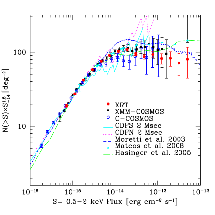
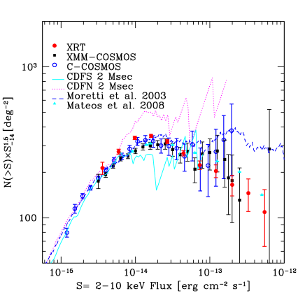
The cumulative number counts in the 0.5-2 keV and 2-10 keV bands are reported in Table 7, while Fig. 12 shows the cumulative number counts normalized to the Euclidean slope ( multiplied by S^1.5); Euclidean number counts would correspond to horizontal lines in this representation. Comparing the XRT number counts in the largest possible flux range, we show in Fig. 12 results from other deep-pencil beam and medium-large shallow surveys. In both the 0.5-2 keV and 2-10 keV bands, one of the major achievements of the XRT survey is the improvement in the knowledge of the bright end number counts. In the 0.5-2 keV band, at fluxes less than $\sim$3-4$\times$10^-14 erg cm^-2 s^-1, the XRT number counts are fully consistent within 1 $\sigma$ errors with previous results. At the brightest fluxes the XRT number counts are systematically lower than the corresponding counts from the largest surveys, which should not suffer cosmic variance as pencil beam or medium area surveys. This systematic behavior can be due to the fact that the XRT catalog includes only point-like sources, thus the number counts do not include the cluster contribution (up to 20-30$\%$ at energy $<$ 2 keV and flux $\geq$10^-13 erg cm^-2 s^-1) unlike the other surveys. In the 2-10 keV band the number counts are consistent within 1 $\sigma$ errors with previous results at medium-deep fluxes. At the brightest fluxes the XRT number counts are slightly lower than the high precision Mateos et al. (2008) number counts, even if they are marginally consistent within 1 $\sigma$ errors. This agreement, unlike the discrepancy in the 0.5-2 keV band, is probably due to the smaller contribution of the clusters at higher energies.

Table 7: Integral number counts and sky coverage in the S and H band (see Sec. 6.2 and 6.3).

Flux (S)	Counts (N$>{\it S}$)	Sky coverage $\Omega_{i}$
$10^{-14}$ ${\rm erg\leavevmode\nobreak\ cm}^{-2}\leavevmode\nobreak\ {\rm s}^{-1}$	deg-2	deg2
0.5-2 keV
50.12	0.2$\pm$0.1	22.12
31.4	0.4$\pm$0.1	22.12
19.68	0.9$\pm$0.2	22.11
12.33	1.9$\pm$0.3	22.11
7.724	4.3$\pm$0.4	22.1
4.839	8.2$\pm$0.6	22.09
3.032	18$\pm$0.9	22.03
1.9	41$\pm$1	21.64
1.19	78$\pm$2	19.57
0.7457	140$\pm$3	16.68
0.4672	237$\pm$4	11.89
0.2927	369$\pm$5	5.73
0.1834	531$\pm$9	1.66
0.1149	703$\pm$17	0.42
0.072	969$\pm$61	0.047
2-10 keV
54.48	0.3$\pm$0.1	22.11
32.98	0.8$\pm$0.2	22.09
19.96	1.8$\pm$0.3	22.06
12.09	4.9$\pm$0.5	21.84
7.316	11.3$\pm$0.7	20.19
4.429	29$\pm$1	17.32
2.681	73$\pm$2	12.28
1.623	169$\pm$4	5.64
0.9824	348$\pm$9	1.51
0.5947	598$\pm$22	0.30
0.36	989$\pm$91	0.02

Figure 12: Cumulative number counts normalized to the Euclidean slope (multiplied by S${}^{1.5}_{-14}$) for HGL sample with detection significance level $\leq$2$\times$10^-5 in the soft band (0.5–2 keV, red filled circles, left panel) and in the hard band (2–10 keV, red filled circles, right panel). Other symbols represent: the C-COSMOS curve (blue open circles, Elvis et al. 2009), the XMM-COSMOS curve (black filled squares, Cappelluti et al. 2009), the Moretti et al. (2003) compilation (blue dashed line), the soft band curve of Hasinger et al. (2005; green dashed line), the CDF-N (magenta dotted line, Alexander et al. 2003) and the CDF-S (cyan solid line, Luo et al. 2008) curves, the Mateos et al. (2008) compilation (cyan solid triangles).

The number counts below $\sim$10 keV were previously best fitted with broken power laws. Following Moretti et al. (2003) we parameterized the integral number counts with two power laws with indices $\alpha_{1}$, which is the slope at the bright fluxes, and $\alpha_{2}$, which is the slope at the faint fluxes, joining without discontinuities at the break flux S₀:

$$N(>S)=K\frac{{(1\times 10^{-14})}^{\alpha_{1}}}{S^{\alpha_{1}}+{S_{0}}^{\alpha_{1}-\alpha_{2}}S^{\alpha_{2}}}\leavevmode\nobreak\ \leavevmode\nobreak\ deg^{-2}$$ (7)

In order to determine the parameters $\alpha_{1}$, $\alpha_{2}$ and S₀ we applied a maximum likelihood algorithm to the differential number counts corrected by the sky coverage (see e.g. Crawford et al. 1970, Murdoch et al. 1973). Although we defined the integral number counts, the method operates on the differential counts, that is the number of sources in each flux range which are independent of each other, unlike the integral number counts. Moreover, using the maximum likelihood method (L_max), the fit is not dependent on the data binning, and therefore we can make full use of the whole data set. The normalization K is not a parameter of the fit, but is obtained by imposing the condition that the number of the expected sources from the best-fit model is equal to the observed total number of sources.

Following Carrera et al. (2007), the 1$\sigma$ uncertainties for $\alpha_{1}$, $\alpha_{2}$ and S₀ are estimated from range of each parameters around the maximum which makes $\Delta$L${}_{max}=$1. For each parameter this is performed by fixing the parameter of interest to a value close to the best fit value and varying the rest of the parameters until a new maximum for the likelihood is found. This procedure is repeated for several values of the parameter until this new maximum equals L${}_{max}+1$.

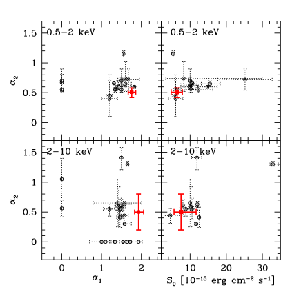
The results of the maximum likelihood fits are given in Table 8 and shown in Fig. 13. We collected results from previous surveys for which a logN-logS fit is available (see Fig. 13). We first note that the logN-logS parameters ($\alpha_{1}$, $\alpha_{2}$, and S₀) are not strongly constrained and sometimes inconsistent of each other. This is probably due to the fact that a good fit would require contemporaneous large flux coverage from the brightest fluxes to the faintest fluxes, and in this case a more detailed model would be necessary. Our best-fit $\alpha_{2}$ are consistent at 1$\sigma$ confidence level with most of the previous results, while our best-fit $\alpha_{1}$ are systematically steeper, especially for the 2-10 keV band. Mainly for the 0.5-2 keV band, this trend, as already noted (see text above), is probably due to the fact that our survey does not contain clusters. The best-fit $\alpha_{1}$ are steeper than the “Euclidean slope” of 1.5 at 1$\sigma$ confidence level, mostly in the 2-10 keV band, probably indicating that some amount of cosmological evolution is present (see also Fig. 12). Also our best-fit S₀ are consistent at 1$\sigma$ confidence level with most of the previous evaluations, further in the 0.5-2 keV band S₀ is better constrained and slightly lower than previously. Note that this is not due to our higher best-fit $\alpha_{1}$, in fact S₀ and $\alpha_{1}$ appear slightly positively correlated (i.e. linear correlation coefficient of $\sim$0.47 and $\sim$0.15 in the S and H band, respectively).

Table 8: LogN-logS best-fit parameters (see eq. 7).

Banda	$\alpha_{1}$b	$\alpha_{2}$c	S0d/10-15	Ke
keV			erg cm-2 s-1	deg-2
0.5-2	1.76${}_{-0.09}^{+0.1}$	0.51${}_{-0.09}^{+0.07}$	6.4${}_{-1.6}^{+1.4}$	154.9
2-10	1.93${}_{-0.10}^{+0.13}$	0.5${}_{-0.3}^{+0.3}$	7.5${}_{-1.9}^{+4.1}$	534.6

^aenergy band;

^bpower law slope for flux $\geq$S₀;

^cpower law slope for flux $<$S₀;

^dflux break;

^enormalization factor.

Unlike the $\chi^{2}$ statistic, the absolute value of L_max is not an indicator of the goodness of fit. Then we analyzed the ratio between the data and the best fit model (see right panel of Fig. 13).We did not find systematic deviations from unity of the ratio, that would indicate that the model is not appropriate to the data.

Figure 13: Left panel: faint spectral index $\alpha_{2}$ vs. the bright spectral index $\alpha_{1}$ for the 0.5-2 keV band and for the 2-10 keV band in the left top and left bottom panel, respectively, and faint spectral index $\alpha_{2}$ vs. the flux break S₀ for the 0.5-2 keV band and for the 2-10 keV band in the right top and right bottom panel, respectively (see text for the definition of $\alpha_{1}$, $\alpha_{2}$ and S₀). The red solid squares are our results for broken power law model, and the black open dots represents a compilation of data from literature: Hasinger et al. 1993, Giommi et al. 2000, Mushotzky et al. 2000, Page et al. 2000, Brandt et al. 2001, Baldi et al. 2002, Cowie et al. 2002, Rosati et al. 2002, Harrison et al. 2003, Moretti et al. 2003, Bauer et al. 2004, Kim et al. 2004, Yang et al. 2004, Hasinger et al. 2005, Kenter et al. 2005, Cappelluti et al. 2007, Brunner et al. 2008, Carrera et al. 2007, Mateos et al. 2008, Ueda et al. 2008, Cappelluti et al. 2009. Right panel: ratio between the binned integral logN-logS and the best fit model in the 0.5-2 keV band (upper panel) and 2-10 keV band (bottom panel). The dotted lines are the ratio between the binned integral logN-logS and predicted 1-$\sigma$ uncertainty interval.

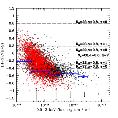
6.4 X-ray spectral properties

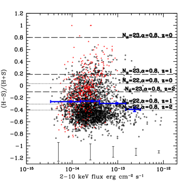
As a first approach, we used the hardness ratio, HR=(c_H-c_S)/($c_{H}$+c_S) (where c_S and c_H are the S and H count rates), to investigate the X-ray spectral properties of the HGL sample. We used the “survival analysis” to take into account the HR lower limits for the S sample and the HR upper limits for the H sample. We find that the H sample shows a mean hardness ratio of $\sim$-0.26, definitively greater than the mean HR of the S sample, which is $\sim$-0.43. Moreover, the mean hardness ratio appears to be anti-correlated with the flux, as in other surveys (see e.g. HELLAS2XMM, Fiore et al. 2003, ELAIS-S1, Puccetti et al. 2006), and in the common flux range the mean HR of the H sample is always greater than the mean hardness ratio of the S sample. Probably this is due to at least two reasons: 1) the contribution of non-AGN sources with very soft X-ray colors decreases as we move to higher energies; 2) higher energies are less biased against absorbed sources, hence we expect more absorbed sources to be detected. We also note that the faintest S sources (see first flux bin in right panel of Fig. 14) have hard X-ray colors consistent with being mildly obscured AGN.
Given that on the one hand the errors on HR are great, and on the other hand the AGN spectrum can be more complex than a simple absorbed power law model (e.g. a soft X-ray extra-component could mimic a lower than real column density), we can roughly evaluate the fraction of obscured sources separating them from the unobscured sources by a threshold value of HR=-0.24, which corresponds to a power-law model absorbed by log N_H$>$21.5, 22.2, 22.7 at z$=$0, 1, 2, respectively (see Hasinger et al. 2003). To take into account sources with only count rate upper limits, we assigned each source a count rate, that is the mean of 10000 random values, drawn from a Gaussian distribution with mean equal to the measured count rate and $\sigma$ equal to the count rate error or drawn from a uniform distribution from zero to the count rate upper limit value at 50% confidence level. We find that the fraction of obscured sources was $\sim$37% and $\sim$15% for the H and S sample, respectively. We also evaluated the fraction of obscured sources in bin of flux (see Fig. 15). The fraction of obscured sources as a function of the flux is consistent within a few % with the results from two other surveys C-COSMOS (Elvis et al. 2009, Puccetti et al. 2009) and ELAIS-S1 (Puccetti et al. 2006), except for the S band, for which at flux $\leq$3$\times 10^{-15}$ erg cm^-2 s^-1 the fraction of obscured SwifFT sources is systematically greater than that of the other two survey. This is probably due to the great number ($\sim 57\%$) of S sources with conservative H upper limits near the survey flux limit, because the S flux limits are deeper than the H flux limits, this effect has an impact in the S band mainly, where a lot of faint sources are not detected in the H band, due to the higher H flux limit. This hypothesis is supported by the fact that the fraction of the obscured C-COSMOS and HELLAS2XMM sources is greater than the fraction of the obscured S SwiftFT sources, evaluated by zeroing the H upper limits (red dotted line in the upper panel of Fig. 15).
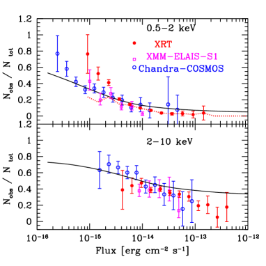
To check whether the theoretical models show a rough agreement with the data, we compared the fraction of the obscured sources, defined by the hardness ratio method, as a function of flux, with those predicted by the X-ray background synthesis model by Gilli et al. 2007. These latter were determined by the POMPA COUNTS tool, using a redshift range of 0-3, a column density range of 10²⁰-10²⁴ cm^-2 and a column density of 10²¹ cm^-2 to distinguish obscured from unobscured sources. The data are generally consistent with the model predictions. The greatest discrepancy between data and model is find in the S band, near the flux limit of each surveys (i.e $\leq$3$\times 10^{-15}$ erg cm^-2 s^-1 for SwiftFT, and $\leq$4$\times 10^{-16}$ erg cm^-2 s^-1 for C-COSMOS), where the data are systematically greater by $\geq$1$\sigma$ than the model. This, as noticed above, is probably due to the great number of the S sources with conservative H upper limits near the survey S flux limit.

Figure 14: Left panel: hardness ratio (see Sec. 6.4) vs. the 2-10 keV flux, for the H HGL sample. The red triangles represent lower limits hardness ratios evaluated using 50% S count rate upper limits. The crosses are the mean hardness ratios in flux bins, evaluated using the “survival analysis” (Kaplan & Meier 1958; Miller 1981, p. 74). The mean 1 $\sigma$ errors in the hardness ratio at different fluxes are indicated by the error bars plotted at the bottom. The dotted and dashed lines show for comparison the hardness ratio for an absorbed power-law model of photon index $\Gamma=$1.8 and column density 10²² cm^-2 and 10²³ cm^-2, respectively, at redshift decreasing from 2 to 0 (from bottom to top). Right panel: hardness ratio (see Sec. 6.4) vs. the 0.5-2 keV flux, for the S HGL sample, here the red triangles are upper limits hardness ratios evaluated using 50% H count rate upper limits. Other symbols like in right panel.

Figure 15: Fraction of obscured sources as a function of the source flux for three surveys: SwiftFT (red solid points), ELAIS-S1 (magenta open points), C-COSMOS (blue open dots). The black solid line represents the X-ray background synthesis model by Gilli et al. 2007. The red dotted line represents the fraction of obscured sources for the SwiftFT survey, by zeroing the flux limits in the hard band. Upper panel: S sample. Lower panel: H sample.

7 Conclusion

We analyzed 374 Swift-XRT fields, 373 of which are Gamma Ray Burst fields, with exposure times ranging from 10 ks to over 1 Ms. Thanks to the long exposure time of the Gamma Ray Burst fields, the spatial isotropy of the Gamma Ray Bursts, the low XRT background, and the nearly constant XRT PSF and vignetting, the SwiftFT can be considered the ideal survey of serendipitous sources without bias towards known targets, with uniform flux coverage, deep flux limit, and large area.

Our main findings are:

• We produced a catalogue including the main X-ray characteristics of the serendipitous sources in the SwiftFT. We analyzed three energy bands S (0.3-3 keV), H (2-10 keV) and F (0.3-10 keV). We detect 9387 distinct point-like serendipitous sources, 7071 of which are at high Galactic-latitude (i.e. $\mid$b$\mid\geq$20 deg.), with a detection significance level $\leq$2$\times$10^-5 in at least one of the three analyzed bands, at flux limits of 7.2$\times 10^{-16}$erg cm^-2 s^-1 ($\sim$4.8$\times 10^{-15}$ erg cm^-2 s^-1 at 50% completeness), 3.4$\times 10^{-15}$ ($\sim$2.6$\times 10^{-14}$ erg cm^-2 s^-1 at 50% completeness), 1.7$\times 10^{-15}$ erg cm^-2 s^-1 in the S, H, and F band, respectively. 90% of the sources have positional error less than 5 arcs, 68% less than 4 arcs.

• The large number of sources and the wide flux coverage allowed us to evaluate the X-ray number counts of the high Galactic sample in the 0.5-2 keV and 2-10 keV bands with high statistical significance in a large flux interval. The XRT number counts are in agreement at 1$\sigma$ confidence level with previous surveys at faint fluxes, and increase the knowledge of poorly known bright end of the X-ray number counts. The integral logN-logS is well fitted (see Fig. 13) with a broken power law with indices $\alpha_{1}$ and $\alpha_{2}$ for the bright and faint parts, and break flux S₀ (see eq. 7). Using a maximum likelihood, we find for the 0.5-2 keV band $\alpha_{1}=1.76_{-0.09}^{+0.1}$, $\alpha_{2}=0.51_{-0.09}^{+0.07}$, S${}_{0}=6.4_{-1.6}^{+1.4}$ 10^-15 erg cm^-2 s^-1, and for the 2-10 keV $\alpha_{1}=1.93_{-0.10}^{+0.13}$, $\alpha_{2}=0.5_{-0.3}^{+0.3}$ and S${}_{0}=7.5_{-1.9}^{+4.1}$ 10^-15 erg cm^-2 s^-1.

  Compared to results from previous surveys, our best-fit $\alpha_{2}$ values are consistent at 1$\sigma$ confidence level, while our best-fit $\alpha_{1}$ values are systematically steeper, especially for the 2-10 keV band. Also our best-fit S₀ values are consistent at 1$\sigma$ confidence level with most of the previous evaluations, further in the 0.5-2 keV band S₀ is better constrained and slightly lower than previously. Mainly for the 0.5-2 keV band, the steeper value of $\alpha_{1}$ is probably due to the fact that our survey does not contain clusters, unlike the other surveys, which contribute up to 20-30$\%$ at energy $<$ 2 keV and flux $\geq$10^-13 erg cm^-2 s^-1. The greater $\alpha_{1}$ and the lower S₀ are not due to an intrinsic anticorrelation of the two parameters in the model. We note a great dispersion of the previous logN-logS parameters (see Fig. 13).

• We used the X-ray colors to roughly study the obscured sources in the HGL sample. From this analysis we find that many sources show X-ray colors consistent with being moderately obscured active galactic nuclei, $\sim$37% and $\sim$15% of the H and S sample, respectively. The fraction of obscured sources is increasing at low X-ray fluxes and at high energies, consistent with the results of other surveys (see e.g. ELAIS-S1, Puccetti et al. 2006, C-COSMOS Elvis et al. 2009). The fraction of obscured sources, defined by the hardness ratio method, is roughly consistent with those predicted by the X-ray background synthesis model by Gilli et al. 2007, using rest frame hydrogen column density to define obscured sources. A more detailed comparison between model and data, will be possible using the sub-sample of 40% of the high Galactic-latitude fields, which have Sloan Sky Digital Survey coverage. For this field an analysis of the optical counterparts is in progress.