The ground state construction of the two-dimensional Hubbard model on
the honeycomb lattice
Alessandro Giuliani
Dipartimento di Matematica, Università di Roma Tre
L.go S. L. Murialdo 1, 00146 Roma, Italy
Abstract
In these lectures I consider the half-filled two-dimensional (2D) Hubbard model
on the honeycomb lattice and I review the rigorous construction of its ground
state properties by making use of constructive fermionic Renormalization Group
methods.
1 Introduction
There are very few quantum interacting systems whose ground state properties
(thermodynamic functions, reduced density matrices, etc.) can be computed
without approximations. Among these, the Luttinger and the Thirring model
To ; Lu ; ML ; Th ; J (one-dimensional spinless relativistic fermions),
the one-dimensional Hubbard model LW ; EFGKK (non-relativistic lattice
fermions with spin), the Lieb-Liniger model LL ; L (one-dimensional bosons
with repulsive delta interactions) and the BCS model BCS ; RS ; DPS
(-dimensional spinning fermions with mean field interactions, );
the construction of the ground states of these systems is based on some
remarkable exact solutions, which make use of bosonization techniques and Bethe
ansatz. Unfortunately, in most cases these exact solutions do not allow to
compute the long-distance decay of the -particles correlation functions
in a closed form (with some notable exceptions, namely the Luttinger and
Thirring models, see K ; Ma ). Moreover, even the computation of the
thermodynamic functions crucially relies on a very special choice of the
particle-particle interaction; as soon as the interparticle potential is
slightly modified the exact solvability of these models is destroyed and no
conclusion on the new “perturbed” system can be drawn from their solution.
This is, of course, very annoying and unsatisfactory from a physical point of
view.
There is another rigorous powerful method that allows in a few cases to fully
construct the ground state of a system of interacting particles,
known as Renormalization Group (RG). This method, whenever it works, has the
advantage that it provides full information on the zero or low temperatures
state of the system, including correlations and that, typically, it is robust
under small modifications of the interparticle potential; even better, it
usually gives a very precise meaning to what “small modifications” means:
it allows one to classify perturbations into “relevant” and “irrelevant”
and to show that the addition of a small irrelevant perturbation does not
change the asymptotic behavior of correlations. Unfortunately, it only works in
the weak coupling regime and it has only been successfully applied to a limited
number of interacting quantum systems. Most of the available results on the
ground (or thermal) states of interacting quantum systems obtained via RG
concern one-dimensional (1D) weakly interacting fermions, e.g., ultraviolet
models with GK ; FMRS , ultraviolet QED-like models
Le and non-relativistic lattice systems BGPS ; GeM ; BM . In more than
one dimension, most of the result derived by rigorous RG techniques concern the
finite temperature properties of two-dimensional (2D) fermionic systems above
the BCS critical temperature BG ; FMRT ; DR1 ; DRprl ; BGM1 ; BGM2 . Two
remarkable exceptions are the Fermi liquid construction by Feldman, Knörrer
and Trubowitz FKT , which concerns zero temperature properties of a
system of 2D interacting fermions with highly asymmetric Fermi surface, and the
ground state construction of the short range half-filled 2D Hubbard model on
the honeycomb lattice by Giuliani and Mastropietro GM10 ; GMprb , which
will be reviewed here.
The 2D Hubbard model on the honeycomb lattice is a basic model for describing
graphene, a newly discovered material consisting of a one-atom thick
layer of graphite N , see CGPNG for a comprehensive and up-to-date review of its
low temperature properties. One of the most remarkable features of graphene is
that at half-filling the Fermi surface is highly degenerate and it consists of
just two isolated points. This makes the infrared properties of the system very
peculiar: in the absence of interactions, it behaves in the same way as a system of
non-interacting -dimensional Dirac particles W . Therefore, the interacting system is a
sort of -dimensional QED, with some peculiar differences that make its study new and
non-trivial Se ; Ha .
The goal of these lectures is to give a self-contained proof of the analyticity of the ground state
energy of the Hubbard model on the 2D honeycomb lattice at half filling and
weak coupling via constructive RG methods. A simple extension of the proof of convergence of the
series for the specific ground
state energy presented below allows one to construct the whole set of reduced density matrices
at weak coupling (see GM10 ): it turns out that the off-diagonal elements of these matrices
decay to zero at infinity, with the same decay exponents as the non-interacting system; in this
sense, the construction presented below rigorously exclude the presence of long range order
in the ground state, and the absence of anomalous critical exponents (in other words,
the interacting system is in the same universality class as the non-interacting one). Let me also
mention that more sophisticated extensions of the methods exposed here also allowed us to: (i) give an
order by order construction of the ground state correlations of the same model in the presence of
electromagnetic interactions GMP1 ; GMP2 ; (ii) predict a possible mechanism for the
spontaneous generation of the Peierls-Kekulé instability GMP2 ; (iii) prove the universality of
the optical conductivity GMP3 .
The plan of these lectures is the following:
•
In Section 2, I introduce the model and state the main result.
In Section 4, I describe the formal series expansion for the
ground state energy, I explain how to conveniently re-express it in terms of Grassmann
functional integrals and estimate by naive power-counting the generic
-th order in perturbation theory, so identifying two main issues in the convergence of the
series: a combinatorial problem, related to the large number of Feynman graphs contributing at
a generic perturbative order, and a divergence problem, related to the (very mild) ultraviolet
singularity of the propagator and to its (more serious) infrared singularity.
•
In Section 5, I describe a way to reorganize and estimate the
perturbation theory, via the so-called determinant expansion, that allows one to prove
convergence of the series, for any fixed choice of the ultraviolet and infrared cut-offs.
•
In Section 6, I describe how to resum the determinant expansion in order
to cure the mild ultraviolet divergences appearing in perturbation theory, via a multiscale
expansion, whose result is conveniently expressed in terms of Gallavotti-Nicolò trees
GN ; G .
•
In Section 7, I describe how to resum and cure the infrared divergences
and conclude the proof of the main result.
•
Finally, in Section 8, I draw the conclusions. A few technical aspects of the proof are
described in the Appendixes
The material presented in this lectures is mostly taken from GM10 . Some technical proofs
concerning the determinant and the tree expansions are taken from the review
GeM . Other reviews of the constructive RG methods discussed here, which the reader
may find useful to consult, are BGbook ; G ; M2 ; Sa .
2 The Model and the Main Results
The grandcanonical
Hamiltonian of the 2D Hubbard model on the honeycomb lattice at half
filling in second quantized form is given by:
is a periodic triangular lattice, defined as
, where and 𝔹 is the infinite triangular
lattice with basis
, . is obtained by translating by a nearest neighbor vector , , where
The honeycomb lattice we are interested in
is the union of the two triangular sublattices and , see Fig.1
Figure 1:
A portion of the honeycomb lattice . The white and black dots correspond
to the sites of the and triangular sublattices, respectively. These two
sublattices are one the translate of the other. They are connected by nearest neighbor vectors
that, in our units, are of unit length.
2.
are creation or annihilation
fermionic operators with spin index and
site index , satisfying periodic boundary conditions
in . Similarly,
are creation or
annihilation
fermionic operators with spin index and
site index ,
satisfying periodic boundary conditions in .
3.
is the strength of the
on–site density–density interaction;
it can be either positive or negative.
Note that the terms in the second line of Eq.(2.1)
can be rewritten as the sum of a truly quartic term in the creation/annihilation operators (the density-density interaction), plus a quadratic term (a chemical potential term, of the form ,
with the chemical potential and the total particles number operator), plus a constant
(which plays no role in the thermodynamic properties of the system).
The Hamiltonian (2.1) is hole-particle symmetric,
i.e., it is invariant under the exchange , . This invariance implies in particular that, if
we define the average density of the system to be
, with the total particle number operator and
the average with respect to the (grandcanonical) Gibbs
measure at inverse temperature , one has , for any
and any ; in other words, the grand-canonical Hamiltonian Eq.(2.1)
describes the system at half-filling, for all . Let
be the specific free energy of the system and
the specific ground state energy. We will prove the following
Theorem.
Theorem 2.1
There exists a constant such that, if , the specific
free energy of the 2D Hubbard model on the honeycomb lattice at half filling is an
analytic function of , uniformly in as
, and so is the specific ground state energy .
The proof is based on RG methods, which will be reviewed below. A straightforward extension
of the proof of Theorem 2.1 allows one to prove that the correlation functions (i.e., the
off-diagonal elements of the reduced density matrices of the system) are analytic functions
of and they decay to zero at infinity with the same decay exponents as in the non-interacting
() case, see GM10 . This rigorously excludes the presence of LRO in the ground state
and proves that the interacting system is in the same universality class as the non-interacting
system.
3 The non-interacting system
Let us begin by reviewing the construction of the finite and zero temperature states for the
non-interacting () case.
In this case the Hamiltonian of interest reduces to
with , , defined
as in items (1)–(4) after (2.1). We aim at computing the spectrum of by
diagonalizing the right hand side (r.h.s.) of (3.1). To this purpose, we pass
to Fourier space.
We identify the periodic triangular lattice with the set of vectors of the infinite triangular lattice
within a “box” of size , i.e.,
and footnote .
With the previous definitions, we can rewrite
with the unperturbed Fermi velocity (if the hopping strength is chosen
to be the one measured in real graphene, turns out to be approximately 300 times
smaller than the speed of light) and
the complex dispersion relation. By looking at the second line of Eq.(3),
one realizes that the natural creation/annihilation operator is a 2D spinor of components
and :
In order to fully diagonalize the theory, one needs to perform the diagonalization of the
quadratic form in the second line of Eq.(3), which can be realized by the
-dependent unitary transformation
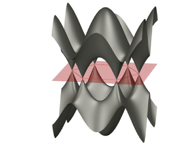
Figure 2:
A sketch of the energy bands of the free electron gas with nearest neighbor hopping
on the honeycomb lattice. The red plane corresponds to the Fermi energy at half-filling. It cuts the
bands at a discrete set of points, known as the Fermi points or Dirac points. From the picture, it seems that there are six distinct Fermi points. However, after identification of the points modulo
vectors of the reciprocal lattice, it turns out that only two of them are independent.
They cross the Fermi energy at the Fermi points ,
, with
resembling in this sense the relativistic dispersion relation of -dimensional Dirac fermions.
From Eq.(3) it is apparent that the ground state of the system consists of a Fermi sea
such that all the negative energy states (the “-states”) are filled and all the positive energy
states (the “-states”) are empty. The specific ground state energy is
Besides these thermodynamic functions, it is also useful to compute the Schwinger
functions of the free gas, in terms of which, in the next section, we will write down the perturbation
theory for the interacting system. These are defined as follows.
Let be an imaginary time, let and let us
consider the time-evolved operator , where is the two-components spinor defined in Eq.(3.16); in the following we shall denote its components by
, with ,
and (here ).
We define the -points Schwinger functions
at finite volme and finite temperature as:
where is a permutation of , chosen in such a
way that , and is its
sign. [If some of the time coordinates are
equal each other, the arbitrariness of the definition is solved by
ordering each set of operators with the same time coordinate so
that creation operators precede the annihilation operators.]
Taking the limit in (3.26) we get the finite
temperature -point Schwinger functions, denoted by
,
which describe the properties of the infinite volume system at
finite temperature. Taking the limit of the finite
temperature Schwinger functions, we get the zero temperature
Schwinger functions, simply denoted by
, which
by definition characterize the properties of the thermal ground state
of (2.1) in the thermodynamic limit.
In the non-interacting case, i.e., if , the Hamiltonian is quadratic in the
creation/annihilation operators. Therefore, the -point
Schwinger functions satisfy the Wick rule, i.e.,
Moreover, every –point
Schwinger function with
is identically zero. Therefore, in order to construct the whole set of
Schwinger functions of , it is enough to compute the –point
function . This can be easily reconstructed from the
2-point function of the -fields and -fields, see Eq.(3.18).
Let , and ; if , let
and . A straightforward computation
shows that, if ,
and . A priori,
Eqs.(3) and (3) are defined only for
, but we can extend them periodically over the
whole real axis; the periodic extension of the propagator is
continuous in the time variable for , and it has
jump discontinuities at the points .
Note that at , the difference between the right and left
limits is equal to
, so that the propagator is discontinuous only
at . If we define ,
with , then
for we can write
Let us now turn to the interacting case. The first step is to derive a formal
perturbation theory for the specific free energy and ground state energy. In other words, we want
to find rules to compute the generic perturbative order in of . We write , with the operator
in the second line of Eq.(2.1) and we use Trotter’s product formula
and must be interpreted as .
Note that the -th term in the sum in the r.h.s. of Eq.(4.3) can be computed by
using the Wick rule (3.28) and the explicit expression for the 2-point function
Eqs.(3.33)-(3.34). It is straightforward to check that the “Feynman rules” needed
to compute are the following:
(i) draw graph elements consisting of
4-legged vertices, with the vertex associated to two labels and , , and
the four legs associated to two exiting fields (with labels and
) and two entering fields (with labels and
), respectively;
(ii) pair the fields in all possible ways, in such a way that every pair consists of one entering and
one exiting field, with the same spin index, see Fig.3;
Figure 3: The four-legged graph element (left); an example of a Feynman
diagram of order 3 (right).
(iii) associate to every pairing a sign, corresponding to
the sign of the permutation needed to bring every pair of contracted fields next to each other;
(iv) associate to every paired pair of fields
an oriented line connecting the -th with the -th vertex, with orientation from to ;
(v) associate to every oriented line a value equal to
where , and is a smooth compact support function that
is equal to 1 for (say) and equal to 0 for ; (vi) associate to every pairing
(i.e., to every Feynman graph) a value, equal to the product of the sign of the pairing times
times the product of the values of all the oriented
lines; (vii) integrate over and sum over the value of each pairing, then sum over
all pairings; (viii) finally, take the limit:
the result is equal to . Note that the limit
of the propagator is equal to if , while
, see Eq.(3.34): the difference
between and takes into account the terms in
the definition of .
An algebraically convenient way to re-express Eq.(4.3) is in terms of
Grassmann integrals. Consider the set , where the Grassmann variables
satisfy by the definition the anticommutation rules
.
In particular, the square of a Grassmann
variable is zero and the only non-trivial Grassmann monomials
are at most linear in each variable. Let the Grassmann algebra generated by
be the set of all polynomials obtained by linear combinations of such
non-trivial monomials. Let us also define the Grassmann
integration as
the linear operator on the Grassmann algebra such that, given a
monomial in the variables
, its action on is except in the case , up to a permutation of the variables. In
this case the value of the integral is determined, by using the
anticommutation properties of the variables, by the condition
while the average of an arbitrary monomial in the Grassmann variables with respect
to is given by the fermionic Wick rule with propagator equal to the r.h.s. of
Eq.(4.9). Using these definitions and the Feynman rules described above, we can rewrite
Eq.(4.3) as
and the exponential in the r.h.s. of Eq.(4.10) must be identified with its
Taylor series in (which is finite for every finite , due to the anticommutation rules of the
Grassmann variables and the fact that the Grassmann algebra is finite for every finite ).
Apriori, Eq.(4.10) must be understood as an equality between formal power series in .
However, it can be given a non-perturbative meaning, provided that we can prove
the convergence of the Grassmann functional integral in the r.h.s., as shown by the following Proposition.
under the given analyticity assumptions on .
The first key remark is that, if are finite, the left hand side of
Eq.(4.15) is a priori well defined and analytic on the whole complex
plane. In fact, by the Pauli principle, the Fock space generated by the fermion
operators , with
, is finite dimensional.
Therefore, writing , with and
two bounded operators, we see that is an
entire function of , simply because converges
in norm over the whole complex plane:
where the norm is, e.g., the Hilbert-Schmidt norm .
On the other hand, by assumption, is analytic in
, with independent of , and uniformly
convergent as . Hence, by Weierstrass theorem, the limit
is analytic in
and its Taylor coefficients coincide with the limits as
of the Taylor coefficients of . Moreover,
,
again by Weierstrass theorem.
As discussed above, the Taylor coefficients of
coincide with the Taylor coefficients of : therefore,
in the complex region , simply because the l.h.s. is entire
in , the r.h.s. is analytic in and the Taylor coefficients
at the origin of the two sides are the same. Taking logarithms at both sides
proves Eq.(4.14).
By Proposition 4.1, the Grassmann integral Eq.(4.13) can be used to compute the free
energy of the original Hubbard model, provided that the r.h.s. of
Eq.(4.13) is analytic in a domain that is uniform in and that it converges to
a well defined analytic function uniformly as . The rest of these notes are devoted
to the proof of this fact. We start from Eq.(4.13), which can be rewritten as
where the second sum in the r.h.s. runs over partitions of of multiplicity ,
i.e., over -ples of disjoint sets such that ,
with . Note that
can be computed as a sum of
Feynman diagrams whose values are determined by the same Feynman rules described after
Eq.(4.4) (with the exception of rule (viii): of course, since ,
should be temporarily kept fixed in the computation); we shall write
where is the set of all Feynman diagrams with vertices,
constructed with the rules described above; includes the integration over
the space-time labels and the sum over the component labels : if ,
we shall write symbolically
where is the sign of the permutation associated to the graph and
we denoted by and
the labels of the two vertices, which the line exits from and enters in, respectively.
Using Eqs.(4.20)-(4.21), it can be proved by induction that
where is the set of connected Feynman diagrams
with vertices. Combining Eq.(4.17) with Eq.(4.23) we finally have a
formal power series expansion for the specific free energy of our model (more precisely, of its
ultraviolet regularization associated to the imaginary-time ultraviolet cutoff ).
The Feynman rules for computing allow us to derive a first very naive
upper bound on the -th order contribution to , that is to
where is the number of connected Feynman diagrams of order
and is a uniform bound on the value of a generic
connected Feynman diagram of order . The bound is obtained as follows: given
, select an arbitrary “spanning tree” in , i.e. a loopless subset
of that connects all the vertices; now: the integrals over the space-time
coordinates of the product of the propagators on the spanning tree can be bounded
by ; the product of the remaining propagators can be bounded by
; finally, the sum over the labels is bounded by .
Using Eq.(4.25) and the facts that, for a suitable constant :
(i) (see, e.g., (GeM, , Appendix A.1.3) for a proof of this fact),
(ii) , (iii) , we find:
Remark. While the bound (see Appendix A for a proof) is dimensionally optimal,
the estimate could be improved to , at the cost
of a more detailed analysis of the definition of , which shows that the apparent
ultraviolet logarithmic divergence associated to the sum over in Eq.(4.5)
is in fact related to a jump singularity of at . This can be proved
along the lines of (Be, , Section 2). However, to the purpose of the present discussion,
the rough (and easier) bound is enough; see Appendix A for a proof.
The pessimistic bound Eq.(4.26) has two main problems: (i) a combinatorial problem,
associated to the , which makes the r.h.s. of Eq.(4.26) not summable over , not
even for finite and ; (ii) a divergence problem, associated to
the factor , which diverges exponentially as (i.e., as
the ultraviolet regularization is removed) and as (i.e., as the temperature is sent to 0).
The combinatorial problem is solved by a smart reorganization of the perturbation theory, in the
form of a determinant expansion, together with a systematic use of the Gram-Hadamard bound.
The divergence problem is solved by systematic resummations of the series: we will first identify
the class of contributions that produce ultraviolet or infrared divergences
and then we show how to inductively resum them into a redefinition of the coupling constants of
the theory; the inductive resummations are based on a multiscale integration of the theory: at the
end of the construction, they will allow us to express the specific free energy in terms of modified
Feynman diagrams, whose values are not affected anymore by ultraviolet or infrared divergences.
5 The determinant expansion
Let us now show how to attack the first of two problems that arose at the end of previous section.
In other words, let us show how to solve the combinatorial problem by reorganizing the
perturbative expansion discussed above into a more compact and more convenient form.
In the previous section we discussed a Feynman diagram representation of the truncated
expectation, see Eq.(4.23). A slightly more general version of
Eq.(4.23) is the following. For a given set of indices , with
, , let
Each field can be represented as an oriented
half-line, emerging from the point and carrying an arrow, pointing in the direction entering
or exiting the point, depending on whether is equal to or , respectively; moreover,
the half-line carries two labels, and .
Now, given set of indices , we can enclose the points belonging
to the set , for some , in a box: in this way, assuming that all the points ,
, are distinct, we obtain disjoint boxes. Given ,
we can associate to it the set of connected Feynman diagrams, obtained by
pairing the half-lines with consistent orientations, in such a way that the two half-lines of any
connected pairs carry the same spin index, and in such a way that all the boxes are connected.
Using a notation similar to Eq.(4.22), we have:
any element of the set is a set of lines forming an anchored tree between
the boxes , i.e., is a set
of lines that becomes a tree if one identifies all the points
in the same clusters;
•
is a sign (irrelevant for the subsequent bounds);
•
is a shorthand for ;
•
if , then
is a probability measure with support on a set of such that
for some family of vectors of
unit norm;
•
if , then
is a matrix, whose
elements are given by , where:
and are
the two field labels associated to the two (entering and exiting) half-lines contracted into ;
is s.t. ; is the propagator associated to the line
obtained by contracting the two half-lines with indices and .
If the sum over is empty, but we can still
use the Eq.(5.3) by interpreting the r.h.s.
as equal to if is empty and equal to otherwise.
The proof of the determinant representation is described in Appendix B;
this representation is due to a fermionic reinterpretation
of the interpolation formulas by Battle, Brydges and Federbush BF ; B ; BrF ,
used originally by Gawedski-Kupianen GK and by Lesniewski Le , among others,
to study certain -dimensional fermionic Quantum Field Theories. Using
Eq.(5.3) we get an alternative representation for the -th order contribution to
the specific free energy:
Using the fact that the number of anchored trees in is bounded by for a
suitable constant (see, e.g., (GeM, , Appendix A.3.3) for a proof of this fact),
from Eq.(5.4) we get:
In order to bound , we use the Gram-Hadamard inequality, stating
that, if is a square matrix with elements of the form
, where , are vectors in a Hilbert space with
scalar product , then
where is the norm induced by the scalar product. See (GeM, , Theorem A.1)
for a proof of Eq.(5.6).
Let , where is the Hilbert space of the
functions ,
with scalar product ,
where , , , are the components of the vectors
and . It is easy to verify that
which is similar to Eq.(4.26), but for the fact that there is no in the r.h.s.! In other words,
using the determinant expansion, we recovered the same dimensional estimate as the one
obtained by the Feynman diagram expansion and we combinatorially gained a .
The r.h.s. of Eq.(5.10) is now summable over for sufficiently small,
even though non uniformly in and . In the next section we will discuss how to
systematically improve the dimensional bound by an iterative resummation method.
6 The multiscale integration: the ultraviolet regime
In this section we begin to illustrate the multiscale integration of the fermionic
functional integral of interest. This method will later allow us to perform iterative resummations
and to re-express the specific free energy in terms of a modified expansion, whose -th order
term is summable in and uniformly convergent as and , as desired.
The first step in the computation of the partition function
and of its logarithm is the integration of the ultraviolet degrees of freedom
corresponding to the large
values of . We proceed in the following way. We decompose the free
propagator into a sum of two propagators supported in
the regions of “large” and “small”, respectively. The
regions of large and small are defined in terms of the smooth
support function introduced after Eq.(4.5); note that, by the very definition
of , the supports
of and
are disjoint (here
is the euclidean norm over ). We define
Similarly to , the Gaussian integrations , also admit an explicit
representation analogous to (4.8), with replaced
by or and the sum
over restricted to the values in the support of or
, respectively. The definition of Grassmann integration
implies the following identity (“addition principle”):
with a basis of .
The possibility of representing in the form
(6.8), with the kernels independent of the
spin indices , follows from a number of remarkable symmetries, discussed
in Appendix C, see in particular symmetries (1)–(3) in Lemma C.1.
The regularity properties of the kernels are summarized in the
following Lemma, which will be proved below.
Lemma 6.1The constant in (6.6) and the kernels in
(6.8) are
given by power series in , convergent
in the complex disc , for small enough and independent of
; after Fourier
transform, the -space counterparts of the kernels
satisfy the following bounds:
for some constant .
Moreover, the limits and
exist and are reached uniformly in , so that,
in particular, the limiting functions are analytic in the same domain and so are their limits
(that, with some abuse of notation, we shall denote by the same symbols).
Remark.
Once that the ultraviolet degrees of freedom have been integrated out, the
remaining infrared problem (i.e., the computation of the Grassmann integral
in the second line of Eq.(6.6)) is essentially independent of ,
given the fact that the limit of the kernles
is reached uniformly and that
the limiting kernels are analytic and satisfy the same bounds as Eq.(6.10).
For this reason, in the infrared integration described in the next two
sections, will not play any essential role and, whenever possible, we will
simplify the notation by dropping the label .
Before we present the proof of Lemma 6.1, let us note that the kernels
satisfy a number of non-trivial invariance properties. We will be particularly interested in the invariance
properties of the quadratic part , which will
be used below to show that the structure of the
quadratic part of the new effective interaction has the same symmetries
as the free integration. The crucial properties that we will need are summarized in the following
Lemma, which is proved in Appendix C.
Lemma 6.2.The kernel , thought as a matrix with components ,
satisfies the following symmetry properties:
Note that Eq.(6.12) can be read by saying that, in the zero temperature
and thermodynamic limits, the two-legged kernel has the same structure as
the inverse of the free covariance, , modulo higher order terms in
. This fact will be used in the next section to define a dressed infrared
propagator , with the same infrared singularity structure as the free one. We will come back to this point in more detail. For the moment, let us turn to the proof of Lemma 6.1, which illustrates the main RG strategy
that will be also used below, in the more difficult infrared integration.
Proof of Lemma 6.1.
Let us rewrite
the Fourier transform of as
where
is the distance over the one-dimensional
torus of length and
is the distance over the periodic lattice
(here 𝔹 is the triangular lattice defined after Eq.(2.1));
see Appendix A for a proof. Moreover,
admits a Gram representation that, in notation analogous to Eq.(5.7), reads
where is the fermionic “Gaussian integration”
associated with the propagator
(i.e., it is the same as ); moreover, we want to prove that
and are uniformly convergent as .
We perform the integration of (6.19) in an iterative fashion: in fact,
we will inductively prove that for ,
Eq.(6.25) can be graphically represented as in Fig.4.
Figure 4: The graphical representation of .
The tree in the l.h.s., consisting of a single horizontal branch, connecting the
left node
(called the root and associated to the scale label )
with a big black dot on scale , represents . In the r.h.s.,
the term with final points represents the corresponding term in
the r.h.s. of Eq.(6.25): a scale label
is attached to the leftmost node (the root); a scale label
is attached to the central node (corresponding to the action of );
a scale label is attached to the rightmost nodes with the big black dots
(representing ). Iterating the graphical equation in Fig.4 up to scale
, and representing the endpoints on scale as simple dots (rather than big black dots),
we end up with a graphical representation of in terms of Gallavotti-Nicolò
trees, see Fig.5, defined in terms of the following features.
Figure 5: A tree with :
the root is on scale and the
endpoints are on scale .
1.
Let us consider the family of all trees which can be constructed
by joining a point , the root, with an ordered set of
points, the endpoints of the unlabeled tree,
so that is not a branching point. will be called the
order of the unlabeled tree and the branching points will be called
the non trivial vertices.
The unlabeled trees are partially ordered from the root
to the endpoints in the natural way; we shall use the symbol
to denote the partial order.
Two unlabeled trees are identified if they can be superposed by a suitable
continuous deformation, so that the endpoints with the same index coincide.
It is then easy to see that the number of unlabeled trees with end-points
is bounded by (see, e.g., (GeM, , Appendix A.1.2) for a proof of this fact).
We shall also consider the labelled trees (to be called
simply trees in the following); they are defined by associating
some labels with the unlabelled trees, as explained in the
following items.
2.
We associate a label with the root and we denote by
the corresponding set of labeled trees with
endpoints. Moreover, we introduce a family of vertical lines,
labeled by an integer taking values in , and we represent
any tree so that, if is an endpoint, it is contained
in the vertical line with index , while if it is a non trivial vertex,
it is contained in a vertical line with index
, to be called the scale of ; the root is on
the line with index .
In general, the tree will intersect the vertical lines in set of
points different from the root, the endpoints and the branching
points; these points will be called trivial vertices.
The set of the vertices will be the union of the endpoints, of the trivial
vertices and of the non trivial vertices; note that the root is not a vertex.
Every vertex of a
tree will be associated to its scale label , defined, as
above, as the label of the vertical line whom belongs to. Note
that, if and are two vertices and , then
.
3.
There is only one vertex immediately following
the root, called and with scale label equal to .
4.
Given a vertex of that is not an endpoint,
we can consider the subtrees of with root , which correspond to the
connected components of the restriction of
to the vertices . If a subtree with root contains only
and one endpoint on scale ,
it will be called a trivial subtree.
5.
With each endpoint we associate a factor
and a set of space-time
points (the corresponding integration variables in the -space
representation).
6.
We introduce a field label to distinguish the field variables
appearing in the factors associated with the endpoints;
the set of field labels associated with the endpoint will be called ;
note that if is an endpoint . Analogously, if is not an endpoint, we shall
call the set of field labels associated with the endpoints following
the vertex ; , , and will denote the
space-time point, the index, the index and the index,
respectively, of the Grassmann field variable with label .
In terms of trees, the effective potential ,
(with identified with
), can be written as
where and, if is a trivial subtree with root on scale , then .
For what follows, it is important to specify the action of the truncated expectations on the
branches connecting any endpoint to the closest non-trivial vertex
preceding it. In fact, if has only one end-point,
it is convenient to rewrite as:
Now, the key observation is that, since is defined as in Eq.(4.11) and
since our explicit choice of the ultraviolet cutoff makes the tadpoles equal to zero
(i.e., ), then the second term in the r.h.s. of Eq.(6.28)
is identically zero:
for all . Therefore, it is natural to shrink all the branches of
consisting of a subtree , having root on scale
and only one endpoint on scale , into a trivial subtree, rooted in and associated
to the factor . By doing so, we end up with an alternative representation of the
effective potentials, which is based
on a slightly modified tree expansion. The set of modified trees with endpoints contributing
to will be denoted by ; every is characterized
in the same way as the elements of , but for two features:
(i) the endpoints of are not necessarily on scale ; (ii) every endpoint
of is attached to a non-trivial vertex on scale and is
associated to the factor . See Fig.6.
Figure 6: A tree with : the root is on scale and the
endpoints are on scales .
and, if is a trivial subtree with root on scale , then
.
Using its inductive definition Eq.(6.31), the right hand side of Eq.(6.30) can be
further expanded (it is a sum of several contributions, differing for the choices of the
field labels contracted under the action of the truncated expectations
associated with the vertices that are not endpoints), and in order to describe the resulting
expansion we need some more definitions (allowing us to distinguish the fields that are
contracted or not “inside the vertex ”).
We associate with any vertex of the tree a subset of ,
the external fields of . These subsets must satisfy various
constraints. First of all, if is not an endpoint and
are the vertices immediately following it, then
; if is an endpoint, .
If is not an endpoint, we shall denote by the
intersection of and ; this definition implies that . The union of the subsets
is, by definition, the set of the internal fields of ,
and is non empty if .
Given , there are many possible choices of the
subsets , , compatible with all the constraints. We
shall denote by the family of all these choices and by
the elements of . With these definitions, we can rewrite
as:
where has a definition
similar to Eq.(6.33). Moreover, if is an endpoint
; if is not an
endpoint, ,
where . Using in the r.h.s. of Eq.(6.34) the
determinant representation of the truncated expectation discussed in the previous section,
we finally get:
and is a matrix analogous to the one defined in previous section,
with replaced by . Note that and, therefore,
do not depend on : therefore, the effective potential depends on only
through the choice of the scale labels (i.e., the dependence on is all
encoded in ). Using Eqs.(6.35)-(6.36), we finally get the bound:
Now, an application of the Gram–Hadamard inequality Eq.(5.6), combined with
the representation Eq.(6.16) and the dimensional bounds Eq.(6.18), implies that
where, by construction, we have that for any vertex of
that is not an endpoint (simply because every endpoint
of is attached to a non-trivial vertex on scale , see the discussion after
Eq.(6.29)). Now, the number of terms in can be bounded by
(see (GeM, , Appendix A.3.3)); moreover, and , so that
. Therefore,
which implies Eq.(6.10). The constant can be bounded by the r.h.s.
of Eq.(6.37) with and (because the contributions to
with are zero, by the condition that the tadpoles vanish), which implies
Therefore, is given by an absolutely convergent
power series in , as desired. A critical analysis of the proof shows that all the bounds
are uniform in and all the expressions involved admit well-defined limits as
. In particular, this implies that is analytic in (and so is its limit, which is reached
uniformly) in the complex domain , for small enough.
See (GM10, , Appendices C and D) for details on
these technical aspects. This concludes the proof of Lemma 6.1.
We proceed in an iterative fashion, similar to the one described in the previous section
for the integration of the large values of .
As a starting point, it is convenient to decompose the infrared
propagator as:
It is apparent that the field
has zero mass (i.e., its propagator
decays polynomially at large distances in -space). Therefore,
its integration requires an infrared multiscale analysis. As in the analysis
of the ultraviolet problem, we define a sequence of geometrically
decreasing momentum scales , with Correspondingly
we introduce compact support functions and we rewrite
with (the reason why the sum in Eq.(7.9)
runs over is that, if and ,
then , simply because ).
The purpose is to perform the integration of (7.5) in an iterative way.
We step by step decompose the
propagator into a sum of two propagators, the first supported on
momenta , , the second supported
on momenta smaller than . Correspondingly we rewrite the
Grassmann field as a sum of two independent fields: and we integrate the field
. In this way
we inductively prove that, for any , Eq.(7.5) can be
rewritten as
Note that the field ,
whose propagator is given by , has the same support as , that is on a
neighborood of size around the singularity (that, in the
original variables, corresponds to the Dirac point ). It is
important for the following to think , ,
as functions of the variables . The iterative
construction below will inductively imply that the dependence on these
variables is well defined. The iteration continues up to the scale
and the result of the last iteration is .
Localization and renormalization.
In order to inductively prove Eq.(7.10)
we write
and is given by Eq.(7.11) with
replaced by , that is it contains
only the monomials with four fermionic fields or more.
The symmetries of the action, which are described in Appendix C and
are preserved by the iterative integration procedure, imply that, in the zero
temperature and thermodynamic limit,
for suitable real constants . Eq.(7.14) is the analogue of Eq.(6.12); its
proof is completely analogous to the proof of Lemma 6.2 and will not be belabored here.
Once that the above definitions are given, we can describe our iterative
integration procedure for . We start from Eq.(7.10)
and we rewrite it as
Now we can perform the integration of the field.
We rewrite the Grassmann field as a sum of two independent
Grassmann fields and correspondingly we rewrite
Eq.(7.17) as
where
is the truncated expectation of order w.r.t. the
propagator , which is the analogue of Eq.(6.7)
with replaced by and with
replaced by .
Note that the above procedure allows us to write the
effective constants , ,
in terms of , , namely
and ,
where is the so–called Beta function.
An iterative implementation of Eq.(7.27) leads to a representation of
, , in terms of a new tree expansion. The
set of trees of order contributing to is denoted by .
The trees in are defined in a way very similar to
those in , but for the following differences:
(i) all the endpoints are on scale ;
(ii) the scale labels of the vertices of are between and ;
(iii) with each endpoint we associate one of the monomials
with four or more Grassmann fields contributing to , corresponding to the terms with
in the r.h.s. of Eq.(7.6) (here is the linear operator acting as
the identity on Grassmann monomials of order 4 or more, and acting as 0 on Grassmann
monomials of order 0 or 2). In terms of these trees, the effective potential
, , can be written as
where, if is trivial, then and .
Repeating step by step the discussion leading to Eqs.(6.32),(6.35) and (6.36),
and using analogous definitions, we find that
Once again, it is important to note that is a Gram matrix, i.e.,
defining and
,
the matrix elements in Eq.(7.32), using a notation similar to Eq.(5.7),
can be written in terms of scalar products:
Using the representation Eqs.(7.28),(7.29),(7.31)
and proceeding as in the proof of Lemma 6.1, we can get a bound on the kernels of the
effective potentials, which is the key ingredient for the proof of Theorem 2.1 and is
summarized in the following theorem.
Theorem 7.1
There exists a constants , independent
of , and , such that the kernels
in Eq.(7.11), ,
are analytic functions of
in the complex domain ,
satisfying, for any and a suitable constant
(independent of ), the following estimates:
Moreover, the constants and defined by Eq.(7.18)
and Eq.(7.27) are analytic functions of in the same domain ,
uniformly bounded as . Both the kernels
and the constants admit
well defined limits as , which are reached uniformly
(and, with some abuse of notation, will be denoted by the same symbols).
Before we present its proof, let us show how Theorem 7.1 implies, as a corollary,
Theorem 2.1. It is enough to observe that, by Proposition 4.1 and by the
multiscale integration procedure described above,
, with analytic functions of for small enough
(see the discussion at the end of Section 6 and the statement of Theorem 7.1).
Since , the sum is absolutely convergent, uniformly in ; therefore, both
and its limit are analytic functions of for small enough.
This concludes the proof of Theorem 2.1.
Proof of Theorem 7.1.
Let us preliminarily assume that, for ,
and for suitable constants , the corrections
and defined in Eq.(7.14) and Eq.(7.16), satisfy the following
estimates:
for all and a suitable constant . Using the tree expansion described above and,
in particular, Eqs.(7.28),(7.30),(7.31),
we find that the l.h.s. of Eq.(7.36) can be bounded from above by
where is a tree graph
obtained from , by adding
in a suitable (obvious) way, for each endpoint ,
, one or more lines connecting the space-time points
belonging to .
An application of the Gram–Hadamard inequality Eq.(5.6), combined with
the representation Eq.(7.33) and the dimensional bound Eq.(7.35),
implies that
Let us recall that is the number of endpoints following
on , that is the vertex immediately preceding on and that
is the number of field labels associated to the endpoints following
on (note that ). Using the following relations, which can be easily proved by
induction,
Note that, if is not an endpoint, by the
definition of . Now, note that
the number of terms in can be bounded by
. Using also that and ,
we find that the l.h.s. of Eq.(7.49) can be bounded as
which can be bounded via the same strategy as the proof of Eq.(6.10), yielding
Eq.(7.37) for . Similarly,
assuming that Eq.(7.37) is valid for all , the quantities of interest for
can be bounded by
The same proof leading to Eq.(7.51) shows that the r.h.s. of Eq.(7.54)
can be bounded by the r.h.s. of Eq.(7.51) times (that is
the dimensional estimate for ), and that
the r.h.s. of Eq.(7.54)
can be bounded by the r.h.s. of Eq.(7.51) times
(where is the dimensional estimate for ).
It remains to prove the estimates on . The bound on
is an immediate corollary of the discussion above, simply because
can be bounded by Eq.(7.40) with . Finally, remember that
is given by Eq.(7.18): an explicit computation of and the use of
Eqs.(7.37)-(7.38) imply that , from which:
, as desired. This concludes the proof of Theorem 7.1 and, therefore, as discussed after the statement of Theorem 7.1,
it also concludes the proof of analyticity of the specific free energy and ground state energy.
8 Conclusions
In conclusion, I presented a self-contained proof of the analyticity of the specific
free energy and ground state energy of the 2D Hubbard model on the honeycomb lattice,
at half-filling and weak coupling. The proof is based on rigorous
fermionic RG methods and can be extended to the construction of the interacting correlations,
i.e., the off-diagonal elements of the reduced density matrices of the system GM10 ,
and to the computation of the universal optical conductivity GMP3 . Such construction
shows that the interacting correlations decay to zero at infinity with the same decay exponents as
those of the non-interacting case. The “only” effect of the interactions is to change by a finite
amount the quasi-particle weight at the Fermi surface and the Fermi velocity .
The example presented here is the only known example of a realistic 2D interacting Fermi system
for which the ground state (including the correlations) can be constructed. The main difference
with respect to other more standard 2D Fermi systems is the fact that here, at half-filling, the
Fermi surface reduces to a set of two isolated points. This fact dramatically improves the infrared
scaling properties of the theory: the four-fermions interaction, rather than being marginal,
as in many other similar cases, is irrelevant; this is the technical point that makes the construction
of the ground state possible and “relatively easy”.
It is natural to ask how the system behaves in the presence of electromagnetic interactions among
the electrons, which is the case of interest for applications to clean graphene samples.
In this case, the system has many analogies with -dimensional QED.
The four-fermions interaction, rather than being irrelevant, is marginal, and the fixed point of the
theory is expected to be non-trivial. The long distance decay of correlations is expected to be
described in terms of anomalous critical exponents and the effective Fermi velocity is expected to
grow up to the maximal possible value, i.e., the speed of light. The specific values of
the critical exponents suggest that local distortions of the lattice (in the form
of the so-called Kekulé pattern HCM ) are amplified by electromagnetic interactions:
this led us to propose a possible mechanism for the spontaneous formation of the
Kekulé pattern, via a mechanism analogous to the 1D Peierls’ instability GMP2 .
All these claims have been proved so far only order by order in renormalized perturbation
theory GMP1 ; GMP2 ; proving them in a non-perturbative fashion is an important open problem,
whose solution would represent a corner stone in the mathematical theory of quantum Coulomb systems.
Appendix A Dimensional estimates of the propagators
In this Appendix we prove the dimensional bounds on the propagators
used in Sections 4-5-6-7 and, in particular, the bounds
and , stated right before Eq.(4.26), and the estimates
Eqs.(6.15),(7.39). The basic idea is to decompose the propagator in Eq.(4.5),
So, let us start by proving Eq.(A.4). We denote by the discrete derivative, and
by , with ,
the discrete derivative in the direction (here ,
and ),
defined as follows: given a compact support function with
, we let
where in the last inequality we used the fact that, on the support of ,
(here means that the ratio of the two sides is bounded
above and below by universal constants) and that, moreover, the measure of the support of
is itself of order , that is .
Moreover, using Eqs.(A.11)-(A), we have that
for all and a suitable constant ,
Now, in the first line, every derivative with respect to can act either
on the denominator , or on
, or on the diagonal elements of the matrix,
; in all these cases, recalling that, on the support of , , every
derivative can be estimated dimensionally by a factor proportional to .
This leads to the bound
which differs from Eq.(A.14) precisely by the factor . Similarly, in the second line,
the derivative with respect to can act either on the denominator , or on
, or on the off-diagonal elements of the matrix, or ;
in the first case, can be estimated dimensionally by a factor proportional to
while, in the other cases, by an order 1 factor. This leads to the bound
Now, using the fact that, on the support of ,
, we see that
every derivative , when acting either on , or on the denominator , or on the elements of the matrix, can be estimated dimensionally by a factor proportional to
; moreover, the measure of the support of
is itself of order , that is . This leads to the bound
is the set of unordered pairs in , i.e., the set of pairs with
, such that is identified with and, possibly, ;
we shall say that is non tivial if , and trivial otherwise;
Let us now iterate this construction: let us consider one of the terms in the summation in
the r.h.s. of Eq.(B.14); if , we let and we
note that, by definition,
Using this remark and the notion of anchored tree, which will be defined in a moment,
Eq.(B.19) can be rewritten in a more suggestive and convenient way.
Let be the set of tree graphs on , i.e., the set of -ples of lines in
connecting (in a minimal way) all the elements of . Given a sequence of subsets
as above, we shall say that is an anchored tree
on if its lines can be ordered in such a way that
.
Moreover, given a sequence as above and a non-trivial line
, we let
where the second summation runs over partitions of of multiplicity , i.e.,
over -ples of disjoint sets
such that . Plugging Eq.(B.25) into Eq.(B.9) gives
where and is the sign of the permutation leading from the
ordering of the fields in to the ones in . In Eq.(B.26),
each factor , after small manipulations of its definition, Eq.(B), can be rewritten as
where: (i) ; (ii) the second summations is over sequences of subsets
of with and
such that
and is anchored on ; (iii) in the second line, if ,
the factor should be interpreted as equal to ; (iv)
in the exponent, if is trivial (and, therefore, ), should be interpreted
as equal to . Now, using the analogue of Eq.(4.20) in a case, like the one at hand,
where the monomials do not necessarily all commute among each other,
we have that (denoting the elements of as )
where is the parity of
the permutation leading to the ordering on the r.h.s. from the one
on the l.h.s.; note that is the same as in eqn(B.26). Comparing Eq.(B.28) with
Eq.(B.26) and using Eq.(B.27), we get:
Finally, if we use the definitions Eqs.(B.6),(B.8) and explicitly integrate the Grassmann
variables along the lines of the anchored tree, we end up with
where and is the set of anchored trees
between the “boxes” , i.e., the graphs that become trees if one identifies
all the points in the same “clusters” (note that now the lines of an anchored tree are pairs of field variables , rather than pairs of indices ). Moreover,
is a sign (irrelevant to the purpose of the bounds performed in this paper),
, are the two field labels associated to the two (entering and exiting)
half-lines contracted into , and
Plugging this into Eq.(B.32) finally gives Eq.(5.3). In order to complete the proof of
the claims following Eq.(5.3) we are left with proving the following Lemma.
Lemma B.1
is a normalized, positive and –additive
measure on the natural –algebra of . Moreover
there exists a set of unit vectors , ,
such that .
Proof. Let us denote by the number of lines exiting from
the points , , such that . Let us consider
the integral
and note that, by construction, the
parameter inside the integral in the l.h.s. appears at the
power . In fact any line intersecting contributes
by a factor , except for the line connecting with the point
in . See Fig. 8.
Figure 8: The sets , the anchored tree
and the lines belonging to . In the example,
the coefficients are respectively
equal to: .
where the ’s over the sums remind that all the summations are subject to the constraint
that the subsets must be compatible with the structure of . Now,
the number of terms in the sum over , once that
and the sets are fixed, is exactly , so that
yielding to . The positivity and –addivity of
is obvious by definition.
We are left with proving that, for any given sequence of subsets compatible with , we can find unit vectors
such that . With no losso of generality,
we can assume that , , ,
. We introduce a family of unit vectors in defined as follows:
This concludes the proof of the determinant formula.
Appendix C Symmetry properties
In this Appendix we prove Lemma 6.2. The key remark underlying the nice properties
stated in the Lemma is that both the Gaussian integration and the
interaction are invariant under the action of a number
of remarkable symmetry transformations, which are also preserved by the multiscale integration.
In the following, we denote by the standard Pauli matrices:
Moreover, in order to avoid confusion with the Pauli matrices, we shall use the symbol as spin
index rather than . As a preliminary result, let us start by listing all the transformation
properties under which our theory is invariant.
Lemma C.1
For any choice of , the fermionic Gaussian
integration and the interaction
are separately invariant under the following transformations:
(1)
Spin flip:
;
(2)
Global :
, with
independent of ;
(3)
Spin :
, with
independent of ;
(4)
Discrete rotations:
and
, with ;
(5)
Complex conjugation:
and
, where is generic
constant appearing in or in ;
(6.a)
Horizontal reflections:
and
,
with ;
(6.b)
Vertical reflections:
,
with ;
(7)
Particle-hole:
,
,
with ;
(8)
Inversion:
,
,
with .
Proof of Lemma C.1.
Let us first recall the definitions of and :
where is the normalization constant in Eq.(4.8) and .
Given these definitions and recalling the definition of ,
we see that the invariance of and are
equivalent to the invariance of the following combinations:
Invariance of these expression under symmetry (3) follows from the invariance of the combination
: in fact,
denoting by the matrix , we see that under (3)
Using the fact that , we see that this term is
invariant under (6.a). Regarding the interaction term, if we note that ,
we immediately see that it is invariant under (6.a).
Symmetry (6.b).
Invariance of the term follows from the remark that ;
invariance of is trivial.
Proof of Lemma 6.2. The key remark is that, in addition to the fact that
is invariant under the transformations (1)–(8), the ultraviolet and infrared integrations
and are separately invariant under the analogous
transformations of the fields and . Therefore, the effective potential
is also invariant under the same transformations. Let us restrict our attention
to the quadratic contribution to , i.e.,
which, as we said, must be invariant under the symmetries (1)–(8) listed in Lemma C.1.
The very fact that we can write the quadratic term in the form Eq.(C.16), with
independent of the spin index , is a consequence of symmetries (1)–(3).
It is straightforward to check that Eq.(6.11) follows from the invariance of Eq.(C.16)
under (4)–(8).
So, we are left with proving Eq.(6.12). Let us start by showing that
. Writing and using the fact that,
by Eq.(6.11), , we immediately see that . Moreover, using the fact that (still by Eq.(6.11))
,
we get , which implies .
Let us now look at . Writing and using that, by Eq.(6.11),
, we see that
, with real and independent of . In a similar way, writing
and , using the fact that
and ,
we see that and , with and real and
independent of . Finally, using the fact that, again by Eq.(6.11),
, we get that, if combined with our previous findings, implies Eq.(6.12). This concludes the
proof of Lemma 6.2.
Acknowledgements. A particular thank goes to
Vieri Mastropietro: we started the research project on graphene
together and the material reviewed in these lecture notes is based on
joint work with him. I also gratefully acknowledge financial support
from the ERC Starting Grant CoMBoS-239694.
References
(1) T. Bardeen, L. N. Cooper and J. R. Schrieffer: Theory of
Superconductivity, Phys. Rev. 108, 1175-1204 (1957).
(2) G. A. Battle and P. Federbush: A note on cluster expansions, tree graph
identities, extra 1/N! factors!!!, Lett. Math. Phys. 8, 55-57 (1984).
(3) G. Benfatto: On the Ultraviolet Problem for the 2D Weakly Interacting Fermi Gas,
Annales Henri Poincaré 10, 1-17 (2008).
(4) G. Benfatto and G. Gallavotti: Perturbation theory of the Fermi surface in a quantum liquid.
A general quasiparticle formalism and one dimensional systems,
Jour. Stat. Phys. 59, 541-664 (1990).
(5) G. Benfatto and G. Gallavotti: Renormalization Group,
Physics Notes 1, Princeton University Press, Princeton, 1995.
(6) G. Benfatto, G. Gallavotti, A. Procacci, B. Scoppola: Beta functions and Schwinger functions for
a many fermions system in one dimension,
Comm. Math. Phys. 160, 93-171 (1994).
(7) G. Benfatto, A. Giuliani and V. Mastropietro: Low Temperature Analysis of Two-Dimensional Fermi Systems with Symmetric Fermi Surface,
Ann. Henri Poincaré 4, 137-193 (2003).
(8) G. Benfatto, A. Giuliani and V. Mastropietro: Fermi liquid behavior in the 2D Hubbard model at low temperatures,
Ann. Henri Poincaré 7, 809-898 (2006).
(9) G. Benfatto and V. Mastropietro: Ward identities and chiral anomaly in the Luttinger liquid,
Comm. Math. Phys. 258, 609-655 (2005).
(10) D. C. Brydges: —it A short course on cluster expansions, Phénomènes critiques,
systèmes aléatoires, théories de jauge, Part I, II (Les Houches, 1984), 129–
183, North-Holland, Amsterdam, 1986.
(11) D. C. Brydges and P. Federbush: A new form of the Meyer expansion
in classical statistical mechanics, Jour. Math. Phys. 19, 2064-2067 (1978).
(12) A. H. Castro Neto, F. Guinea, N. M. R. Peres, K. S. Novoselov,
A. K. Geim: The electronic properties of graphene, Rev. Mod. Phys. 81, 109-162 (2009)
(13) M. Disertori and V. Rivasseau: Interacting Fermi liquid in
two dimensions at finite temperature, Part I - Convergent attributions and
Part II - Renormalization,
Comm. Math. Phys. 215, 251-290 (2000) and
291-341 (2000).
(14) M. Disertori and V. Rivasseau: Rigorous Proof of Fermi Liquid
Behavior for Jellium Two-Dimensional Interacting Fermions,
Phys. Rev. Lett. 85, 361-364 (2000).
(15) J. Dukelsky, S. Pittel and G. Sierra: Colloquium: Exactly
solvable Richardson-Gaudin models for many-body quantum systems,
Rev. Mod. Phys. 76, 643–662 (2004).
(16) F. H. L. Essler, H. Frahm, F. Göhmann, A. Klümper, V. E.
Korepin: The One-Dimensional Hubbard Model, Cambridge University Press
(2005).
(17) J. Feldman, J. Magnen, V. Rivasseau and R. Sénéor:
A renormalizable field theory: the massive Gross-Neveu model in two
dimensions, Comm. Math. Phys. 103, 67-103 (1986).
(18) J. Feldman, J. Magnen, V. Rivasseau and E. Trubowitz:
An infinite volume expansion for many fermions Freen functions,
Helv. Phys. Acta 65, 679-721 (1992).
(19) J. Feldman, H. Knörrer and E. Trubowitz: A Two Dimensional Fermi Liquid,
Comm. Math. Phys 247, 1-319 (2004).
(20) G. Gallavotti: Renormalization group and ultraviolet stability
for scalar fields via renormalization group methods,
Rev. Mod. Phys. 57, 471-562 (1985).
(21) G. Gallavotti and F. Nicolò: Renormalization theory for four dimensional scalar fields. Part I and
II, Comm. Math. Phys. 100, 545-590 (1985) and
101, 471-562 (1985).
(22) K. Gawedzki and A. Kupiainen: Gross-Neveu model through
convergent perturbation expansions, Comm. Math. Phys. 102, 1-30 (1985).
(23) G. Gentile and V. Mastropietro: Renormalization group for
one-dimensional fermions. A review on mathematical results. In:
Renormalization group theory in the new millennium, III,
Phys. Rep. 352, 273-437 (2001).
(24) A. Giuliani and V. Mastropietro: The two-dimensional
Hubbard model on the honeycomb lattice, Comm. Math. Phys. 293, 301-346
(2010).
(25) A. Giuliani and V. Mastropietro: Rigorous construction of ground state correlations in graphene: renormalization of the velocities and Ward Identities,
Phys. Rev. B 79, 201403(R) (2009); Erratum, ibid 82, 199901 (2010).
(26) A. Giuliani, V. Mastropietro and M. Porta: Anomalous behavior in an effective model of graphene with Coulomb interactions,
Ann. Henri Poincaré (in press).
(27) A. Giuliani, V. Mastropietro and M. Porta: Lattice gauge theory model for graphene, Phys. Rev. B 82, 121418(R) (2010).
(28) A. Giuliani, V. Mastropietro and M. Porta: Absence of interaction corrections in graphene conductivity,
Preprint 2010 (arXiv:1010.4461).
(29) F. D. M. Haldane: Model for a Quantum Hall Effect without Landau Levels: Condensed-Matter Realization of the ”Parity Anomaly”, Phys. Rev. Lett. 61, 2015–2018 (1988).
(30) C.-Y. Hou, C. Chamon and C. Mudry: Electron Fractionalization in
Two-Dimensional Graphenelike Structures, Phys. Rev. Lett. 98, 186809 (2007).
(31) K. Johnson: Solution of the equations for the Green’s
functions of a two-dimensional relativistic field theory, Nuovo Cimento
20, 773-790 (1961).
(32) B. Klaiber: The Thirring model. In: A. O. Barut and
W. E. Britting Eds., Lectures in Theoretical Physics,
10A, 141-176 (New York, Gordon and Breach, 1968).
(33) A. Lesniewski: Effective action
for the Yukawa2 quantum field theory, Comm. Math. Phys. 108,
437-467 (1987).
(34) E. H. Lieb: Exact analysis of an interacting Bose gas. II. The
excitation spectrum, Phys. Rev. 130, 1616-1624 (1963).
(35) E. H. Lieb and W. Liniger: Exact analysis of an interacting
Bose gas. I. The general solution and the ground state, Phys. Rev. 130,
1605-1616 (1963).
(36) E. H. Lieb and F. Y. Wu:
Absence of Mott Transition in an Exact Solution of the Short-Range,
One-Band Model in One Dimension, Phys. Rev. Lett. 20, 1445-1448 (1968).
(37) J. M. Luttinger: An exactly soluble model of a many fermions
system, J. Math. Phys. 4, 1154-1162 (1963).
(38) V. Mastropietro: Interacting soluble Fermi systems in one
dimension, Nuovo Cim. 109B, 304-312 (1994).
(39) V. Mastropietro: Non-Perturbative
Renormalization, World Scientific (2008).
(40) D. C. Mattis and E. H. Lieb: Exact solution of a many fermion
system and its associated boson field, J. Math. Phys. 6, 304-312 (1965).
(41) K. S. Novoselov, A. K. Geim, S. V. Morozov,
D. Jiang, Y. Zhang, S. V. Dubonos, I. V. Grigorieva and
A. A. Firsov: Electric Field Effect in Atomically Thin Carbon Films,
Science 306, 666 (2004).
(42) R. W. Richardson and N. Sherman: Exact eigenstates of the
pairing-force Hamiltonian, Nucl. Phys. 52, 221-238 (1964).
(43) M. Salmhofer: Renormalization: An Introduction,
Springer (1999).
(44) G. W. Semenoff, Condensed-Matter Simulation of a Three-Dimensional Anomaly,
Phys. Rev. Lett. 53, 2449-2452 (1984).
(45) W. Thirring: A soluble relativistic field theory, Ann. Phys.
3, 91-112 (1958).
(46) S. Tomonaga: Remarks on Bloch’s methods of sound waves
applied to many fermion systems, Progr. Theo. Phys. 5, 544-569 (1950).
(47) P. R. Wallace: The Band Theory of Graphite, Phys. Rev. 71,
622-634 (1947).
(48) Of course, there is some arbitrariness
in the definition of : we could change the two sets of operators by multiplying them by
two -dependent
phase factors, , with two arbitrary
constant vectors, and get a completely equivalent
theory in momentum space.
The freedom in the choice of these phase factors corresponds to the freedom in the choice
of the origins of the two sublattices ; this symmetry is sometimes referred to as
Berry-gauge invariance and it can be thought as a local gauge symmetry in momentum space.
Note that, by changing the Berry phase, the boundary conditions on at the boundaries of the first Brillouin zone change; our explicit
choice of the Berry phase has the “advantage” of making periodic over rather than quasi-periodic.