On the Imitation Strategy for Games on Graphs

Abstract

In evolutionary game theory, repeated two-player games are used to study strategy evolution in a population under natural selection. As the evolution greatly depends on the interaction structure, there has been growing interests in studying the games on graphs. In this setting, players occupy the vertices of a graph and play the game only with their immediate neighbours. Various evolutionary dynamics have been studied in this setting for different games. Due to the complexity of the analysis, however, most of the work in this area is experimental. This paper aims to contribute to a more complete understanding, by providing rigorous analysis. We study the imitation dynamics on two classes of graph: cycles and complete graphs. We focus on three well known social dilemmas, namely the Prisoner’s Dilemma, the Stag Hunt and the Snowdrift Game. We also consider, for completeness, the so-called Harmony Game. Our analysis shows that, on the cycle, all four games converge fast, either to total cooperation or total defection. On the complete graph, all but the Snowdrift game converge fast, either to cooperation or defection. The Snowdrift game reaches a metastable state fast, where cooperators and defectors coexist. It will converge to cooperation or defection only after spending time in this state which is exponential in the size, $n$, of the graph. In exceptional cases, it will remain in this state indefinitely. Our theoretical results are supported by experimental investigations.

Keywords: Evolutionary game theory, games on graphs, imitation update rule, convergence, symmetric $2\times 2$ games

1 Introduction

Game theory is used as a mathematical tool to analyse strategic and economic decision-making by rational agents [11]. Evolutionary game theory, on the other hand, studies the evolution of strategies in these situations by natural selection. Thus it models the adaptive behaviour of agents who meet repeatedly. Different strategic situations can be modelled by simple games, for example repeated $2\times 2$ games with appropriate payoff matrices (see, for example, [4, 18]). This is the setting we consider here.

In this context, there are two players, each having two pure strategies (Cooperate and Defect). Here we study symmetric games. A game is said to be symmetric if it puts each player in the same strategic situation. Each player’s payoff depends on the strategies chosen by the player and the opponent. The payoff obtained when both players cooperate is denoted by $R$ (the reward for mutual cooperation). The payoff gained when both defect is denoted by $P$ (the punishment for mutual defection). Finally, $T$ (the temptation to defect) is earned by the defector and $S$ (the sucker’s payoff) is earned by the cooperator when one player defects and the other cooperates. Hence, the payoff matrix is:

$$\hbox{}\vbox{\kern 0.86108pt\hbox{$\kern 0.0pt\kern 2.5pt\kern-5.0pt\left[\kern 0.0pt\kern-2.5pt\kern-5.55557pt\vbox{\kern-0.86108pt\vbox{\vbox{ \halign{\kern\arraycolsep\hfil\@arstrut$\kbcolstyle#$\hfil\kern\arraycolsep& \kern\arraycolsep\hfil$\@kbrowstyle#$\ifkbalignright\relax\else\hfil\fi\kern\arraycolsep&& \kern\arraycolsep\hfil$\@kbrowstyle#$\ifkbalignright\relax\else\hfil\fi\kern\arraycolsep\cr 5.0pt\hfil\@arstrut$\scriptstyle$\hfil\kern 5.0pt&5.0pt\hfil$\scriptstyle Cooperate$\hfil\kern 5.0pt&5.0pt\hfil$\scriptstyle Defect\\Cooperate$\hfil\kern 5.0pt&5.0pt\hfil$\scriptstyle R$\hfil\kern 5.0pt&5.0pt\hfil$\scriptstyle S\\Defect$\hfil\kern 5.0pt&5.0pt\hfil$\scriptstyle T$\hfil\kern 5.0pt&5.0pt\hfil$\scriptstyle P$\hfil\kern 5.0pt\crcr}}}}\right]$}}\ .$$

Assuming strict ordinality of the payoffs (i.e. all four payoffs are distinct) gives rise to 12 different strategic games that are symmetric [4]. In order to select the most relevant games, some more realistic assumptions are made about the payoffs. First, it is assumed that unilateral defection is preferred to unilateral cooperation (i.e. $T>S$), thus there is an incentive for non-cooperative behaviour [18]. Furthermore, for a dilemma to arise, the following conditions need to be satisfied [7]: (1) mutual cooperation is preferred over mutual defection (i.e. $R>P$), (2) mutual cooperation is preferred to unilateral cooperation (i.e. $R>S$), and (3) unilateral defection is preferred over mutual cooperation (i.e. $T>R$) or mutual defection is preferred over unilateral cooperation (i.e. $P>S$). All these assumptions yield four strategic situations. They are : $T>R>S>P$ which represents the Hawk-Dove or Snowdrift game (SG); $R>T>P>S$ or $R>P>T>S$ which represents the Assurance or Stag-Hunt game (SH) [7]; and $T>R>P>S$ which represents the Prisoner’s Dilemma game (PD). In addition to these well known social dilemmas, another game is widely studied which models the situation where the interests of the players match. This is represented by the regime defined by the rankings $R>S>T>P$ [6] and $R>T>S>P$ [18]. This game is called Harmony game (HG). In this game, cooperating strictly dominates defecting so that the only possible equilibrium of the game is for both players to cooperate. As this equilibrium is Pareto-optimal, there is no dilemma in this game.

We use the normalisation of [15] to simplify the analysis. That is, we normalise the payoff for mutual cooperation ($R$) to 1 and the payoff for mutual defection ($P$) to 0. Then, as done in [15], if we restrict $0\leq T\leq 2$ and $-1\leq S\leq 1$, the behaviour of all four games can be captured, with each game corresponding to a quadrant in the $ST$ plane as shown in Figure 1(a). Note that the quadrant for SH includes only the version defined by $R>T>P>S$ which is the standard version studied in the literature (see, for example, [7, 13, 16]). Thus the other version defined by $R>P>T>S$ is omitted in this study.

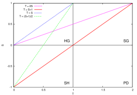
(a) Categorisation based on the game dynamics and the games.

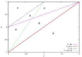
(b) Categorisation based on the game dynamics.

Figure 1: Game domains.

Understanding the evolution of cooperation among selfish agents is clearly an important and challenging task. Much effort has been put into achieving this using the PD game as a model [10]. When the population is mixed, where each player is equally likely to meet any other, natural selection favours defection over cooperation [9]. Hence, Nowak and May [10] studied the impact of arranging PD players in a two-dimensional array and concluded that cooperators and defectors can coexist indefinitely. Since then, considerable attention has been given to studying evolutionary game dynamics in spatial settings. In these settings, players are arranged as the vertices of a network and can play the game only with their immediate neighbours. The impact of network on the emergence of cooperation has also been emphasised in [5, 12, 16]. The way in which cooperation evolves in spatial settings is called network reciprocity [9], where cooperators survive by forming a cluster and helping each other within the cluster so that the defectors at the border cannot fare any better. In this paper we consider two extreme cases of the spatial setting. First, we consider the cycle graph in which the impact of the topology on the evolution is strongest [11]. Second, we consider the complete graph which models a mixed population. Several previous studies have focused on these types of graphs (see, for example, [1, 5, 11, 15]).

In evolutionary game theory, the payoffs are regarded as the Darwinian fitness [11]. During the evolution, strategies earning higher payoffs become more common in the population. Inheritance and imitation are two mechanisms by which successful strategies may spread. Between the two, imitation gives the more practical dynamics [3, p. 86]. Many versions of imitation have been studied in this context. Nowak and May [10] studied the imitation rule known as unconditional-imitation or imitate-the-best. Here, each player imitates the neighbour earning the highest payoff among the immediate neighbours and himself, in each round of the game. Furthermore, one of the three update rules studied in [11] is the asynchronous version of the proportional-imitation [3, p. 87] rule. Under this rule, in each round of the game, a random individual is given a chance to update his strategy. The individual then chooses a neighbour uniformly at random and imitates the neighbour with some probability proportional to the payoff difference. (A simpler version of this update rule is called imitate the better [3, p. 87], in which an updating individual always imitates the randomly selected neighbour, but only if the neighbour’s payoff is higher.) The synchronous version of this has been studied in [14, 15]. In this rule, each individual updates his strategy at the end of each round of the game in this fashion. ([14] refers to this as the replicator rule.) Finally, a stochastic combination of both versions of the proportional-imitation rule has been studied in [13]. Among the variations of imitation update rule, proportional-imitation rules perform optimally, both from the individual’s perspective and from the perspective of the population as a whole [17]. In this paper, we will study the synchronous version of the proportional-imitation rule. In the rest of this paper, we frequently refer to this rule just as the imitation update rule.

Most of the previous work on imitation rules has been empirical. For instance, the imitate-the-best rule on a two dimensional grid was studied in [10] using simulations; the synchronous proportional-imitation rule on different types of graphs was explored in [14, 15] using simulations; and both of these imitation rules were investigated in [13] using simulations. The reason for the lack of rigorous analysis is that a vast number of possible patterns of strategies can be generated [9]. The empirical results give insights into the evolution, but some of the results cannot properly be understood without theoretical underpinning. On the theoretical side, the asynchronous version of the proportional-imitation-rule on the cycle was analysed in [11] using fixation probabilities. The fixation probability is the probability that a population adopting the same strategy is overrun by a single individual adopting a mutant strategy. Although the results presented in [11] are interesting, the analysis based on fixation probabilities has two weaknesses. First, it does not show what happens when mutants invade in pairs, triples, etc. Second, it does not reveal any information about the rate of convergence to cooperation.

Here we will study the synchronous proportional-imitation rule on cycles and complete graphs rigorously. Similar rigorous results were given for the Pavlov or Highest Cumulative Reward rule in the Iterated PD game (see [1, 8] for details). Here, we make no assumptions about the initial configuration. We then calculate the time it takes for a steady state to be reached in these settings. By doing so, we provide rigorous support for the experimental results observed by [15] in complete graphs. In addition, we do a similar study for the cycle. Interestingly, this simple type of graph gives evidence that there are graphs on which cooperators and defectors cannot coexist for any of the four games, except for some specific payoffs values (i.e. $T=S+1$ and $T=(S+1)/2$). Furthermore we provide supporting simulation results for both types of graph.

The outline of this paper is as follows: Some preliminaries are described in Section 2. Section 3 investigates the dynamics of the imitation on the cycle, while Section 4 investigates the same on the complete graph. Empirical results appear in Section 5. The impact of our results is discussed in Section 6. Finally, concluding remarks are presented in Section 7.

2 Preliminaries

Let $G=(V,E)$ be a connected graph with vertices $V=\{v_{i}:i=0,1,\ldots,n-1\}.$ Each player at the vertex $i$ $(0\leq i\leq n-1)$ has a state $\mathcal{S}_{i}\in\{0,1\}$, where $0$ represents defection and $1$ represents cooperation. In addition, $\star$ is used as the don’t care symbol for the states when the particular value of the state does not matter in the discussion (e.g.  $0\star 1000$).

We will now define formally the proportional-imitation rule [3] with synchronous update. According to this rule, in each generation, each vertex $v_{i}$ ($0\leq i<n$) plays the game with all its $\mathcal{N}_{i}$ neighbours, and stores the accrued payoff for that generation as $P_{i}$. At the end of the generation, all vertices simultaneously update their strategies as follows: each vertex $v_{i}$ chooses one of its neighbours u.a.r. (say $v_{j}$) and copies the strategy of $v_{j}$ with probability

$$p_{i}=\max\left\{0,\dfrac{P_{j}-P_{i}}{m\alpha}\right\},$$

where $\alpha=\max\{T,1\}-\min\{S,0\}$, and $m=\max\{\mathcal{N}_{i},\,\mathcal{N}_{j}\}$. The denominator $m\alpha$ is a scaling factor which ensures that $p_{i}\in[0,1]$. Here, $p_{i}$ is called the switching probability of $v_{i}$. Note that if $P_{i}\geq P_{j}$, $v_{i}$ keeps the same strategy, i.e. the switching probability $p_{i}=0$. Clearly, the value of $m$ is 2 for cycles and $n-1$ for complete graphs.

We are interested to find the absorption time which is defined as the time required for the system to reach a steady state. The absorption time is determined in terms of the number of generations it takes for absorption as a function of the number of players, $n$. All-cooperate (where all players cooperate) and all-defect (where all players defect) are clearly two steady states under the imitation update rule. And there may exist other steady state configurations, where cooperators and defectors can coexist. Once the system reaches any of these states, it will remain there forever.

3 Imitation on the cycle

Suppose that a minimum of three agents occupy the vertices of a cycle graph $G=(V,E)$, where

$$V=\{v_{i}:i=0,1,\ldots,n-1\}\ \ \textrm{and}\ \ E=\{\{v_{i},v_{i+1}\}:i=0,1,\ldots,n-1\}\ .$$

Here and throughout this paper, addition and subtraction on the vertex subscripts is performed modulo $n$. We now introduce some terminology. Let $\mathcal{S}\in\{0,1\}^{V}$ be given. A cooperator-run (resp. defector-run) in $\mathcal{S}$ is an interval $[i,j]$ where $0\leq i,j<n$, such that $S_{k}=1$ (resp. $0$) for $i\leq k\leq j$ and $\mathcal{S}_{i-1}=0$ (resp. 1), $\mathcal{S}_{j+1}=0$ (resp. 1). We use c-run to denote the cooperator-run and d-run to denote the defector-run. It is possible to have $j\leq i$, since we are working modulo $n$. Clearly all runs are disjoint.

Suppose that $\mathcal{R}_{\textrm{d}}=[i,j]$ is a d-run where the subscript d stands for defectors. The length of the run $\mathcal{R}_{\textrm{d}}$, denoted by $\ell(\mathcal{R}_{\textrm{d}})$, is the number of defectors in the run, i.e. $\ell(R_{\textrm{d}})=j-i+1\mod n$. We will refer to a d-run of length $\ell$ as an $\ell_{\textrm{d}}$-run. A $1_{\textrm{d}}$-run will also be called a singleton defector and a $2_{\textrm{d}}$-run will also be called a pair of defectors. There are two outer rim edges associated with $\mathcal{R}_{\textrm{d}}$, namely $\{i-1,i\}$ and $\{j,j+1\}$. We use similar notations for c-runs, but with subscript c, which stands for cooperators. For example, $\ell_{\textrm{c}}$-run represents a c-run of length $\ell$. A run, c-run or d-run, is said to grow if its length increases. A run whose length cannot be reduced to zero through any combination of updates is called a barrier. A run is said to be deleted if all its vertices change from defector to cooperator or vice versa.

The main results for the game on cycle are listed below. The proofs are presented in the subsequent sections.

Initial configuration:  We assume that the initial configuration for the game is random: each vertex on the cycle is independently assigned as a cooperator with constant probability $p_{\textrm{c}}$ and as a defector with probability $1-p_{\textrm{c}}$ at the beginning of the game. Then, the following theorems give the absorption time for the $n$-vertex cycle.

Theorem 1.

If the payoffs are such that $S+1<T$, then the game converges to the all-defect state in time $O(n)$ with high probability.

Theorem 2.

If the payoffs satisfy

Case I:

$\tfrac{S+1}{2}<T<S+1$ and $T>2S,$ or

Case II:

$\tfrac{S+1}{2}<T<2S$,

then the game converges to the all-cooperate state in time $O(n)$ with high probability.

Theorem 3.

If the payoffs satisfy

Case I:

$0<T<\tfrac{S+1}{2}$ and $T>2S$, or $S<T<2S$ and $T<\tfrac{S+1}{2}$, or

Case II:

$T<S$,

then the game converges to the all-cooperate state in time $O(\log n)$ with high probability.

Remark 1.

In this paper, an event $Y_{n}$ which depends on the size of the graph $n$ is said to happen with high probability, or in short w.h.p., if $\Pr(Y_{n})\to 1$ as $n\to\infty$.

3.1 Analysis

Suppose, without loss of generality, that the random neighbour chosen by $v_{i}$ for imitation is $v_{i+1}$. Then, the switching probabilities of $v_{i}$ for different values of $\mathcal{S}_{i}$ and $\mathcal{S}_{i+1}$ are given in Figure 2. Clearly, we can ignore the two cases where the updating vertex and the randomly chosen neighbour already follow the same strategy, hence imitation has no effect. Ignoring these cases and expanding the formulae in Figure 2 with the possible values of $\mathcal{S}_{i-1}$ and $\mathcal{S}_{i+2}$, we obtain the results in Figure 3. This figure also shows the variable names we use to denote these different probabilities. Now, it is obvious that the switching probability of $v_{i}$, when it randomly chooses $v_{i+1}$ for imitation, depends on the states $\mathcal{S}_{i-1},\mathcal{S}_{i},\mathcal{S}_{i+1}$, and $\mathcal{S}_{i+2}$. For notational convenience we write these states as $\mathcal{S}_{i-1}[\mathcal{S}_{i}]\mathcal{S}_{i+1}\mathcal{S}_{i+2}$ (e.g.  $0[1]11$), enclosing the state of $v_{i}$ in square brackets.

$\mathcal{S}_{i}$	$\mathcal{S}_{i+1}$	$p_{i}=\tfrac{P_{i+1}-P_{i}\rule{0.0pt}{7.83612pt}}{2\alpha}$
0	0	$\tfrac{(\mathcal{S}_{i+2}-\mathcal{S}_{i-1})T\rule{0.0pt}{7.83612pt}}{2\alpha}$
0	1	$\tfrac{(2S-T)+\mathcal{S}_{i+2}(1-S)-\mathcal{S}_{i-1}T\rule{0.0pt}{7.83612pt}}{2\alpha}$
1	0	$\tfrac{(T-2S)+\mathcal{S}_{i+2}T-\mathcal{S}_{i-1}(1-S)\rule{0.0pt}{7.83612pt}}{2\alpha\rule[-3.61664pt]{0.0pt}{0.0pt}}$
1	1	$\tfrac{(\mathcal{S}_{i+2}-\mathcal{S}_{i-1})(1-S)\rule{0.0pt}{7.83612pt}}{2\alpha\rule[-3.61664pt]{0.0pt}{0.0pt}}$

Figure 2: Switching probabilities for $v_{i}$, provided $v_{i+1}$ has been chosen by $v_{i}$ for imitation.

Note that the prerequisite for a player to switch strategy through imitation is to have at least one neighbour with a different strategy. Hence, the strategy changes on the cycle can happen only at the vertices of the outer rim edges of a c-run or a d-run, since all other vertices incident on a run have both their neighbours employing the same strategy as theirs. So, it is sufficient to focus our analysis on the borders of runs.

$\mathcal{S}_{i}$	$\mathcal{S}_{i+1}$	$\mathcal{S}_{i-1}\mathcal{S}_{i+2}$
		00	01	10	11
0	1	$a=\tfrac{2S-T\rule{0.0pt}{7.83612pt}}{2\alpha}$	$b=\tfrac{S+1-T}{2\alpha}$	$c=\tfrac{2(S-T)}{2\alpha}$	$d=\tfrac{S+1-2T}{2\alpha}$
1	0	$\bar{a}=\tfrac{T-2S\rule{0.0pt}{7.83612pt}}{2\alpha\rule[-3.61664pt]{0.0pt}{0.0pt}}$	$\bar{c}=\tfrac{2(T-S)}{2\alpha}$	$\bar{b}=\tfrac{T-S-1}{2\alpha}$	$\bar{d}=\tfrac{2T-S-1}{2\alpha}$

Figure 3: Switching probabilities for $v_{i}$ for different possible neighbour-states.

For the analysis, we first need to know whether the values for the $p_{i}$’s are zero or not. As mentioned earlier, each game corresponds to a quadrant in the $ST$ plane as shown in Figure 1(a). Yet, we will not use this game-based categorisation in our analysis. This is because, although these games have different ($\alpha,S,T$) values, they share the same behaviour in some cases, as a result of having the same sign for $P_{i}-P_{j}$ :

• $T>\tfrac{S+1}{2}$ for PD and SG

• $T>2S$ for PD and SH

• $T>S$ for PD, SH and SG

Instead, we categorise the game domain into six regions based on the dynamics for the purpose of analysis, as shown in Figure 1(b) with labels A, B, C, D, E and F. Each of these regions is characterised by its boundary conditions. They are:

• Region A : $T>S+1$

• Region B : $\tfrac{S+1}{2}<T<S+1$ and $T>2S$

• Region C : $\tfrac{S+1}{2}<T<2S$

• Region D : $2S<T<\tfrac{S+1}{2}$

• Region E : $S<T<2S$ and $T<\tfrac{S+1}{2}$

• Region F : $T<S$

Next we prove a lemma that will be used frequently in the proofs.

Lemma 1.

Let $\ell_{t}$ be the length of a d-run at time $t$. If the length of the run reduces by at least $p$ in expectation for some constant $p>0$, the probability that the run is not deleted in $\tfrac{\ell_{0}}{p(1-\varepsilon)}$ generations is at most $e^{-\tfrac{\varepsilon^{2}\ell_{0}}{2(1-\varepsilon)}}$ for any $\varepsilon>0$.

Proof.

Let $\mathcal{T}$ be the time at which $\ell_{t}$ becomes $0$ for the first time. Let $X_{t}$ be the decrement of the length of the run at time $t$. Thus

$$X_{t}=\begin{cases}0&\text{if $\ell_{t}=0,$}\\ 1&\text{otherwise.}\end{cases}$$

Thus, for $t\leq\mathcal{T}$, the decrements are independent random variables with expectation $\mathbf{E}[X_{t}]\geq p$ where $X_{t}\in\{0,1\}$. Thus

$$\ell_{t}=\ell_{0}-\sum_{i=1}^{t}X_{i}\ .$$

For any $t\leq\mathcal{T}$, using the Chernoff bound, we get

$$\Pr\Bigg{(}\sum_{i=1}^{t}X_{i}\leq pt(1-\varepsilon)\Bigg{)}\leq\exp(-\tfrac{1}{2}\varepsilon^{2}pt),$$ (1)

for any $\varepsilon>0$. Since $\ell_{\mathcal{T}}=0$, we have

$$\sum_{i=1}^{\mathcal{T}}X_{i}\geq\ell_{0}\ .$$

Hence, applying (1) for $\mathcal{T}$ steps, we get

$$\Pr\bigg{(}\mathcal{T}\geq\dfrac{\ell_{0}}{p(1-\varepsilon)}\bigg{)}\leq\exp(-\tfrac{1}{2}\varepsilon^{2}p\mathcal{T})\leq\exp\left(-\tfrac{1}{2}\varepsilon^{2}p\tfrac{\ell_{0}}{p(1-\varepsilon)}\right)=\exp\left(-\tfrac{\varepsilon^{2}\ell_{0}}{2(1-\varepsilon)}\right)\ .$$

∎

Next we explore some properties of the initial random configuration.

3.1.1 Properties of the initial configuration

In this study, the initial configuration is assumed to be generated randomly as follows: each vertex on the cycle is independently assigned as a cooperator with constant probability $p_{\textrm{c}}$ and as a defector with probability $p_{\textrm{d}}=1-p_{\textrm{c}}$ at the beginning of the game. Hence, at the beginning of the game, the expected number of cooperators present on the cycle is $np_{\textrm{c}}$. So, it is reasonable to assume $p_{\textrm{c}}=\Omega(1/n)$, so that there will be some cooperators at the start.

Lemma 2.

The probability that there is no $k_{c}$-run, where $k\geq 1$ is a constant, on the cycle at the beginning of the game is at most $e^{-p_{\textrm{c}}^{k}\lfloor n/k\rfloor}$.

Proof.

Let $P_{k}$ be the probability that $k$-consecutive vertices are not all cooperators. Hence

$$P_{k}=(1-p_{\textrm{c}}^{k})\ .$$

There are $\lfloor n/k\rfloor$ disjoint $k$-segments on the cycle. As each vertex is assigned the initial state independently, these segments are independent. Hence, the probability that none of those segments is all-cooperators is

$$P_{k}^{\lfloor n/k\rfloor}=(1-p_{\textrm{c}}^{k})^{\lfloor n/k\rfloor}\leq e^{-p_{\textrm{c}}^{k}\lfloor n/k\rfloor},$$

and the lemma is proved. ∎

Lemma 3.

The following statement holds with high probability. The longest c-run generated in the initial configuration is of length $\lambda\log n$ for any $\lambda>0$ such that $\lambda\log(1/p_{\textrm{c}})>1$.

Proof.

Let $r_{\ell}$ be the number of c-runs of length $\ell$. So,

$$\mathbf{E}[r_{\ell}]=n{p_{\textrm{c}}}^{\ell}\ .$$

If $\ell=\lambda\log n$, then

$$\mathbf{E}[r_{\ell}]\ =\ n{p_{\textrm{c}}}^{\ell}\ =\ n{p_{\textrm{c}}}^{\lambda\log n}\ =\ n^{1-\lambda\log(1/p_{\textrm{c}})}\ .$$

So,

$$\Pr(r_{\ell}\neq 0)\leq n^{1-\lambda\log(1/p_{\textrm{c}})}\ .$$

Since $n^{1-\lambda\log(1/p_{\textrm{c}})}\to 0$ as $n\to\infty\,$ for $\lambda\log(1/p_{\textrm{c}})>1$, we do not expect to see any runs of length $\lambda\log n$ or longer and the lemma is proved. ∎

Lemma 4.

The following statement holds with high probability. The longest d-run generated in the initial configuration is of length $\lambda\log n$ for any $\lambda>0$ such that $\lambda\log(1/p_{\textrm{d}})>1$.

Proof.

The proof is entirely similar to that of Lemma 3, so will be omitted. ∎

Lemma 5.

Consider a segment on the cycle having d-runs of any length separated by $1_{c}$-runs. Such a segment must have a c-run of length greater than 1 at each end. Now, the following statement about this segment holds with high probability. The length of the longest such segment in the initial configuration is $O(\log n)$.

Proof.

The length of the segment can be calculated using a simple random walk. Suppose the vertices are assigned as cooperators (or ones) or defectors (or zeroes) from $v_{0}$ to $v_{n-1}$. At any time $t$, there can be four combinations of present and future assignments. They are: 00, 01, 10, and 11. Consider these as four states of a Markov chain $\mathcal{M}$, and denote these states by $s_{0},s_{1},s_{2},$ and $s_{3}$ respectively. The transition probabilities for these states are shown in Figure 4.

Figure 4: A random walk representing the generation of initial configuration, modelled as a four-state Markov chain. The edges of the state diagram are labelled with transition probabilities.

We are interested to find the total length of the d-runs connected by $1_{\textrm{c}}$-runs. Thus, we need to find the time to return to $s_{3}$, or equivalently, the time to go from $s_{2}$ to $s_{3}$. This time is exactly the length of the d-runs separated by singleton cooperators.

Clearly, from any other states of $\mathcal{M}$, there is a probability at least $p_{c}^{2}$ of reaching $s_{3}$ in two steps. Hence the probability that $s_{3}$ will not be reached in $2t$ steps is at most $p_{c}^{2t}$. Thus the probability that there exists any such run of length $\lambda\log n$, for any $\lambda>0$, is at most

$$np_{\textrm{c}}^{\lambda\log n}<\frac{1}{n},\mbox{ if }\ \ \lambda>\dfrac{2}{\log(1/p_{\textrm{c}})}\ .$$

Hence, if $\lambda>\tfrac{2}{\log(1/p_{\textrm{c}})}$, the probability of finding this special configuration of length $\lambda\log n$ tends to 0 as $n\to\infty.$ Thus, with high probability, the maximum length of the segment is $O(\log n)$. ∎

Lemma 6.

The following statement holds with high probability. The longest sequence of alternating 1’s and 0’s in the initial configuration is at most $2\lambda\log n$, for any $\lambda>0$ such that $\lambda\big{(}\log(1/p_{\textrm{c}})+\log(1/p_{\textrm{d}})\big{)}>1$.

Proof.

Let $r_{\ell}$ be the number of occurrences of a chain of length $\ell$ having alternating 1’s and 0’s. Suppose $\ell$ is even, without loss of generality. Then we have

$$\mathbf{E}[r_{\ell}]=n{p_{\textrm{c}}}^{\tfrac{\ell}{2}}{p_{\textrm{d}}}^{\tfrac{\ell}{2}}\ .$$

If $\ell=2\lambda\log n$, then

$$\mathbf{E}[r_{\ell}]\ =\ n{p_{\textrm{c}}}^{\lambda\log n}{p_{\textrm{d}}}^{\lambda\log n}\ =\ n^{1-\lambda\log(1/p_{\textrm{c}})-\lambda\log(1/p_{\textrm{d}})}\ .$$

So, if $\lambda\big{(}\log(1/p_{\textrm{c}})+\log(1/p_{\textrm{d}})\big{)}>1$, we have

$$\Pr(r_{\ell}\neq 0)\leq\ n^{1-\lambda\log(1/p_{\textrm{c}})-\lambda\log(1/p_{\textrm{d}})}\to 0\mbox{ as }n\to\infty.\qed$$

3.1.2 Emergence of defection

In this section we prove that the defection emerges fast for the games in the region labelled A in Figure 1(b). This region, having $S+1<T$, covers the whole PD domain and half the domain of SH and SG. The table below shows which of the switching probabilities are zero for the vertex $v_{i}$.

$\mathcal{S}_{i}$	$\mathcal{S}_{i+1}$	$\mathcal{S}_{i-1}\mathcal{S}_{i+2}$
		00	01	10	11
$0$	$1$	$0$	$0$	$0$	$0$
$1$	$0$	$+$	$+$	$+$	$+$

Here, no defector will ever become a cooperator, but cooperators can become defectors. So, the game converges to the all-defect state fast. The following lemmas prove this.

Lemma 7.

Suppose $\mathcal{R}_{\textrm{c}}$ is the longest c-run in the cycle when the game is started and let $\ell(\mathcal{R}_{\textrm{c}})=\gamma$. Provided $S+1<T$, probability that all-defect state is not reached in $\frac{\gamma}{\bar{b}(1-\varepsilon)}$ generations is at most $e^{-\tfrac{\varepsilon^{2}\gamma}{2(1-\varepsilon)}}$, for any $\varepsilon>0$.

Proof.

In synchronous updating, each vertex updates its strategy at the end of every generation. When $S+1<T$, the only vertices that imitate their neighbours are the cooperators at either end of a c-run. (Note that a $1_{c}$-run has only one such cooperator.) A cooperator at this position chooses a defector for imitation with probability $\tfrac{1}{2}$. Let $p$ be defined to be the minimum of the four possible switching probabilities (see Figure 3). It can be easily verified that we have

$$p=\min\{\bar{a},\bar{b},\bar{c},\bar{d}\}=\bar{b}\ .$$

Then, an $\ell_{\textrm{c}}$-run $(2\leq\ell<n)$ reduces in length at either end with probability at least $\tfrac{1}{2}p$ and a $1_{c}$-run is deleted with probability at least $p$, in every generation. Thus, the expected decrease in the length of any c-run is at least $\bar{b}$. The time it takes for the longest c-run to be deleted completely is precisely the absorption time, since shorter runs are deleted faster. The result then follows from Lemma 1. ∎

In the worst case, the length of the longest c-run ($\gamma$) can be $n$. This means all players cooperate at the beginning, which is an absorbing state. Hence, the all-defect state is never reached. But, if $\gamma=n-1$, in view of Lemma 7, it takes $\tfrac{(n-1)}{\bar{b}(1-\varepsilon)}\approx\tfrac{n}{\bar{b}}$ generations for the convergence to defection. However, it was shown in Lemma 4 that, when $p_{\textrm{c}}<1$, the length of the longest c-run is $O(\log n)$. Theorem 1 combines all these results.

Proof of Theorem  1: By Lemma 4, the longest c-run present on the cycle at the beginning of the game is of length $\lambda\log n$ w.h.p for any $\lambda>0$ such that $\lambda\log(1/p_{\textrm{c}})>1$. Then, by Lemma 7, the probability that the steady state has not been reached in

$$\dfrac{\lambda\log n}{\bar{b}(1-\varepsilon)}=O(\log n)$$

generations is at most $n^{-\tfrac{\varepsilon^{2}\lambda}{2(1-\varepsilon)}}$ for any $\varepsilon>0$, where $\bar{b}=\tfrac{T-S-1}{2\alpha}\$ and $\alpha=\max\{T,1\}-\min\{S,0\}$. For a suitable value for $\lambda$, this probability tends to 0 as $n\to\infty$ which completes the proof. $\Box$

3.1.3 Emergence of cooperation

In this section, we prove that cooperation emerges fast in regions B, C, D, E, and F. Before analysing these, let us first look at some common characteristics shown by the regions B, C, D and E. Figure 5 shows which of the switching probabilities are zero for each of these regions. Note, from Figure 1(b), that the regions B, C, D and E satisfy $T<S+1$. Hence, Lemma 8 holds for these regions.

$\mathcal{S}_{i}$	$\mathcal{S}_{i+1}$	$\mathcal{S}_{i-1}\mathcal{S}_{i+2}$
		00	01	10	11
$0$	$1$	$0$	$+$	$0$	$0$
$1$	$0$	$+$	$+$	$0$	$+$

(a) Region B

$\mathcal{S}_{i}$	$\mathcal{S}_{i+1}$	$\mathcal{S}_{i-1}\mathcal{S}_{i+2}$
		00	01	10	11
$0$	$1$	$+$	$+$	$0$	$0$
$1$	$0$	$0$	$+$	$0$	$+$

(b) Region C

$\mathcal{S}_{i}$	$\mathcal{S}_{i+1}$	$\mathcal{S}_{i-1}\mathcal{S}_{i+2}$
		00	01	10	11
$0$	$1$	$0$	$+$	$0$	$+$
$1$	$0$	$+$	$+$	$0$	$0$

(c) Region D

$\mathcal{S}_{i}$	$\mathcal{S}_{i+1}$	$\mathcal{S}_{i-1}\mathcal{S}_{i+2}$
		00	01	10	11
$0$	$1$	$+$	$+$	$0$	$+$
$1$	$0$	$0$	$+$	$0$	$0$

(d) Region E

Figure 5: Switching probabilities for B, C, D and E.

Lemma 8.

In B, C, D and E, if a c-run $\mathcal{R}_{\textrm{c}}$ of length at least $2$ is adjacent to d-runs of length at least $2$ at each end, the c-run grows in length or remains as it is. The expected growth of the run in one generation is $b$.

Proof.

The proof is based on the observation that the switching probability is positive for $0[0]11$ and zero for $1[1]00$ in the regions in question.

Now, suppose $\mathcal{R}_{\textrm{c}}=[i,j]$ such that $\ell(\mathcal{R}_{\textrm{c}})\geq 2$. Suppose $\mathcal{R}_{\textrm{c}}$ is bordered by at least two defectors on both sides, so we have $\star 001100\star$. The vertices of the outer-rim edges of $R_{\textrm{c}}$, namely $v_{i-1},v_{i},v_{j}$ and $v_{j+1}$, are in states $0,1,1$ and $0$ respectively. Possible changes to these vertices after a generation are:

• $v_{i-1}$, which is a defector itself, has another defector on its left and a cooperator on its right. Hence, switching can happen only if $v_{i-1}$ tries to imitate from its right. As Figure 3 indicates, this happens with probability $\tfrac{1}{2}b$ (as the right neighbour is chosen with probability $\tfrac{1}{2}$ and the actual switching happens independently with probability $b$ which is non-zero according to Figure 5). This makes $\mathcal{R}_{\textrm{c}}$ longer in length by $1$.

• $v_{i}$, which is a cooperator itself, has another cooperator on its right and a defector on its left. Hence an effective imitation can happen only when it copies from its left neighbour. But, as shown in Figure 5, the probability of switching to defection in this scenario (i.e. $1[1]00$) is zero. Hence, this vertex will not change its strategy.

• By symmetry, $v_{j}$ does the same as $v_{i}$.

• By symmetry, $v_{j+1}$ does the same as $v_{i-1}$.

Hence, $\mathcal{R}_{\textrm{c}}$ grows in length with some non-zero probability. The expected growth of $\mathcal{R}_{\textrm{c}}$ at either end is $\tfrac{1}{2}b$ in one generation. Hence the total expected growth of the run equals $b$. ∎

Remark 2.

Lemma 8 implies that an $\ell_{\textrm{c}}$-run ($\ell\geq 2$) bordered by at least 2 defectors is hard to eliminate in B, C, D and E. We say “hard” because, as we will see later, one such configuration can be eliminated by another in some regions. By combining this observation with the dynamics of each region separately, we later establish the conditions determining a barrier for each region.

Now we investigate the dynamics of a singleton cooperator having at least two defectors at its either end.

Lemma 9.

A singleton cooperator ($1_{\textrm{c}}$-run) bordered on both sides by at least two defectors (i.e. $\star 00100\star$) can grow up to length 3 in C and E, whereas it is deleted in B and D.

Proof.

Let $R_{\textrm{c}}=[i,i]$ be a $1_{\textrm{c}}$-run and let $\mathcal{S}_{i-2}=\mathcal{S}_{i-1}=\mathcal{S}_{i+1}=\mathcal{S}_{i+2}=0$. Here, $v_{i}$ might imitate both its neighbours and has $0[1]00$ in both cases. As the comparison tables in Figure 6 show, the switching probability for $0[1]00$ is positive in B and D, and zero in E and C. Hence, $v_{i}$ might become a defector in B and D, but will remain as a cooperator in E and C.

$\mathcal{S}_{i}$	$\mathcal{S}_{i+1}$	$\mathcal{S}_{i-1}\mathcal{S}_{i+2}$
		00
$0$	$1$	$0$
$1$	$0$	$+$

(a) B and D

$\mathcal{S}_{i}$	$\mathcal{S}_{i+1}$	$\mathcal{S}_{i-1}\mathcal{S}_{i+2}$
		00
$0$	$1$	$+$
$1$	$0$	$0$

(b) C and E

Figure 6: The switching probabilities related to singleton cooperators

Next, let us see what happens to the neighbours of $R_{\textrm{c}}$, namely $v_{i-1}$ and $v_{i+1}$. It can be easily verified that both $v_{i-1}$ and $v_{i+1}$ have a defector at one side and the cooperator $v_{i}$ at the other side. So, the switching can happen only when these vertices copy from $v_{i}$. In that case, the defectors appear as $0[0]10$ which has a zero switching probability in B and D and a non-zero switching probability in C and E.

To sum up, in B and D, while $v_{i}$ switches to defection, its defector neighbours remain unchanged, hence $R_{\textrm{c}}$ is deleted. But, in C and E, while $v_{i}$ remains as a cooperator, its neighbours can become cooperators too, potentially increasing the length of the $1_{c}$-run up to 3. ∎

A singleton defector having longer c-run neighbours has the potential to grow in regions B and C, as the following lemma shows.

Lemma 10.

A singleton defector ($1_{\textrm{d}}$-run) bordered on both sides by at least two cooperators (i.e. $\star 11011\star$) can grow up to length 3 in B and C, whereas it is deleted in D and E.

Proof.

In this case, the defector in the middle could imitate from both its neighbours and has the neighbourhood of $1[0]11$ on either side, and the adjacent cooperators can copy only from the middle defector and have $1[1]01$. The dynamics for these two cases are compared in Figure 7.

$\mathcal{S}_{i}$	$\mathcal{S}_{i+1}$	$\mathcal{S}_{i-1}\mathcal{S}_{i+2}$
		11
$0$	$1$	$0$
$1$	$0$	$+$

(a) B and C

$\mathcal{S}_{i}$	$\mathcal{S}_{i+1}$	$\mathcal{S}_{i-1}\mathcal{S}_{i+2}$
		11
$0$	$1$	$+$
$1$	$0$	$0$

(b) E and D

Figure 7: The switching probabilities related to singleton defectors

As Figure 7 shows, in E and D, the switching probability is positive for $1[0]11$ and zero for $1[1]01$. Consequently, in $\star 11011\star$, the defector might become a cooperator while its neigbouring cooperators remain unchanged. Hence, the $1_{d}$-run is deleted in E and D. But, in the case of B and C, the opposite is true: the middle defector will remain as it is while its cooperator neighbours switch to defection. Thus, the singleton defector might become a $2_{\textrm{d}}$-run or a $3_{\textrm{d}}$-run as claimed. ∎

Let us now analyse each region separately.

Region B ($\tfrac{S+1}{2}<T<S+1$ and $T>2S$)

Figure 1(b) shows this region with label B. Figure 5(a) shows which cases have zero and non-zero switching probabilities. In this section we prove that cooperation evolves in linear time in this region. Analysing the actual imitation process to prove this is complicated. Fortunately, we can use a simplified model for this purpose. The following lemma forms the basis for the simplification of the process.

Lemma 11.

An $\ell_{\textrm{c}}$-run ($\ell\geq 4$) is a barrier in region B, whereas a c-run shorter than 4 might be deleted through a sequence of updates.

Proof.

In region B,

a $1_{\textrm{c}}$-run is always deleted: 

Lemma 9 shows that a $1_{\textrm{c}}$-run is deleted if it has two defectors on both sides. Now, when a $1_{\textrm{c}}$-run is adjacent to a $1_{\textrm{d}}$-run on either side, as in $\star 10[1]01\star$, it is readily verified that the $1_{\textrm{c}}$-run will be turned into a defector whereas the adjacent defectors remain unchanged. Thus, a $1_{\textrm{c}}$-run cannot grow if it is adjacent to singleton defectors at both ends. Obviously this would be the case when a $1_{\textrm{c}}$-run has a singleton defector on one side and at least two defectors on the other side.

It is noteworthy that if all the cooperators on the cycle exist as $1_{\textrm{c}}$-runs, the game converges to all-defect, since singleton cooperators can never survive.

a $2_{\textrm{c}}$-run can grow or be deleted: 

A $2_{\textrm{c}}$-run grows if it is bordered by at least two defectors as shown in Lemma 8. Now, when a $2_{\textrm{c}}$-run is adjacent to $1_{\textrm{d}}$-runs on both sides, either of the $1_{\textrm{d}}$-runs can grow, deleting a cooperator in the $2_{\textrm{c}}$-run, as illustrated in Lemma 10, and removing the $2_{\textrm{c}}$-run completely. Thus, when a $2_{\textrm{c}}$-run is adjacent to a $1_{\textrm{d}}$-run on one side and at least two defectors on the other, it has the possibility of growing or reducing to a $1_{\textrm{c}}$-run which is subsequently deleted.

An interesting case shows that even a $2_{\textrm{c}}$ run bordered by at least two defectors can be removed if it is adjacent to another $2_{\textrm{c}}$-run. Consider the configuration $0011001100$. This might first become $0011101100$, then become $001100010$, and finally become $001100000$, deleting one of the $2_{\textrm{c}}$-runs completely.

a $3_{\textrm{c}}$-run can grow or be deleted: 

Like the pair of cooperators, although a $3_{\textrm{c}}$-run can grow when it is bordered by two defectors at either end, there is a possibility of it being deleted if it has singleton defectors at both ends.

an $\ell_{\textrm{c}}$-run ($\ell\geq 4$) can never be deleted: 

Even if there are singleton defectors at either end of a $4_{\textrm{c}}$-run , the run’s length will be reduced to 2 in the worst case. The resulting $2_{\textrm{c}}$-run will then be bordered by two defectors, hence will start growing again, as shown in Lemma 8. Obviously, longer runs are more stable and cannot be deleted.

In short, the key observations are: $1_{\textrm{c}}$-runs are always deleted; $2_{\textrm{c}}$-runs and $3_{\textrm{c}}$-runs might grow or be deleted; and, runs of length 4 or more can never be deleted. Hence a run of length 4 or more is a barrier. ∎

Clearly, the worst case for the evolution of cooperation is when there is only one minimal barrier (a $4_{\textrm{c}}$-run) at the start of the game. We use this worst case scenario to determine the absorption time. But, we need to address an issue before doing that. Although the time calculated in this way gives the worst case for a c-run to grow until the all-cooperate state is reached, it might not include the overhead time required if there are many runs. There are two types of such overheads: the time spent on handling short runs that can become a barrier or be deleted, and the time spent on merging two c-runs. We first calculate the worst case time for these overheads in Lemma 12 and 13 respectively.

Lemma 12.

Let $\phi_{s}$ denote the expected time it takes for a $1_{\textrm{c}},2_{\textrm{c}},3_{\textrm{c}}$-run to be deleted or become a barrier (a run of length 4). Then $\phi_{s}=O(1)$.

Proof.

Recall that a singleton cooperator can never grow. According to Figure 3, it is deleted with probability

• $\bar{a}$ if it is in the form $00[1]00$,

• $\bar{c}$ if it is in the form $10[1]01$, and

• $\tfrac{1}{2}(\bar{a}+\bar{c})$ if it is in the form $10[1]00$.

We also have $\bar{a}<\bar{c}$. Hence, the worst expected time it takes for a $1_{\textrm{c}}$ to be removed is $1/\bar{a}$, since it has the geometric distribution with probability of success of $\bar{a}$. Now it is enough to determine the time it takes for a $2_{\textrm{c}}$-run or a $3_{\textrm{c}}$-run to become a $1_{\textrm{c}}$-run or a $4_{\textrm{c}}$-run, as we know that $1_{\textrm{c}}$’s are removed in constant time. For calculating this, consider a random walk on the number of cooperators, i.e. {1,2,3,4}. Then we need to show that the walk reaches 1 or 4 in constant time irrespective of where it starts. Next we determine the corresponding probabilities of this process.

Suppose the current position of the random walk is 2 or 3, i.e. there is a $2_{\textrm{c}}$-run or a $3_{\textrm{c}}$-run respectively. A $2_{\textrm{c}}$-run or a $3_{\textrm{c}}$-run can exist in three forms:

• $001100$ or $0011100$. In this case, the probability of going to the right is $b-\tfrac{1}{4}b^{2}$ and the probability of going to the left is 0.

• $001101$ or $0011101$. In this case, the probability of going to the right is $\tfrac{1}{2}b\bigl{(}1-\tfrac{1}{2}\bar{d}\bigr{)}$ and the probability of going to the left is $\tfrac{1}{2}\bar{d}\bigl{(}1-\tfrac{1}{2}b\bigr{)}$.

• $101101$ or $1011101$. In this case, the probability of going to the right is $0$ and the probability of going to the left is $\bar{d}-\tfrac{1}{4}\bar{d}^{2}$.

We want an upper bound on the time it takes to reach state $1$ or $4$. It takes longest to reach $4$ if the probability of moving to the right is the minimum non-null probability, $r$ say. If the probability of moving to right is zero, the walk never reaches $4$ and is absorbed at $0$. We have

$$r=\min\bigl{\{}b-\tfrac{1}{4}b^{2},\tfrac{1}{2}b\bigr{(}1-\tfrac{1}{2}\bar{d}\bigl{)}\bigr{\}}\ .$$

Similarly, it takes longest to reach $1$ when the probability $q$ of moving left from $2$ or $3$ is

$$q=\min\bigl{\{}\bar{d}-\tfrac{1}{4}\bar{d}^{2},\tfrac{1}{2}\bar{d}\bigr{(}1-\tfrac{1}{2}b\bigl{)}\bigr{\}}\ .$$

So we have a Gambler’s Ruin problem with absorbing barriers at $1$ and $4$. Using the standard results when $r+q=1$ (see, for example, Feller[2, p. 345]), if the game is started from state $\ell\in\{2,3\}$, the expected duration of the process is

$$D_{\ell}=\begin{cases}\dfrac{\ell}{q-r}-\dfrac{4}{q-r}\dfrac{1-(q/r)^{\ell}}{1-(q/r)^{4}}&\text{if $r\neq q$,}\\ \ell(4-\ell)&\text{if $r=q.$}\end{cases}$$

Let $D_{\max}=\max\{D_{2},D_{3}\}$. Clearly $D_{max}$ is constant as it only involves the constants $q$ and $r$ which, in turn, can be expressed in terms of the constants $S$ and $T$. There is a self-loop at 2 and 3 with constant probability, at most $1-(r+q)$, but this slows down the random walk only by a constant factor. Thus it takes only constant time to reach $1$ or $4$. We showed earlier that it takes constant time to go from $1$ to $0$. Hence the total expected time is constant. ∎

The other overhead of having more than one run is the time required to merge them. Two barriers merge together when they are separated by two defectors and both defectors switch to cooperation simultaneously. As the switching of both defectors happens independently with some probability, there is a possibility that only one of the two defectors switches to cooperation whereby a singleton defector is created between the two c-runs. Then, as shown in Lemma 10, the singleton defector can grow up to length $3$. And then the barriers start growing again. This is repeated until the runs are merged. The following lemma proves that the worst case merging time for two c-runs of length at least 4 is a constant.

Lemma 13.

Let $\phi_{m}$ denote the expected time it takes for two barriers (i.e. two c-runs of length at least 4) separated by 1 or 2 defectors to merge together. Then $\phi_{m}=O(1)$.

Proof.

The merging process can be modelled as a simple absorbing Markov chain with states $M_{i}$ ($0\leq i\leq 3$) where $i$ denote the number of defectors in between the barriers. $M_{0}$ is the absorbing state and all other states are transient. Using Figure 3, we can determine the transition probabilities for this Markov chain. The corresponding transition matrix in canonical form is

$$\hbox{}\vbox{\kern 0.86108pt\hbox{$\kern 0.0pt\kern 2.5pt\kern-5.0pt\left[\kern 0.0pt\kern-2.5pt\kern-5.55557pt\vbox{\kern-0.86108pt\vbox{\vbox{ \halign{\kern\arraycolsep\hfil\@arstrut$\kbcolstyle#$\hfil\kern\arraycolsep& \kern\arraycolsep\hfil$\@kbrowstyle#$\ifkbalignright\relax\else\hfil\fi\kern\arraycolsep&& \kern\arraycolsep\hfil$\@kbrowstyle#$\ifkbalignright\relax\else\hfil\fi\kern\arraycolsep\cr 5.0pt\hfil\@arstrut$\scriptstyle$\hfil\kern 5.0pt&5.0pt\hfil$\scriptstyle M_{1}$\hfil\kern 5.0pt&5.0pt\hfil$\scriptstyle M_{2}$\hfil\kern 5.0pt&5.0pt\hfil$\scriptstyle M_{3}$\hfil\kern 5.0pt&5.0pt\hfil$\scriptstyle M_{0}\\M_{1}$\hfil\kern 5.0pt&5.0pt\hfil$\scriptstyle(1-\bar{d}/2)^{2}$\hfil\kern 5.0pt&5.0pt\hfil$\scriptstyle\bar{d}(1-\bar{d}/2)$\hfil\kern 5.0pt&5.0pt\hfil$\scriptstyle\bar{d}^{2}/4$\hfil\kern 5.0pt&5.0pt\hfil$\scriptstyle 0\\M_{2}$\hfil\kern 5.0pt&5.0pt\hfil$\scriptstyle b(1-b/2)$\hfil\kern 5.0pt&5.0pt\hfil$\scriptstyle(1-b/2)^{2}$\hfil\kern 5.0pt&5.0pt\hfil$\scriptstyle 0$\hfil\kern 5.0pt&5.0pt\hfil$\scriptstyle b^{2}/4\\M_{3}$\hfil\kern 5.0pt&5.0pt\hfil$\scriptstyle b^{2}/4$\hfil\kern 5.0pt&5.0pt\hfil$\scriptstyle b(1-b/2)$\hfil\kern 5.0pt&5.0pt\hfil$\scriptstyle(1-b/2)^{2}$\hfil\kern 5.0pt&5.0pt\hfil$\scriptstyle 0\\M_{0}$\hfil\kern 5.0pt&5.0pt\hfil$\scriptstyle 0$\hfil\kern 5.0pt&5.0pt\hfil$\scriptstyle 0$\hfil\kern 5.0pt&5.0pt\hfil$\scriptstyle 0$\hfil\kern 5.0pt&5.0pt\hfil$\scriptstyle 1$\hfil\kern 5.0pt\crcr}}}}\right]$}}\ .$$

Note that all transition probabilities are constants. Hence, using standard methods, absorption time can be calculated. Let $\tau_{i}$ be the absorption time when the chain starts at $M_{i}$. Then we get

$$\begin{bmatrix}\tau_{1}\\ \tau_{2}\\ \tau_{3}\end{bmatrix}=\begin{bmatrix}\dfrac{16b-8{b}^{2}+{b}^{3}+16\bar{d}-4b\bar{d}-b{\bar{d}}^{2}}{\bar{d}{b}^{2}(4-b-\bar{d})}\ \\[2.15277pt] \dfrac{2(8b-6b^{2}+b^{3}+8\bar{d}-2b\bar{d}-bd^{2})}{\bar{d}b^{2}(4-b-\bar{d})}\ \\[2.15277pt] \dfrac{16b-12b^{2}+3b^{3}+16\bar{d}-3b\bar{d}^{2}}{\bar{d}b^{2}(4-b-\bar{d})}\end{bmatrix}\ .$$

The worst case merging time $\phi_{m}=\max\{\tau_{1},\tau_{2},\tau_{3}\}$. Since the time calculation involves only constants, $\phi_{m}$ is constant, and the lemma is proved. ∎

Now we will assume that when the game is started there is a $4_{\textrm{c}}$-run and an $(n-4)_{\textrm{d}}$-run on the cycle. The following lemma proves that it takes linear time for the $4_{\textrm{c}}$-run to grow up to length $n-2$.

Lemma 14.

If the game is started with a $4_{\textrm{c}}$-run and an $(n-4)_{\textrm{d}}$-run on the cycle, the expected time it takes for cooperation to spread to $n-2$ positions, denoted by $T_{g}$, is $\Theta(n)$ w.h.p.

Proof.

As Lemma 8 shows, an $\ell_{\textrm{c}}$-run ($\ell\geq 2$) continues to grow as long as it is bordered by at least two defectors. As we assume that the game is started with only a $4_{\textrm{c}}$-run on the cycle, this run can grow up to length $n-2$.

Now, let $T_{i}$ be an upper bound on the number of steps taken to go from $i$ cooperators to $(i+1)$ cooperators on the cycle. Then, from Figure 3, the adjacent defectors at both ends of the c-run switch to cooperation with probability $\tfrac{1}{2}b$. Hence, the probability of increasing the length by at least 1 is $1-\bigl{(}1-\tfrac{1}{2}b\bigr{)}^{2}$. Let us denote this probability by $p_{1}$. Thus we have

$$\Pr(T_{i}=t)=(1-p_{1})^{t-1}p_{1}\ .$$

$T_{i}$ has a geometric distribution with parameter $p_{1}$. Hence, the total expected time $T_{g}$ is

$$\mathbf{E}[T_{g}]=\sum_{i=4}^{n-3}\mathbf{E}[T_{i}]=\dfrac{(n-6)}{p_{1}}=O(n)\ .$$

Let us now bound the probability of getting large deviations from the mean $\mathbf{E}[T_{g}]$. From the definition of $T_{i}$, we obtain

$$\Pr(T_{i}>t)\leq(1-p_{1})^{t}\leq e^{-p_{1}t}\ .$$

Thus, for $t=\tfrac{\beta\log n}{p_{1}}$, we get

$$\Pr\big{(}T_{i}>\tfrac{\beta\log n}{p_{1}}\big{)}\leq\dfrac{1}{n^{\beta}}\ .$$

Thus, deviations of size $\tfrac{\beta n\log n}{p_{1}}$ are unlikely. In other words, $T_{i}$ lies within the range $\left[0,\frac{\beta\log n}{p_{1}}\right]$ with high probability. Now, define a set of random variables $Y_{i}$ such that $Y_{i}=\frac{p_{1}T_{i}}{\beta\log n}$, and let $Y=\sum_{i=4}^{n-3}Y_{i}$. Then, $Y_{i}\in[0,1]$ with high probability, and we have

$$\mathbf{E}[Y]=\frac{p_{1}\mathbf{E}[T_{g}]}{\beta\log n}=\dfrac{n-6}{\beta\log n}\ .$$

Since $Y_{4},Y_{5},\ldots,Y_{n-2}$ are independent random variables taking values in [0,1], we may apply Chernoff-Hoeffding to get

$$\Pr\bigl{(}Y\notin(1\pm\varepsilon)\mathbf{E}[Y]\bigr{)}\leq 2e^{-\frac{1}{3}\varepsilon^{2}\frac{n-6}{\beta\log n}}\ .$$

If $\varepsilon=\frac{3\beta\log n}{\sqrt{n-6}}$, the following holds for sufficiently large $n$.

$$\Pr\left(Y\notin(1\pm\varepsilon)\mathbf{E}[Y]\right)\leq 2e^{-3\beta\log n}=\dfrac{2}{n^{3\beta}}\ .$$

It follows immediately that $T_{g}$ lies within the range $(1\pm\varepsilon)\mathbf{E}[T_{g}]$ with high probability. Thus we can conclude that $T_{g}\in\tfrac{(n-6)}{p_{1}}\pm O(\sqrt{n}\log n)$, so $T_{g}=\Theta(n)$ with high probability. ∎

Proof of Theorem 2 (Case - I ):  In the imitation process, runs just grow or decrease in length and no runs are ever created. Decreasing in length might mean the removal of runs. When a d-run is removed, two c-runs are merged and vice versa. Thus, the worst case absorption time includes the following:

1. $T_{g}$ - the worst case time required for c-runs to grow as much as possible, i.e. the time taken for a single barrier to become an $(n-2)_{\textrm{c}}$-run which is $O(n)$ by Lemma 14.

2. $T_{m}$ - the worst case time required for merging c-runs. There can be at most $O(n)$ runs on the cycle. And the worst case time for merging two c-runs is $O(1)$ by Lemma 13. Hence the total time spent on merging c-runs is $O(n)$.

3. $T_{s}$ - the worst case time required to handle the c-runs that are not barriers. This time is spent on growing shorter runs to become barriers or removing them. In Lemma 12, it was shown that the time taken to handle one short run is $O(1)$. Thus, the time to handle all small runs is $O(n)$.

Thus, the worst case absorption time $T=T_{g}+T_{m}+T_{s}=O(n)$, as claimed. Finally, it is worth emphasizing the fact that, in the actual process, these three different types of events happen simultaneously. But, we have added the times in order to get an upper bound.

What remains is to show that there will be a barrier, a c-run of length greater than 3, at the beginning of the game. But it follows from Lemma 2 that not finding a barrier is exponentially unlikely, so the proof is complete. $\Box$

Region C ($\tfrac{S+1}{2}<T<2S$)

It is easily observed on Figure 5 that the only difference between the dynamics of region B and C is: singleton cooperators adjacent to at least two defectors can grow in C, but not in B, as proved in Lemma 9. Hence, the characteristics of C can be summarised as follows:

• a $1_{\textrm{c}}$-run can grow or be deleted.

• a $2_{\textrm{c}}$-run can grow or be deleted.

• a $3_{\textrm{c}}$-run can grow or be deleted

• an $\ell_{\textrm{c}}$-run ($\ell\geq 4$) can never be deleted.

Thus, $\ell_{\textrm{c}}$-run ($\ell\geq 4$) is a barrier in C too. Due to its similarity to B, the analysis of region B in Section 10 will be applicable for C, apart from the time required to deal with short runs which is determined in the lemma below.

Lemma 15.

Suppose $\phi_{s}$ is the expected time it takes for a $1_{\textrm{c}}$, $2_{\textrm{c}}$, $3_{\textrm{c}}$-run to be deleted or become a barrier (a run of length 4). Then, $\phi_{s}=O(1)$.

Proof.

Technically speaking, $1_{\textrm{c}}$-runs, $2_{\textrm{c}}$-runs and $3_{\textrm{c}}$-runs perform a random walk before they become $0_{\textrm{c}}$-runs or $4_{\textrm{c}}$-runs. Hence, we consider a random walk on the number of cooperators, i.e. {0,1,2,3,4}. Now, it suffices to show that the walk reaches 0 or 4 in constant time irrespective of where the walk starts.

Suppose the current position of the walk is 1, i.e. there is a $1_{\textrm{c}}$-run. A $1_{\textrm{c}}$-run can exist in three forms giving rise to three different cases:

• $00[1]00$. In this case, the probability of moving right is $a-\tfrac{1}{4}a^{2}$ and the probability of moving left is 0;

• $00[1]01$. In this case, the probability of moving right is $\tfrac{1}{2}a\bigl{(}1-\tfrac{1}{2}\bar{c}\bigr{)}$ and the probability of moving left is $\tfrac{1}{2}\bar{c}\bigl{(}1-\tfrac{1}{2}a\bigr{)}$;

• $10[1]01$. In this case, the probability of moving right is 0 and the probability of moving left is $\bar{c}$.

Next, suppose the current position is 2 or 3, i.e. there is $2_{\textrm{c}}$-run or $3_{\textrm{c}}$-run respectively. The probabilities of movement from these states are the same as for region B. But we give them here for easy reference. A $2_{\textrm{c}}$-run or $3_{\textrm{c}}$-run can exist in three forms:

• $001100$ or $0011100$. In this case, the probability of moving right is $b-\tfrac{1}{4}b^{2}$ and the probability of moving left is 0.

• $001101$ or $0011101$. In this case, the probability of moving right is $\tfrac{1}{2}b\left(1-\tfrac{1}{2}\bar{d}\right)$ and the probability of moving left is $\tfrac{1}{2}\bar{d}\left(1-\tfrac{1}{2}b\right)$.

• $101101$ or $1011101$. In this case, the probability of moving right is $0$ and the probability of moving left is $\bar{d}-\tfrac{1}{4}\bar{d}^{2}$.

What we want is an upper bound on the time required to reach 0 or 4. It takes longest to reach 4 if the probability of moving to the right takes the minimum non-null probability $r$. Hence we get

$$r=\min\left\{a-\tfrac{1}{4}a^{2},\,\tfrac{1}{2}a\left(1-\tfrac{1}{2}\bar{c}\right),\,b-\tfrac{1}{4}b^{2},\,\tfrac{1}{2}b\left(1-\tfrac{1}{2}\bar{d}\right)\right\}\ .$$

Similarly, it takes longest to reach 0 when the probability $q$ of moving left is

$$q=\min\left\{\bar{c},\,\tfrac{1}{2}\,\bar{c}\left(1-\tfrac{1}{2}a\right),\,\bar{d}-\tfrac{1}{4}\bar{d}^{2},\,\tfrac{1}{2}\bar{d}\left(1-\tfrac{1}{2}b\right)\right\}\ .$$

Now, this is simply a Gambler’s Ruin problem with absorbing barriers at 0 and 4. The worst case expected duration of the game can therefore be calculated as in Lemma 12 and shown to be $O(1)$. ∎

Proof of Theorem  2 (Case - II ): Recall that the absorption time

$$T=T_{g}+O(n)\phi_{m}+O(n)\phi_{s},$$

where, $T_{g}$ and $\phi_{m}$ are the same as for B, and $\phi_{s}$ is still $O(1)$ for C as proved in Lemma 15. Hence, $T=O(n)$ w.h.p. $\Box$

Regions D ($2S<T<\tfrac{S+1}{2}$) and E ($S<T<2S$ and $T<\tfrac{S+1}{2}$)

In regions D and E, a $2_{\textrm{c}}$-run is a barrier. The following lemma establishes this.

Lemma 16.

An $\ell_{\textrm{c}}$-run ($\ell\geq 2$) grows or remains unchanged, hence is a barrier in D and E.

Proof.

Lemma 8 proved that when a c-run of length at least two is adjacent to d-runs of length at least two, the c-run grows in length. What is remaining to be shown is, a c-run of length at least two is not deleted or reduced in length when it is adjacent to singleton defectors. This is a direct result of Lemma 10 which proves that when a $1_{\textrm{d}}$-run is adjacent to at least two cooperators, the $1_{\textrm{d}}$-run cannot grow in length in D and E. ∎

We will call the part of the cycle not containing any barriers the non-barrier. A non-barrier-segment is a set of vertices between two barriers. In region C, the non-barrier-segments have only defectors and singleton cooperators. The length of each non-barrier-segment decreases during the evolution since it has a barrier at either end which grows or remains unchanged. As the update is done synchronously, the length of every non-barrier-segment reduces in expectation. The all-cooperate state is reached when the lengths of all non-barrier-segments reach $0$. Obviously, the absorption time is dominated by the longest non-barrier-segment present at the beginning of the game.

Lemma 17.

Suppose $R_{\textrm{cd}}$ is the longest non-barrier-segment at the beginning of the game and let $\gamma$ be its initial length. In regions D and E, the probability that the all-cooperate state is not reached in $\frac{\gamma}{d(1-\varepsilon)}$ generations is at most $e^{-\tfrac{\varepsilon^{2}\gamma}{2(1-\varepsilon)}}$, for any $\varepsilon>0$.

Proof.

Let $\chi$ be the longest non-barrier segment, spanning from $v_{i}$ to $v_{j}$. Let $\sigma_{t}$ be the length of $\chi$ after $t$ generations. Hence, the time $t$ at which $\sigma_{t}$ becomes $0$ is the absorption time.

Let us first determine the expected minimum negative growth of the $\chi$ at its left end, i.e. along the edge $\{i-1,i\}$. Lemma 16 shows that $\ell_{\textrm{c}}$-run ($\ell\geq 2$) never reduces in length. This means that $v_{i-1}$ never switches to defection. So we determine the minimum probability that $v_{i}$ becomes a cooperator. The switching of $v_{i}$ depends on the status of $v_{i-2},v_{i-1},v_{i+1}$ and $v_{i+2}$. Let $\mathcal{S}_{i}^{t}$ denote the status of the vertex $v_{i}$ after $t$ generations. Using Figure 5, the following table presents the possible values for the probability that $v_{i}$ becomes a cooperator in D and E.

$\mathcal{S}_{i-2}^{t}$	$\mathcal{S}_{i-1}^{t}$	$\mathcal{S}_{i}^{t}$	$\mathcal{S}_{i+1}^{t}$	$\mathcal{S}_{i+2}^{t}$	$\Pr\bigl{[}\mathcal{S}_{i}^{t+1}=1\bigl{]}$
1	1	0	0	0	$\tfrac{1}{2}b\rule{0.0pt}{11.19443pt}$
1	1	0	0	1	$\tfrac{1}{2}b\rule{0.0pt}{11.19443pt}$
1	1	0	1	0	$\tfrac{1}{2}d\rule{0.0pt}{11.19443pt}$
1	1	0	1	1	$d$

Hence the minimum probability that the left border $v_{i}$ and, by symmetry, the right border $v_{j}$ switch to cooperation is equal to $\min\bigl{\{}\tfrac{1}{2}b,\tfrac{1}{2}d\bigr{\}}=\tfrac{1}{2}d.$ Hence we have

$$\mathbf{E}[\sigma_{t}]\ \leq\ \sigma_{t-1}-d\ .$$

This case is quite similar to Lemma 1, and the result follows by a similar argument. ∎

Proof of Theorem  3 (Case - I): According to Lemma 5, the longest chain of d-runs separated by singleton cooperators (non-barrier-segment) is $O(\log n)$ w.h.p. Substituting this value for $\gamma$ in Lemma 17 shows that the probability that the all-cooperate is not reached in time $\tfrac{O(\log n)}{d(1-\varepsilon)}=O(\log n)$ is at most

$$e^{-\tfrac{\varepsilon^{2}O(\log n)}{2(1-\varepsilon)}}=e^{-\tfrac{\varepsilon^{2}c_{1}\log n}{2(1-\varepsilon)}}=n^{-\tfrac{\varepsilon^{2}c_{1}}{2(1-\varepsilon)}}$$

for any $\varepsilon>0$ and a constant $c_{1}>0$. So, for suitable values of $c_{1}$ and $\varepsilon$, the above probability tends to zero as $n\to\infty$ .

Hence, if there is at least one barrier ($2_{\textrm{c}}$-run) at the beginning of the game, the game converges to cooperation fast. Furthermore, Lemma 2 shows that the initial configuration has a $2_{\textrm{c}}$-run except for exponentially small failure probability, completing the proof. $\Box$

Region F ($T<S$)

This region has been labelled F in Figure 1(b). The switching probabilities for this region are given in the table below.

$\mathcal{S}_{i}$	$\mathcal{S}_{i+1}$	$\mathcal{S}_{i-1}\mathcal{S}_{i+2}$
		00	01	10	11
$0$	$1$	$+$	$+$	$+$	$+$
$1$	$0$	$0$	$0$	$0$	$0$

It is clear from the table above that the evolution happening in this region is the opposite to what happens in the region A (see Section 3.1.2 for details). More precisely, defectors are imitated by cooperators in region A, while cooperators are imitated by defectors in region F. Hence, the cooperation evolves fast in this region and the following lemma holds.

Lemma 18.

Suppose $R_{\textrm{d}}$ is the longest d-run on the cycle when the game is started and let $\ell(R_{\textrm{d}})=\gamma$. Provided $T<S$ , probability that all-cooperate state is not reached in $\frac{\gamma}{c(1-\varepsilon)}$ generations is at most $e^{-\tfrac{\varepsilon^{2}\gamma}{2(1-\varepsilon)}}$ for any $\varepsilon>0$.

Proof.

Proof of this lemma is similar to the proof of Lemma 7. Let $\rho$ be defined as the minimum of the four possible switching probabilities. Then we get

$$\rho=\min\{a,b,c,d\}=c\ .$$

In this case, a d-run of length $\ell\,\,(1\leq\ell<n)$ is reduced in length at both ends with probability at least $\tfrac{1}{2}\rho$ and a $1_{\textrm{c}}$-run is deleted with probability at least $\rho$. Also, the absorption time here is the time it takes for the longest d-run to be deleted. The rest of the proof is similar to that of Lemma 7. ∎

Proof of Theorem 3 (Case II - $T<S$) : The result directly follows from Lemma 18 and Lemma 4. $\Box$

A special case for B, C, D and E

Consider the case where $1$’s and $0$’s appear in the cycle at alternating locations. This configuration will not be generated by the random initial configuration w.h.p. Because, as proved in Lemma 6, the longest chain of alternating 1’s and 0’s is $O(\log n)$ w.h.p. However, it is worth investigating this configuration as it yields some interesting outcome.

Theorem 4.

If the game ever reaches a state where every cooperator and every defector on the cycle exist as singletons, the following statements hold with high probability.

1. the all-defect state is reached in time $O(1)$ with probability 1 in B and D.

2. the all-cooperate state is reached, with probability strictly less than 1, in time $O(\log n)$ in C and in time $O(n)$ in E.

Proof.

$n$ has to be even for this scenario to occur. So, let $n=2m$. The configuration in question has alternating 1’s and 0’s throughout the cycle. In this case, all the 0’s appear as $1[0]10$ having switching probability of 0 while all the 1’s appear as $0[1]01$ having switching probability of $\bar{c}>0$ (see Figure 3). If all the 1’s switch to 0 in the same generation, then the all-defect state is reached in a single generation. However, the probability of that happening is $(\bar{c})^{m}$, which is small for large $m$ since $\bar{c}<1$ .

Now, consider the regions B and D. It is easily seen from their dynamics on Figure 5 that $1_{\textrm{c}}$-runs are always deleted. In a starting configuration of alternating 1’s and 0’s, there are only $1_{\textrm{c}}$-runs present. Although, they all appear in the form $10[1]01$ in the initial configuration, the other forms $00[1]00$ and $00[1]01$ might be generated in the subsequent generations. Singleton cooperators are then deleted in the expected time of $1/\bar{a}=O(1)$ (see, Lemma 12 for the calculations involved). This proves the first part of the theorem.

Now consider any 15 consecutive vertices in the initial configuration $v_{j-7}\ldots v_{j+7}$ such that $\mathcal{S}_{j}=1$. The probability that all cooperators in these vertices but $\mathcal{S}_{j}$ switch to defection together is $(\bar{c})^{6}(1-\bar{c})$. Expected number of such cases after the first generation is $n(\bar{c})^{6}(1-\bar{c})$. All these cases would have created a $1_{\textrm{c}}$-run that has at least 7 defectors on both sides. Recall that $1_{\textrm{c}}$-run can grow in C and E when they are bordered by at least two defectors (Lemma 9). In the above case, once the $1_{\textrm{c}}$-runs grow to be a run of length 2 or 3, it still has at least 2 defectors at either side and can grow further (Lemma 8). Thus, the required barrier for a guaranteed convergence to cooperation, i.e. a $4_{\textrm{c}}$-run for C and a $2_{\textrm{c}}$-run for E, will be created in time $O(1)$. Then the results follow from Theorem 2 and Theorem 3. It was remarked above that the game might converge to the all-defect state even in C and E with probability $(\bar{c})^{m}$. So, the probability that all-cooperate is reached is less or equal to $1-(\bar{c})^{m}<1$. ∎

3.1.4 Borders

We now analyse the behaviour of the games which lie on borders between regions. On these borders, one might expect to see a mixed result of the two regions that the border separates. The results below show this intuition is wrong.

The Line $T=S+1$

This is the border between regions A and B. Let $\mathcal{B}_{AB}$ denote this border. The table below shows which of the switching probabilities are zero for $\mathcal{B}_{AB}$.

$\mathcal{S}_{i}$	$\mathcal{S}_{i+1}$	$\mathcal{S}_{i-1}\mathcal{S}_{i+2}$
		00	01	10	11
$0$	$1$	$0$	$0$	$0$	$0$
$1$	$0$	$+$	$+$	$0$	$+$

The following observations that can be verified using the table above will help our analysis.

• A $1_{\textrm{c}}$-run is always deleted.

• An $\ell_{\textrm{c}}$-run $(\ell\geq 2)$ can never grow.

• A $1_{\textrm{d}}$-run can become a $2_{\textrm{d}}$ or a $3_{\textrm{d}}$-run.

• An $\ell_{\textrm{d}}$-run $(\ell\geq 2)$ cannot grow if it is bordered by at least two cooperators.

In essence, the only changes that happen in any generation are: a $1_{\textrm{c}}$-run is deleted, and a $1_{\textrm{d}}$-run becomes a $2_{\textrm{d}}$-run or a $3_{\textrm{d}}$-run. This suggest that cooperators and defectors can coexist in a steady state as long as they are not singletons.

Theorem 5.

If $T=S+1$, the game reaches steady state in time $O(\log n)$ with high probability. The steady state contains d-runs and c-runs of length at least $2$, and the proportion of cooperators in the steady state is less or equal to the initial proportion.

Proof.

In the evolution phase, what happens is the elimination of singleton cooperators and extension of singleton defectors. We note the followings when we look at c-runs of different lengths:

• An $\ell_{\textrm{c}}$-run ($\ell\geq 2$) having at least two defectors on both sides remain unchanged.

• An $\ell_{\textrm{c}}$-run ($\ell\geq 3$) having at least two defectors on one side and a $1_{\textrm{d}}$-run on the other side can be reduced in length by at most 1 and become stable as in the previous case. The probability that a cooperator is deleted in a generation is $p_{1}=\tfrac{1}{2}\bar{d}$.

• An $\ell_{\textrm{c}}$-run ($\ell\geq 4$) having $1_{\textrm{d}}$-runs at either sides can be reduced in length by at most 2 and become stable as in the first case. The probability that a cooperator is deleted in a generation is at least $p_{2}=\tfrac{1}{2}\bar{d}$.

• All other cases of c-runs are potentially deleted in the worst case. They are:

  • $1_{\textrm{c}}$-runs. In this case, the cooperator is deleted with probability at least $p_{3}=\min\bigl{\{}\bar{a},\bar{c},\\\tfrac{1}{2}(\bar{a}+\bar{c})\bigr{\}}=\bar{a}.$

  • $2_{\textrm{c}}$-runs having at least one of its neighbour as $1_{\textrm{d}}$-run. In this case, a cooperator is deleted with probability at least $p_{4}=\min\bigl{\{}\tfrac{1}{2}\bar{d},\bar{d}-\tfrac{1}{4}{\bar{d}}^{2}\bigr{\}}=\tfrac{1}{2}\bar{d}$.

  • $3_{\textrm{c}}$-runs having both neighbours as $1_{\textrm{d}}$-runs. In this case, a cooperator is deleted with probability at least $p_{5}=\bar{d}-\tfrac{1}{4}{\bar{d}}^{2}$.

Let $\rho_{\textrm{ab}}=\min\{p_{1},p_{2},p_{3},p_{4},p_{5}\}$. Hence, all cooperators are deleted with probability at least $\rho_{\textrm{ab}}$ in any generation. Maximum number of cooperators that any c-run can loose is 3, thus the absorption time is the time it takes for a $3_{\textrm{c}}$-run to be deleted at the slowest rate. Then, by Lemma 1, for any $\varepsilon>0$, the probability that a steady state is not reached in time $\tfrac{3}{\rho_{\textrm{ab}}(1-\varepsilon)}=O(1)$ is a constant. Hence, after time $O(\log n)$, the probability that a steady state is not reached is at most $n^{-k}$, for any $k$. ∎

The Line $T=\tfrac{S+1}{2}$

The line $T=\tfrac{S+1}{2}$ separates the regions B $\cup$ C and D $\cup$ E. Let us call this $\mathcal{B}_{BD}$. The corresponding switching probabilities are given in the table below.

$\mathcal{S}_{i}$	$\mathcal{S}_{i+1}$	$\mathcal{S}_{i-1}\mathcal{S}_{i+2}$
		00	01	10	11
$0$	$1$	$0$	$+$	$0$	$0$
$1$	$0$	$+$	$+$	$0$	$0$

It is readily verified from the above table that, on $\mathcal{B}_{BD}$, the only way the defectors can spread is through deleting singleton cooperators. At the same time, no singleton cooperators are created during the evolution. Hence, deleting singleton cooperators is the only setback in the process of emergence of cooperation. In order to calculate the worst case absorption time, we divide the process into two phases.

Phase I

The singleton cooperators are allowed to disappear first, suppressing all other favourable developments.

Phase II

The rest of the evolution, assuming that there are no singleton cooperators. In this phase, an $\ell_{\textrm{d}}$-run ($\ell\geq 2$) reduces in length until it is of length $0$ or $1$. Singleton defectors cannot be deleted on $\mathcal{B}_{BD}$.

Note that, in the actual process though, both Phase I and II happen simultaneously. So the above gives an upper bound on the absorption time. First, we calculate the time required for Phase I.

Lemma 19.

All $1_{\textrm{c}}$-runs are removed in time $O(1)$.

Proof.

A $1_{\textrm{c}}$-run or singleton can exist in the cycle in three different surroundings, having a different probability of removal accordingly:

• The $1_{\textrm{c}}$-run in $00[1]00$ is deleted with probability $\bar{a}$.

• The $1_{\textrm{c}}$-run in $00[1]01$ is deleted with probability $\tfrac{1}{2}(\bar{a}+\bar{c})$.

• The $1_{\textrm{c}}$-run in $10[1]01$ is deleted with probability $\bar{c}$.

As the update rule is synchronous, the worst case time to remove all singletons is determined by the smallest probability of removal. That is,

$$\varphi_{1}=\min\bigl{\{}\bar{a},\tfrac{1}{2}(\bar{a}+\bar{c}),\bar{c}\bigr{\}}=\bar{a},$$

as we have $\bar{a}\leq\bar{c}$. Using the geometric distribution, the worst expected time required to remove all singletons is

$$\mathbf{E}[T_{s}]=\dfrac{1}{\varphi_{1}}=\dfrac{1}{\bar{a}}=O(1)\ .$$

∎

Next, we analyse Phase II. Here we analyse d-runs. As there are no $1_{c}$-runs present on the cycle in this phase, the length of a d-run will decrease until it is removed completely or it becomes a singleton. Since the updates are simultaneous, the time taken to reduce all d-runs is determined by the longest d-run present in the cycle.

Lemma 20.

Suppose $R_{\textrm{d}}$ is the longest d-run on the cycle when Phase II is started and let $\ell(R_{\textrm{c}})=\gamma$. If $T=\tfrac{S+1}{2}$ then, for any $\varepsilon>0$, the probability that a steady state is not reached in $\frac{\gamma}{b(1-\varepsilon)}$ generations is at most $e^{-\tfrac{\varepsilon^{2}\gamma}{2(1-\varepsilon)}}$. In the steady state, cooperators and defectors coexist. The defector runs must be singletons and the cooperator runs cannot be singletons.

Proof.

The key idea of this proof is, all d-runs are bordered by a c-run of length at least 2 in Phase II. Consequently, the vertices at either end of a d-run switch to cooperation with probability $\tfrac{1}{2}b$. Hence the expected decrease in length of the d-runs is equal to $b$.

Also note that singleton defectors cannot be removed. Hence, all longer d-runs are either turned into a $1_{\textrm{d}}$-run or are removed. The longest d-run $R_{\textrm{d}}$ requires the longest time to delete or reduce to a singleton. When $R_{\textrm{d}}$ is deleted, or made into a $1_{\textrm{d}}$-run, the steady state will be reached. Let $\ell_{t}$ be the length of $R_{\textrm{d}}$ after t steps. Then we get

$$\mathbf{E}[\ell_{t}]\ \leq\ \ell_{t-1}-b\ =\ \gamma-bt\ .$$

Now, the result directly follows from Lemma 1. ∎

Theorem 6.

If $T=\tfrac{S+1}{2}$, a steady state is reached in time $O(\log n)$ w.h.p. In the steady state, cooperators and defectors coexist. The defector runs must be singletons and the cooperators runs cannot be singletons.

Proof.

The worst case absorption time is obtained by summing the time required for Phase I and Phase II. Lemma 19 shows the worst case time for Phase I is $O(1)$. Lemma 20 proves that, if $T=\tfrac{S+1}{2}$, the probability that a steady state is not reached in $\frac{\gamma}{b(1-\varepsilon)}$ generations is at most $e^{-\tfrac{\varepsilon^{2}\gamma}{2(1-\varepsilon)}}$ for any $\varepsilon>0$, where $b=\tfrac{S+1-T}{2\alpha}$ and $\gamma$ is the size of the longest d-run at the beginning of Phase II.

So we merely need to bound the length $\gamma$ of the longest d-run at the beginning of Phase II. We observe that the removal of singleton cooperators in Phase I will join d-runs together. However, we showed in Lemma 5 that the longest chain of defectors interleaved with singleton cooperators is still $O(\log n)$ w.h.p. Combining this with the estimate $\frac{\gamma}{b(1-\varepsilon)}$ completes the proof. ∎

The Line $T=S$

The line $T=S$ on the $ST$-plane, denoted by $\mathcal{B}_{FE}$, separates the regions F and E. The table below shows which of the switching probabilities are zero in this case.

$\mathcal{S}_{i}$	$\mathcal{S}_{i+1}$	$\mathcal{S}_{i-1}\mathcal{S}_{i+2}$
		00	01	10	11
$0$	$1$	$+$	$+$	$0$	$+$
$1$	$0$	$0$	$0$	$0$	$0$

Here, no cooperator ever becomes a defector. On $\mathcal{B}_{FE}$, therefore, an $\ell_{\textrm{c}}$-run $(\ell\geq 1)$ is a barrier. Yet, a $1_{\textrm{c}}$-run adjacent to a $1_{\textrm{d}}$-run on either side cannot grow and help the convergence to cooperation. Therefore, a barrier for $\mathcal{B}_{FE}$ is an $\ell_{\textrm{c}}$-run where $\ell\geq 2$ or a $1_{\textrm{c}}$-run adjacent to two defectors. A non-barrier-segment is bounded by two such barriers. The non-barrier segments are eliminated by successively deleting the end vertices.

There are clearly two types of non-barrier-segment for $\mathcal{B}_{FE}$: a d-run, and a run of alternating 1’s and 0’s. In both cases, the all-cooperate state is attained by the expansion of the barriers.

Lemma 21.

Suppose $R_{cd}$ is the longest non-barrier-segment and let $\gamma$ be its initial length. Then, if $T=S$, the probability that the all-cooperate state is not reached in $\frac{\gamma}{d(1-\varepsilon)}$ generations is at most $e^{-\tfrac{\varepsilon^{2}\gamma}{2(1-\varepsilon)}}$, for any $\varepsilon>0$.

Proof.

The proof is very similar to that of Lemma 17, so is omitted. ∎

What remains is to determine the length of the longest non-barrier-segment. Obviously, in the worst case, at the beginning of the game there will be only one barrier and the non-barrier-segment will be of length $n-1$ . Then, by Lemma 21, the worst-case absorption time is $O(n)$ with high probability. But, when the game is started with a random configuration, the longest non-barrier-segment is only $O(\log n)$.

Theorem 7.

If $T=S$, the all-cooperate state is reached in time $O(\log n)$, with high probability.

Proof.

The longest d-run present at the beginning of the game is $O(\log n)$ w.h.p by Lemma 3, and the longest chain of alternating defectors and cooperators is $O(\log n)$ w.h.p by Lemma 6. Hence, the longest non-barrier-segment is $O(\log n)$ w.h.p. Substituting $\gamma$ in Lemma 21 completes the proof. ∎

Remark 3.

It is readily verified that alternating 1’s and 0’s throughout the cycle is a steady state for $\mathcal{B}_{FE}$. But, this state can never be reached unless it is the initial configuration.

The Line $T=2S$

$\mathcal{B}_{ED}$ is the line between the regions E and D. The switching probability table given below shows that the dynamics on this line are close to the dynamics of E. In fact, the only difference is that singleton cooperators, having at least two defectors adjacent, can grow in E, but not on $\mathcal{B}_{ED}$. Even so, we analysed the evolution of cooperation for E without considering that singletons can contribute to the evolution of cooperation. Only the growth of barriers was considered. Hence, the proof of Theorem 3 also applies here.

$\mathcal{S}_{i}$	$\mathcal{S}_{i+1}$	$\mathcal{S}_{i-1}\mathcal{S}_{i+2}$
		00	01	10	11
$0$	$1$	$0$	$+$	$0$	$+$
$1$	$0$	$0$	$+$	$0$	$0$

Theorem 8.

On the line $T=2S$, the all-cooperate state will be reached in time $O(\log n)$, with high probability. ∎

3.2 Summary

We have proved rigorously that the games converge fast for all $-1\leq S\leq 1$ and $0\leq T\leq 2$. We have done this by grouping the games based on various relations between the payoffs. The results are summarised below.

1. $0\leq T<\tfrac{S+1}{2}$ and $T\neq 2S$:

This encompasses regions D, E, F and the border between E and F. In these regions, the all-cooperate state is reached in time $O(\log n)$.

2. $\tfrac{S+1}{2}<T<S+1$:

This encompasses regions B and C. In these regions, the all-cooperate state is reached in time $O(n)$.

3. $S+1<T\leq 2$:

This contains region A. In this region, the all-defect state is reached in time $O(\log n)$.

4. $T=2S$:

This is the border between B $\cup$ D and C $\cup$ E. On this line, the all-cooperate state is reached in time $O(n)$.

5. $T=\tfrac{S+1}{2}$:

This is the border between B $\cup$ C and D $\cup$ E. On this line, a steady state is reached in time $O(\log n)$. Here cooperators and defectors can coexist indefinitely.

6. $T=S+1$:

This is the border between A and B. On this line, a steady state is reached in time $O(\log n)$. Here cooperators and defectors can coexist indefinitely.

The coexistence of cooperators and defectors when $T=S+1$ can be explained as follows. When a defector earning $T$ is adjacent to a cooperator earning $S+1$, the switching probability for both players is zero (e.g. $11110000$, where this applies to the middle cooperator and defector). There is a player following the same strategy on one side and a player following a different strategy, but with the same payoff, on the other side. Hence, there is no incentive for imitation. The coexistence on $2T=S+1$ can be explained in the same way. This happens when a singleton defector is between two runs of cooperators (e.g. $1110111$).

Remark 4.

As mentioned earlier, another version of the imitation strategy on the cycle was studied analytically in [11], by calculating fixation probabilities. The fixation probabilities can be calculated easily using our arguments. Let $P_{\textrm{c}}$ be the fixation probability for the cooperator, i.e.  the probability that the game converges to cooperation when a single cooperator is added to $n-1$ defectors on the cycle. Then we have $P_{\textrm{c}}=0$ for regions A, B and D; and $P_{\textrm{c}}=1$ for regions C, E and F. However, the games converge to cooperation in all but region A when a maximum of four cooperators are introduced. This illustrates the drawbacks of analysis based on fixation probabilities.

4 Imitation on the complete graph

In this section, we analyse the imitation update rule on the complete graph $K_{n}$. Each vertex of the graph plays the game with all other vertices. Hence, all cooperators receive the same accrued payoff in a given generation, and have the same switching probability. The same applies to the defectors.

Now, let $\delta_{t}$ denote the number of cooperators in $K_{n}$ at time $t$. Let $\mathcal{P}^{t}_{\textrm{d}}$ and $\mathcal{P}^{t}_{\textrm{c}}$ denote the total payoff obtained by a defector and a cooperator respectively, at time $t$. As before, using the normalisation $R=1$ and $P=0$, we get

$$\mathcal{P}^{t}_{x}=\begin{cases}\delta_{t}T&\text{if $x=\textrm{d}$},\\ (\delta_{t}-1)+(n-\delta_{t})S&\text{if $x=\textrm{c}$}.\end{cases}$$

Let $\Delta_{yx}=\mathcal{P}^{t}_{y}-\mathcal{P}^{t}_{x}$ where $x,y\in\{\textrm{c},\textrm{d}\}$. Figure 8 gives the values of $\Delta_{yx}$ for different values of $x$ and $y$. Then the switching probability for a vertex adopting the strategy $x$ at time $t$, which has chosen a vertex adopting $y$ for imitation, is

$$p_{x}^{t}=\max\biggl{\{}0,\dfrac{\mathcal{P}_{y}^{t}-\mathcal{P}_{x}^{t}}{(n-1)\alpha}\biggr{\}}=\max\biggl{\{}0,\dfrac{\Delta_{yx}}{(n-1)\alpha}\biggr{\}},$$

where $\alpha=\max\{T,1\}-\min\{S,0\}$. Here the denominator ensures that $p_{i}\in[0,1].$ Note that only $p_{\textrm{c}}^{t}$ or $p_{\textrm{d}}^{t}$ can be positive at any $t$.

$x$	$y$	$\Delta_{yx}$
d	d	0
d	c	$\delta_{t}(1-S-T)+nS-1$
c	d	$-\delta_{t}(1-S-T)-nS+1$
c	c	0

Figure 8: Payoff difference between two players adopting $x$ and $y$ at time $t$ on a complete graph. Here, d stands for defection and c stands for a cooperation.

Theorem 9.

Let $\theta_{t}$ denote the fraction of cooperators on the complete graph $K_{n}$ at time $t$. Suppose, for large $n$, that $\theta_{0}$, $S$ and $T$ satisfy

$$T\ <\ \min\left\{1,\,1+\frac{(1-\theta_{0})}{\theta_{0}}\,S\right\}.$$

and that there is at least one cooperator at the beginning of the game (i.e. $\theta_{0}\geq\tfrac{1}{n}$). Then, for any $\varepsilon>0$, the probability that the all-cooperate state is not reached in time

$$\dfrac{1}{\varphi_{\textrm{d}}\theta_{0}}\log\left(\dfrac{n(1-\theta_{0})}{\varepsilon}\right)$$

is at most $\varepsilon$, where $\varphi_{\textrm{d}}$ satisfies

$$\varphi_{\textrm{d}}\ <\ \min\left\{\dfrac{\theta_{0}(1-S-T)+S}{\alpha},\dfrac{1-T}{\alpha}\right\},\quad\mbox{with}\quad\alpha=1-\min\{S,0\}\ .$$

Proof.

Let $\delta_{t}=n\theta_{t}$. A defector switches to cooperation in any generation with some positive probability $p_{\textrm{d}}^{t}$ only a cooperator with higher payoff is chosen for imitation. That is, a defector switches to cooperation at time $t$ only if $\Delta_{\textrm{cd}}>0$. Hence, from Figure 8, the required condition is

$$\Delta_{\textrm{cd}}=\delta_{t}(1-S-T)+nS-1>0\ .$$

Substituting $n\theta_{t}$ for $\delta_{t}$ and rearranging, we get

$$T\ <\ 1+S\biggl{(}\dfrac{1}{\theta_{t}}-1\biggr{)}-\dfrac{1}{n\theta_{t}}\ =\ 1+\dfrac{1}{\theta_{t}}\biggl{(}S-\dfrac{1}{n}\biggr{)}-S,$$

so, for large enough $n$, this condition is

$$T\ <\ 1+\dfrac{(1-\theta_{t})}{\theta_{t}}S\ .$$ (2)

As defectors become cooperators, $\theta_{t}$ increases. If $S\leq 0$, inequality (2) holds as $\theta_{t}$ increases up to $1$. But, if $S>0$, the inequality holds only until $\theta_{t}=1$ provided $n$ is large enough and

$$T<1\ .$$ (3)

Thus, if $\theta_{0}$, $S$ and $T$ satisfy inequalities (2) and (3) at $t=0$, then $\theta_{t}$ increases from $\theta_{0}$ to 1. Let $\varphi_{\textrm{d}}>0$ be a lower bound on the switching probability at any step during this process. That is,

$$\varphi_{\textrm{d}}\ <\ \inf_{\theta_{0}\leq\theta_{t}<1}p_{\textrm{d}}^{t}\ =\ \dfrac{\theta_{t}(1-S-T)+S}{\alpha}=\min\left\{\dfrac{\theta_{0}(1-S-T)+S}{\alpha},\dfrac{(1-S-T)+S}{\alpha}\right\},$$

where $\alpha=\max\{T,1\}-\min\{S,0\}=1-\min\{S,0\}$. Let $\gamma_{t}$ denote the number of defectors at time $t$. Then, we can determine the expected value of $\gamma_{t}$ in terms of $\gamma_{t-1}$.

$$\mathbf{E}[\gamma_{t}\mid\gamma_{t-1}]\leq\gamma_{t-1}-\gamma_{t-1}\Bigl{(}\dfrac{n-\gamma_{t-1}}{n-1}\Bigr{)}\varphi_{\textrm{d}}<\gamma_{t-1}-\gamma_{t-1}\Bigl{(}\dfrac{n-\gamma_{t-1}}{n}\Bigr{)}\varphi_{\textrm{d}}=\gamma_{t-1}\Bigl{(}1-\varphi_{\textrm{d}}\theta_{t-1}\Bigr{)}\ .$$

We know that, under conditions (2) and (3), $\theta_{t}\geq\theta_{0}$ for any $t\geq 1$. Substituting this in the above inequality, we get

$$\mathbf{E}[\gamma_{t}\mid\gamma_{t-1}]\leq\gamma_{t-1}(1-\varphi_{\textrm{d}}\theta_{0})\\$$

Thus, by the rule of total expectation, we have

$$\mathbf{E}[\gamma_{t}]\leq(1-\varphi_{\textrm{d}}\theta_{0})\mathbf{E}[\gamma_{t-1}]\ .$$

Applying this iteratively for $1$ to $t-1$, we obtain

$$\mathbf{E}[\gamma_{t}]\leq(1-\varphi_{\textrm{d}}\theta_{0})^{t}\mathbf{E}[\gamma_{0}]=(1-\varphi_{\textrm{d}}\theta_{0})^{t}\gamma_{0}\ .$$

So, for any $\varepsilon>0$, when

$$t>\dfrac{1}{\varphi_{\textrm{d}}\theta_{0}}\log\left(\dfrac{\gamma_{0}}{\varepsilon}\right),$$ (4)

we have $\mathbf{E}[\gamma_{t}]\leq\varepsilon$. We know that any nonzero value of $\gamma_{t}$ is at least $1$. Using Markov’s inequality, we obtain

$$\Pr[\gamma_{t}\neq 0]\ =\ \Pr[\gamma_{t}\geq 1]\ \leq\ \mathbf{E}[\gamma_{t}]\ \leq\ \varepsilon\ .$$

Finally, substituting $\gamma_{0}=n(1-\theta_{0})$ into (4) completes the proof. ∎

Theorem 10.

Let $\theta_{t}$ denote the fraction of cooperators on the complete graph $K_{n}$ at time $t$. Suppose, for large $n$, that $\theta_{0}$, $S$ and $T$ satisfy

$$T\ >\ 1+\dfrac{1-\theta_{0}}{\theta_{0}}S,\ \ \mathrm{and}\ \ S\leq 0,$$

and that there is at least one defector at the beginning of the game (i.e. $(1-\theta_{0})\geq\tfrac{1}{n}$). Then, for any $\varepsilon$, the probability that the all-defect state is not reached in time

$$\dfrac{1}{\varphi_{\textrm{c}}(1-\theta_{0})}\log\left(\dfrac{n\theta_{0}}{\varepsilon}\right)$$

is at most $\varepsilon$, where $\varphi_{\textrm{c}}$ satisfies

$$\varphi_{\textrm{c}}<\min\left\{\dfrac{T-(n-1)S}{(n-1)\alpha},\dfrac{\theta_{0}(T+S-1)-S}{\alpha}\right\},\quad\mbox{with}\quad\alpha=\max\{T,1\}-S\ .$$

Proof.

This can be proved in the same way as Theorem 9. Hence, only the main differences are highlighted here.

Let $\delta_{t}=n\theta_{t}$ as earlier. For a cooperator to switch to defection at time $t$, the switching probability $p^{t}_{\textrm{c}}$ has to be positive. This is possible only if $\Delta_{\textrm{dc}}$ is positive. Hence, from Figure 8, we have

$$\Delta_{\textrm{dc}}=-\delta_{t}(1-S-T)-nS+1>0\ .$$

Substituting $\delta_{t}=n\theta_{t}$ into the above inequality and solving for $T$ yields

$$T\ >\ 1+S\biggl{(}\dfrac{1}{\theta_{t}}-1\biggr{)}-\dfrac{1}{n\theta_{t}}\ =\ 1+\dfrac{1}{\theta_{t}}\biggl{(}S-\dfrac{1}{n}\biggr{)}-S\ .$$

For large enough $n$, this is

$$T\ >\ 1+\dfrac{1-\theta_{t}}{\theta_{t}}S\ .$$ (5)

As cooperators become defectors, $\theta_{t}$ decreases. Inequality (5) continues to hold during this process if

$$S\leq 0\ .$$ (6)

So, if inequalities (5) and (6) hold initially, the game converges to defection. The proof can be completed by estimating $\mathbf{E}[\delta_{t}]$ in terms of $\delta_{0}$, as in Theorem 9. ∎

Corollary 1.

Let $T,S$, and $\theta_{0}$ be such that the cooperators and defectors receive equal payoffs at the start of the game. That is,

$$T=1+\dfrac{1}{\theta_{0}}\biggl{(}S-\dfrac{1}{n}\biggr{)}-S,\ \ \mbox{or equivalently}\ \ \delta_{0}=\dfrac{nS-1}{T+S-1}\ .$$

Then all players maintain their initial strategy indefinitely.

This is the line in the ST plane which divides the regions where the all-cooperate state is reached fast (see Theorem 9) and the all-defect state is reached fast (see Theorem 10).

Next we deal with the remaining region. This corresponds roughly to the Snowdrift game.

Theorem 11.

Let $\delta_{t}$ denote the number of cooperators at time $t$. Then, the following statements fail with probability exponentially small in $n$. If $\delta_{0}$ is outside the range $\delta^{*}\pm n^{1/2+\varepsilon}$, for any constant $\varepsilon>0$, $S>0$ and $T\geq 1$, then $\delta_{t}$ reaches this range in time $O(\log n)$ where

$$\delta^{*}\ =\ \dfrac{nS-1}{(S+T-1)}\ .$$

Thereafter, if $\delta^{*}$ is an integer, $\delta_{t}$ becomes $\delta^{*}$ in time $O(\log n\log\log n)$ and remains with $\delta_{t}=\delta^{*}$ forever. If $\delta^{*}$ is not an integer, then either the all-cooperate or the all-defect state will eventually be reached, after $n^{O(n)}$ time.

Proof.

If $\delta_{t}(1-S-T)+nS-1>0$, defectors in $K_{n}$ become cooperators with non-null probability while the cooperators remain as cooperators. Note that we have $S+T>1$. Hence the above inequality can be rewritten as

$$\delta_{t}<\dfrac{nS-1}{S+T-1}=\delta^{*}\ .$$

Similarly, if the following inequality is satisfied, the cooperators become defectors with non-null probability while the defectors remain as defectors.

$$\delta_{t}>\dfrac{nS-1}{S+T-1}=\delta^{*}\ .$$

Finally, it can easily be verified that if $\delta_{t}=\delta^{*}$, the switching probabilities of both cooperators and defectors are zero. In short, $\delta_{t}$ oscillates around $\delta^{*}$ for a given $S$ and $T$ as follows:

• if $\delta_{t}<\delta^{*}$, then $\delta_{t+1}\geq\delta_{t}$

• if $\delta_{t}>\delta^{*}$, then $\delta_{t+1}\leq\delta_{t}$

• if $\delta_{t}=\delta^{*}$, then, $\delta_{t+1}=\delta^{*}$. Note that this can only happen if $\delta^{*}$ is an integer.

First, suppose $\delta_{t}>\delta^{*}$. Then, we have that $\delta_{t}-\delta_{t+1}$ is binomial Bin$(\delta_{t},p_{t})$, where

$$p_{t}\ =\ \dfrac{n-\delta_{t}}{n-1}\,\dfrac{\delta_{t}(S+T-1)-nS+1}{T(n-1)}\ .$$ (7)

So we have

$$\mathbf{E}[\delta_{t+1}]\ =\ \delta_{t}-\delta_{t}\dfrac{n-\delta_{t}}{n-1}\,\dfrac{\delta_{t}(S+T-1)-nS+1}{T(n-1)}\ .$$ (8)

Similarly, for the case where $\delta_{t}<\delta^{*}$, we have $\delta_{t+1}-\delta_{t}$ is Bin$(n-\delta_{t},\rho_{t})$, where

$$\rho_{t}\ =\ \dfrac{\delta_{t}}{n-1}\,\dfrac{-(\delta_{t}(S+T-1)-nS+1)}{T(n-1)}\ ,$$ (9)

and

$$\mathbf{E}[\delta_{t+1}]\ =\ \delta_{t}-(n-\delta_{t})\dfrac{\delta_{t}}{n-1}\,\dfrac{\delta_{t}(S+T-1)-nS+1}{T(n-1)}\ .$$ (10)

It is clear from (8) and (10) that the drift towards $\delta^{*}$ is symmetrical. The rest of the proof, therefore, considers only the case where $\delta_{t}>\delta^{*}$. Now, let $\Delta_{t}$ be the number of cooperators with binomial distribution Bin$(\Delta_{t},\gamma_{t})$, where

$$\gamma_{t}\ =\ \dfrac{\Delta_{t}(S+T-1)-nS+1}{T(n-1)}\ .$$ (11)

Let $I$ denote the interval $\delta^{*}\pm n^{1/2+\varepsilon}$ for any constant $\varepsilon$. Suppose $\Delta_{\tau}=\delta_{\tau}>\delta^{*}+n^{1/2+\varepsilon}$. Let $T=\min\{t>\tau\mid\delta_{\tau}\in I\}$. Then, the process $\delta_{\tau}\ldots\delta_{T}$ is stochastically dominated by $\Delta_{\tau}\ldots\Delta_{T}$ since we have $\gamma_{t}>p_{t}$. We now prove that the probability that $\delta_{t}$ becomes less than $\delta^{*}$ is exponentially small when $t\leq T$. Let $\beta_{t}=\Delta_{t}/(n-1)$, and

$$\beta^{*}\ =\ \frac{(nS-1)}{(n-1)(S+T-1)}\ \sim\ \frac{S}{S+T-1},$$

so (11) becomes

$$\gamma_{t}\ =\ (\beta_{t}-\beta^{*})\frac{(S+T-1)}{T}\ =\ (\beta_{t}-\beta^{*})s,$$ (12)

where

$$s=\frac{(S+T-1)}{T},$$

so $s$ is bounded away from $0$ and $1$. Also we have

$$\mathbf{E}[\beta_{t+1}]=\beta_{t}-\beta_{t}(\beta_{t}-\beta^{*})s\,.$$ (13)

Let $\Delta^{*}=(n-1)\beta^{*}$. While $\Delta_{t}\geq\Delta^{*}$, we have $\mathbf{E}[\Delta_{t+1}]\geq\Delta^{*}$ since

$$\mathbf{E}[\Delta_{t+1}]=\Delta_{t}-\Delta_{t}(\beta_{t}-\beta^{*})s>\Delta^{*}$$

holds whenever $\beta_{t}s<1$ which is always true. Let $(1-x)\mathbf{E}[\Delta_{t+1}]=\Delta^{*}.$ Then, from (13) and using $\beta^{*}\leq\beta_{t}\leq 1$, we obtain

$$x =1-\dfrac{\Delta^{*}}{\Delta_{t}-\Delta_{t}(\beta_{t}-\beta^{*})s}$$

$$=1-\dfrac{\beta^{*}}{\beta_{t}-\beta_{t}(\beta_{t}-\beta^{*})s}$$

$$=\dfrac{\beta_{t}-\beta^{*}}{\beta_{t}}\dfrac{1-\beta_{t}s}{1-\beta_{t}s+\beta^{*}s}$$

$$\geq(1-s)(\beta_{t}-\beta^{*})=\dfrac{(1-S)}{T}(\beta_{t}-\beta^{*}),$$ (14)

and

$$\mathbf{E}[\Delta_{t+1}] =\Delta_{t}-\Delta_{t}(\beta_{t}-\beta^{*})s$$

$$=(n-1)(\beta_{t}-\beta_{t}^{2}s+\beta_{t}\beta^{*}s)$$

$$\geq(n-1)(\beta_{t}-\beta_{t}s+\beta_{t}\beta^{*}s)$$

$$=(n-1)\beta_{t}(1-s+\beta^{*}s)$$

$$\geq(n-1)\beta^{*}(1-s+S/T)\ .$$ (15)

Now, using the Chernoff bound, we have

$$\Pr(\Delta_{t+1}\leq\Delta^{*})=\Pr(\Delta_{t+1}\leq(1-x)\mathbf{E}[\Delta_{t+1}])\ \leq\exp\big{(}-\tfrac{1}{3}x^{2}\mathbf{E}[\Delta_{t+1}]\big{)},$$

so when $\beta_{t}\geq\beta^{*}+n^{-1/2+\varepsilon}$, using (14) and (15) we get

$$\Pr(\Delta_{t+1}\leq\Delta^{*})\ <\exp\big{(}-\alpha n^{2\varepsilon}\big{)},$$ (16)

which is exponentially small for any constant $\varepsilon>0$, where $\alpha=\beta^{*}(1-S)^{2}(1-s+S/T)/(3T^{2})$. Stochastic domination then implies that, when $\delta_{t}\geq\delta^{*}+n^{1/2+\varepsilon}$, $\delta_{t}$ decreases steadily, except for some exponentially small probability. By symmetry, we have that if $\delta_{t}\leq\delta^{*}-n^{1/2+\varepsilon}$, $\delta_{t}$ increases steadily, except for exponentially small probability.

Let $\sigma_{t}=\delta_{t}/(n-1)$, and

$$\sigma^{*}\ =\ \frac{(nS-1)}{(n-1)(S+T-1)}\ \sim\ \frac{S}{S+T-1},$$

so (7) becomes

$$p_{t}\ =\ (1-\sigma_{t}+1/(n-1))(\sigma_{t}-\sigma^{*})\frac{(S+T-1)}{T}\ =\ q_{t}(\sigma_{t}-\sigma^{*}),$$ (17)

where

$$(1/(n-1))\frac{(S+T-1)}{T}\leq q_{t}\leq(1-\sigma^{*}+1/(n-1))\frac{(S+T-1)}{T},$$

so $q_{t}$ is bounded away from $0$ and $1$. (Similarly, we have $\rho_{t}\ =\ z_{t}(\sigma^{*}-\sigma_{t})$, where $0<z_{t}\leq\sigma^{*}(S+T-1)/T<1$.) Also (8) becomes

$$\mathbf{E}[\sigma_{t+1}]=\sigma_{t}-\sigma_{t}(1-\sigma_{t}+1/(n-1))(\sigma_{t}-\sigma^{*})(S+T-1)/T\,.$$ (18)

We suppose $\sigma_{0}=1$ (i.e. $n-1$ defectors at $t=0$). Next we determine the time it takes for $\sigma_{t}$ to drop into the range $\sigma^{*}\pm n^{-1/2+\varepsilon}$.

First, consider $\sigma_{t}\geq\tfrac{1}{2}(1+\sigma^{*})$. Then (18) implies

$$\mathbf{E}[\sigma_{t+1}]\ \leq\ \sigma_{t}-\lambda(1-\sigma_{t}+1/(n-1))\ \leq\ \sigma_{t}-\lambda(1-\sigma_{t}),$$ (19)

where $\lambda={\sigma^{*}}^{2}(S+T-1)/2T$. We have immediately $\mathbf{E}[\sigma_{1}]\leq 1-\lambda/(n-1)$. Assume by induction that $\mathbf{E}[\sigma_{t}]\leq 1-\lambda(1+\lambda)^{t-1}/(n-1)$. Then, from (19),

$$\mathbf{E}[\sigma_{t+1}]\ \leq\ \sigma_{t}-\lambda(1-\sigma_{t})\ \leq\ 1-\frac{\lambda(1+\lambda)^{t-1}}{n-1}-\frac{\lambda^{2}(1+\lambda)^{t-1}}{n-1}\ =\ 1-\frac{\lambda(1+\lambda)^{t}}{n-1},$$

continuing the induction. Thus, at time $t_{0}=O(\log n)$, we will have $\mathbf{E}[\sigma_{t_{0}}]<\tfrac{1}{2}(1+\sigma^{*})$. Then (18) implies

$$\mathbf{E}[\sigma_{t+1}-\sigma^{*}]\ \leq\ \sigma_{t}-\sigma^{*}-\mu(\sigma_{t}-\sigma^{*})\ =\ (1-\mu)(\sigma_{t}-\sigma^{*}),$$ (20)

where $\mu=(1-\sigma^{*})\sigma^{*}(S+T-1)/2T$. We have $\mathbf{E}[\sigma_{t_{0}}-\sigma^{*}]\leq\tfrac{1}{2}(1-\sigma^{*})$, and $t_{0}=O(\log n)$, so, at time $t_{1}=O(\log n)$, we will have $\mathbf{E}[\sigma_{t_{1}}]\leq\sigma^{*}+n^{-1/2+\varepsilon}$, for any constant $\varepsilon>0$. We will also have $\sigma_{t_{1}}>\sigma^{*}$, except for exponentially small probability, from (16).

When $t>t_{1}$, we require more careful analysis. As $\sigma_{t+1}$ can be greater or less than $\sigma^{*}$, we will consider the quantity $(\sigma_{t+1}-\sigma^{*})^{2}$. That is,

$$\mathbf{E}[(\sigma_{t+1}-\sigma^{*})^{2}]\ =\ \mathbf{E}[(\sigma_{t+1}-\mathbf{E}[\sigma_{t+1}])^{2}]+\big{(}\mathbf{E}[\sigma_{t+1}]-\sigma^{*}\big{)}^{2}.$$

Here, $\mathbf{E}[(\sigma_{t+1}-\mathbf{E}[\sigma_{t+1}])^{2}]$ can be determined from the variance of Bin$(\delta_{t},p_{t})$ if $\sigma_{t}>\sigma^{*}$, and from the variance of Bin$(n-\delta_{t},\rho_{t})$ if $\sigma_{t}<\sigma^{*}$, by scaling. Below we use the fact that the variance of Bin$(m,p)$ is $mp(1-p)\leq mp$. Now, using (17), (20) and that the drift around $\sigma^{*}$ is symmetrical, we get

$$\mathbf{E}[(\sigma_{t+1}-\sigma^{*})^{2}]\ =\ \mathbf{E}[(\sigma_{t+1}-\mathbf{E}[\sigma_{t+1}])^{2}]+\big{(}\mathbf{E}[\sigma_{t+1}]-\sigma^{*}\big{)}^{2}$$

$$\leq\ \frac{e_{t}|\sigma_{t}-\sigma^{*}|}{(n-1)^{2}}+(1-\mu)^{2}(\sigma_{t}-\sigma^{*})^{2},\quad\mbox{where $e_{t}=\delta_{t}q_{t}$ or $(n-\delta_{t})z_{t}$}$$

$$<\ \frac{|\sigma_{t}-\sigma^{*}|}{(n-1)}+(1-\mu)^{2}(\sigma_{t}-\sigma^{*})^{2}$$

$$\leq\ (\sigma_{t}-\sigma^{*})^{2}\Big{(}\frac{c_{0}}{(n-1)|\sigma_{t}-\sigma^{*}|}+(1-\mu)^{2}\Big{)}$$

$$\ <(1-\mu)(\sigma_{t}-\sigma^{*})^{2},$$

for some constant $c_{0}$, provided

$$|\sigma_{t}-\sigma^{*}|\ >\ \frac{c_{0}}{(n-1)\mu(1-\mu)}\ \sim\ c_{1}/n,$$

for some constant $c_{1}$. Observe that this applies both when $\sigma_{t}\geq\sigma^{*}$ and $\sigma_{t}<\sigma^{*}$.

Thus, at time $t_{2}=O(\log n)$, we will have either $|\sigma_{t_{2}}-\sigma^{*}|\leq c_{1}/n$ or $\mathbf{E}[(\sigma_{t_{2}}-\sigma^{*})^{2}]\leq c_{1}^{2}/n^{k+2}$, for any constant $k$. In the latter case, using Markov’s inequality, we have

$$\Pr\big{(}|\sigma_{t_{2}}-\sigma^{*}|\geq c_{1}/n\big{)}\ =\ \Pr\big{(}(\sigma_{t_{2}}-\sigma^{*})^{2}\geq c_{1}^{2}/n^{2}\big{)}\ \leq\ 1/n^{k}.$$

So, in either case, we will have $|\sigma_{t_{2}}-\sigma^{*}|\leq c_{1}/n$ with probability at least $1-1/n^{k}$, for any $k$.

Thus, at $t=t_{2}$, we have $|\sigma_{t}-\sigma^{*}|=c_{2}/(n-1)$, for some constant $c_{2}\geq 1$. Then we have $|\delta_{t}-(n-1)\sigma^{*}|=(n-1)|\sigma_{t}-\sigma^{*}|=c_{2}$. Also

$$p_{t}\ \sim\ \frac{c_{2}(1-\sigma^{*}+1/(n-1))(S+T-1)}{(n-1)T}\ \sim\ \frac{c_{3}}{n-1},$$

for some constant $c_{3}$. So $\delta_{t}-\delta_{t+1}$ is approximately binomial Bin$\big{(}(n-1)\sigma^{*},c_{3}/(n-1)\big{)}$, which is approximately Poiss$\big{(}c_{3}\sigma^{*}\big{)}$.

Suppose $(n-1)\sigma^{*}$ is an integer $\ell$. Then $\Pr(\delta_{t+1}=\ell)$ is a constant. If this occurs, we have $p_{t}=0$, so the process will remain at $\delta_{t}=\ell$ forever. If it does not occur, we will have $|\delta_{t+1}-\ell|=O(\log n)$ with probability at least $1-n^{-k}$, for any $k$. Thus, after a further time $O(\log\log n)$, we will again have that $\Pr(\delta_{t+1}=\ell)$ is a constant. After $O(\log n)$ repetitions of this, we will have $\Pr(\delta_{t}=\ell)=1-n^{-k}$, for any $k$. The total time for this to occur will be $O(\log n\,\log\log n)$.

If $(n-1)\sigma^{*}$ is not an integer, then $|\sigma_{t}-\sigma^{*}|=\Omega(1/n)$ for all $t$. So $\Pr\big{(}\delta_{t+1}\in\{0,n\}\big{)}=n^{-O(n)}$, for all $t$. Thus, after time $n^{O(n)}$, we will have $\delta_{t+1}\in\{0,n\}$ with high probability. ∎

Remark 5.

If $\delta^{*}<n/2$, the game eventually converges to defection with higher probability, whereas, if $\delta^{*}<n/2$, the game eventually converges to cooperation with higher probability. To see this, suppose $\delta^{*}<n/2$. Then, due to the symmetry about $\delta^{*}$, we have

$$\Pr[\delta_{T}=0]=\Pr[\delta_{T}=2\delta^{*}],$$

at time $T$. Moreover, even after reaching $2\delta^{*}$, it still takes exponential time for $\delta_{t}$ to reach $n$, the all-cooperate state. Hence, the game will reach the all-defect state with higher probability. Similarly, the game will reach cooperation with higher probability when $\delta^{*}>n/2$.

5 Simulations

Since our results are largely asymptotic, we have also simulated the imitation update rule on the cycle and the complete graph. The results are presented in this section.

5.1 Cycle graph

Figures 9 and 10 show the results obtained for the cycle. Each data point in these figures represents an average of 100 repetitions. The simulations were run for $100\times 100$ different values of $S$ and T, with an initial configuration having cooperators uniformly distributed on the cycle.

Figures 9 shows the fraction of cooperators present on a cycle of length 100 after 10000 generations. When the game is started with $10\%$ cooperators, the game converges to the all-defect state if $T>S+1$ (region A); whereas, to the all-cooperate state if $T>(S+1)/2$ (regions C, E, and F). These results agree with our analytical results in Section 3.1.2 and Section 3.1.3. Now, in the region where $2S\leq T\leq S+1$ (regions B and D), the average cooperators after 10000 generations is around $60\%$. Closer examination of the results shows that this is because the game reaches the all-defect state fast around $40\%$ of the time and the all-cooperate state fast around $60\%$ of the time. This is not surprising, since when the cooperators proportion is as low as $10\%$, the required barriers might not be present at the beginning of the game. More precisely, recall that region B needs 4 consecutive ($4_{\textrm{c}}$-run) cooperators for a guaranteed convergence to cooperation. When $n=100$ and $p_{\textrm{c}}=0.10$, the expected number of such barriers present at the beginning of the game is very low ($0.01$). In region D, the smallest barrier is two consecutive cooperators ($2_{\textrm{c}}$-run). Here again, the expected number of barriers is low ($1.00$).

This raises an interesting question: how can the game converge to cooperation all the time in C and E, which also need a barrier of 4 and 2 consecutive cooperators, respectively? The answer is simple. In C and E, a singleton cooperator ($1_{\textrm{c}}$-run) can spread if it has two defectors adjacent to it. However, we did not consider a singleton cooperator as a barrier in our analysis in Section 3.1.3. Because, even in these regions, when a singleton cooperator ($1_{\textrm{c}}$-run) is adjacent to a singleton defector ($1_{\textrm{d}}$-run), it might become a defector.

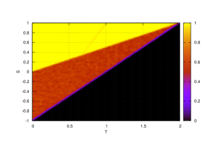
(a) When game started with $10\%$ cooperators at random positions.

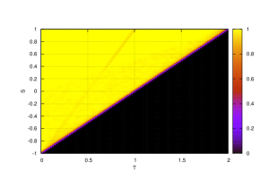
(b) When game started with $25\%$ cooperators at random positions.

Figure 9: Fraction of cooperators on the cycle of length 100 after 10000 generations plotted as a contour for varying $S$ and R.

With this explanation, it is not surprising that, when the game is started with $25\%$ cooperators, the convergence towards the all-cooperate state is more frequent (more than $98\%$) when $2S\leq T\leq S+1$. This is shown in Figure 9(b). This is even more apparent in Figure 10 which shows the contour plotted for the game started with $50\%$ cooperators. In this case, there are clearly only two different behaviours, except for some minor border effects. It can be observed that the average cooperators after 1000 generations is little less than $100\%$ in some places. But, it is clear that the game converges to cooperation before 10000 generations even in these cases.

Finally, all the plots show some minor effects along the line $T=\tfrac{S+1}{2}$ and some noticeable effect along the line $T=S+1$. This is due to the differences in switching probabilities along these borders. Again, this concurs with our analytical results in Section 3.1.4, that cooperators and defectors can coexist in these cases.

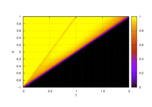
(a) After 1000 generations.

(b) After 10000 generations.

Figure 10: Fraction of cooperators on the cycle of length 100 plotted as a contour for varying $S$ and R, when the game is started with $50\%$ cooperators at random positions.

5.2 Complete graph

For the complete graph, as shown in Section 4, the exact number of cooperators present at the beginning of the game determines whether the game converges to defection or cooperation in the quadrant SH. For this reason, each simulation was started with a fixed number of players. The result obtained are plotted as a contour for varying $S$ and $T$ in Figure 11.

Here again, the results agree with our rigorous analysis. In SG region, the game did not reach a steady state even after 10000 steps. Investigation of the data reveals that the percentage of the cooperator after 10000 steps is close to the value of $\theta^{*}$ obtained in the analysis (e.g. $\theta^{*}=0.49$ when $n=100,T=1.5,$ and $S=0.5$). Also, it is clear that the initial cooperator percentage determines the line in SH region which divides the region with the all-cooperate steady state from the region with the all-defect steady state (e.g. the line is $T\approx S+1$ when $n=100$ and $\theta_{0}=0.5$).

Finally, we note that Santos et al. [15] also produced simulations for complete graphs. Our simulations agree with theirs.

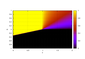
(a) Initial cooperators = $25\%$.

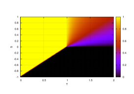
(b) Initial cooperators = $50\%$.

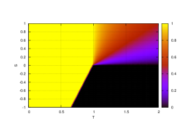
(c) Initial cooperators = $75\%$.

Figure 11: Fractions of cooperators after 10000 generations on the complete graph of size 100 with different initial configurations plotted as a contour for varying $S$ and R.

6 Discussion

We have studied the imitation update rule in two extreme cases of graph topology. First, for the cycle, we have proved that all games converge to either cooperation or defection fast. More precisely, if $T>S+1$, the games converge to the all-defect state fast; and if $T<S+1$, the games converge to the all-cooperate state fast. Even within these regions, the convergence rate for the games is different for different values of the payoffs. It is notable from the analytical results that the closer the point $(S,T)$ is to the line $T=S+1$, the slower the convergence. The fact that the cooperators cannot form a barrier (or a cluster as Nowak and May [9] call it) in PD region seems to suggest that one dimensional graphs cannot help the evolution of cooperation through network reciprocity.

We highlight the fact that, for the complete graph also, all four games converge to cooperation or defection. But the rate of convergence is exponentially slow in $n$ for the SG game. We note that experimental studies, including [9, 15], have wrongly concluded that cooperators and defectors can coexist indefinitely. Our results show that this is true for the complete graph only for some very particular values of $S$ and $T$. In the SG region, as we have proved, the number of cooperators oscillates around a value, $\delta^{*}$, for an exponential amount of time. We showed that convergence to cooperation is more likely after an exponential time if $\delta^{*}$ is closer to $n$, and the convergence to defection is more likely if $\delta^{*}$ is closer to $0$. For some special values of $S$ and $T$, where $\delta^{*}$ is an integer, $\delta^{*}$ cooperators is a steady state. In this state, cooperators and defectors earn equal payoff. We have proved that, for these special values of $S$ and $T$, the convergence to this steady state happens fast.

7 Conclusions and open problems

We have shown that indefinite coexistence of cooperators and defectors is impossible on the cycle, except for some special values of $S$ and $T$. More precisely, the coexistence is only possible for games where $T=S+1$ or $T=(S+1)/2$. Furthermore, we have shown that, for all the games studied, a steady state is reached for cycles in polynomial time. That is, cooperation emerges rapidly when $S+1>T$ and $T\neq(S+1)/2$; defection emerges rapidly when $S+1<T$; and, a steady state with cooperators and defectors is reached rapidly when $T=S+1$ and $T=(S+1)/2$. We also analysed the imitation strategy on complete graphs. The analysis reveals that defection emerges fast for Prisoner’s Dilemma game, and cooperation emerges fast for Harmony game. In the Stag Hunt game, either cooperation or defection emerges fast depending on the initial proportion of cooperators. In the Snowdrift game, a metastable state is reached fast. In this state, the proportion of cooperators fluctuates around a fixed value for exponential time, before converging to cooperation or defection.

It remains as an open question whether there are graphs other than the cycle on which cooperators and defectors cannot coexist. An interesting extension of this work would be to study rigorously the imitation strategy on other graphs, such as trees and grids. In particular, based on simulations presented in [14], regular lattices seem to show very similar, if not the same, behaviour to the complete graphs for the whole $ST$ region. But it does not appear that a similar analysis can be used to prove this.

References

- [1] M. Dyer, L. A. Goldberg, C. Greenhill, G. Istrate, and M. Jerrum, Convergence of the iterated prisoner’s dilemma game, Comb. Probab. Comput. 11 (2002), 135–147.
- [2] W. Feller, An introduction to probability theory and its applications, Wiley, 1968.
- [3] J. Hofbauer and K. Sigmund, Evolutionary games and population dynamics, Cambridge University Press, 1998.
- [4] D. M. Kilgour and N. M. Fraser, A taxonomy of all ordinal games, Theory and Decision 24 (1988), 99–117.
- [5] J. E. Kittock, Emergent conventions and the structure of multi-agent systems, Proceedings of the 1993 Santa Fe Institute Complex Systems Summer School, 1993.
- [6] A. N. Licht, Games commissions play: games of international securities regulation, Yale Journal of International Law 24 (1999), 61–125.
- [7] M. W. Macy and A. Flache, Learning dynamics in social dilemmas, Proceedings of the National Academy of Sciences of the United States of America 99 (2002), 7229–7236.
- [8] E. Mossel and S. Roch, Slow emergence of cooperation for win-stay lose-shift on trees, Mach. Learn. 67 (2007), 7–22.
- [9] M. A. Nowak, Five rules for the evolution of cooperation, Science 314 (2006), 1560–1563.
- [10] M. A. Nowak and R. M. May, Evolutionary games and spatial chaos, Nature 359 (1992), 826–829.
- [11] H. Ohtsuki and M. A. Nowak, Evolutionary games on cycles, Proceedings of the Royal Society B: Biological Sciences 273 (2006), 2249–2256.
- [12] J. M. Pacheco and F. C. Santos, Network dependence of the dilemmas of cooperation, AIP Conference Proceedings 776 (2005), 90–100.
- [13] C. P. Roca, J. A. Cuesta, and A. Sánchez, Imperfect imitation can enhance cooperation, Europhysics Letters 87 (2009), 48005–+.
- [14] , Promotion of cooperation on networks? the myopic best response case, The European Physical Journal B: Condensed Matter and Complex Systems 71 (2009), 587–595.
- [15] F. C. Santos, J. M. Pacheco, and T. Lenaerts, Evolutionary dynamics of social dilemmas in structured heterogeneous populations, PNAS 103 (2006), 3490 – 3494.
- [16] F. C. Santos, J. F. Rodrigues, and J. M. Pacheco, Graph topology plays a determinant role in the evolution of cooperation, Proceedings of the Royal Society B: Biological Sciences 273 (2006), 51–55.
- [17] K. H. Schlag, Why imitate, and if so, how?: A boundedly rational approach to multi-armed bandits, Journal of Economic Theory 78 (1998), 130 – 156.
- [18] D. Snidal, Relative gains and the pattern of international cooperation, The American Political Science Review 85 (1991), 701–726.