The Inglis-Belyaev formula and the hypothesis of the two-quasiparticle excitations

Abstract

The goal of the present work is to revisit the cranking formula of the vibrational parameters, especially its well known drawbacks. The latter can be summarized as spurious resonances or singularities in the behavior of the mass parameters in the limit of unpaired systems. It is found that these problems are simply induced by the presence of two derivatives in the formula. In effect, this formula is based on the hypothesis of contributions of excited states due only to two quasiparticles. But it turns out that this is not the case for the derivatives. We deduce therefore that the derivatives are not well founded in the formula. We propose then simply to suppress these terms from the formula. Although this solution seems to be simplistic, it solves definitively all its inherent problems.

LABEL:LastPage#1

I Introduction

Collective low lying levels of the nucleus are often deduced numerically from the Interacting Bosons Model (IBM) 01 or the Generalized Bohr Hamiltonian (GBH) 1 -1a . Restricting ourselves to the latter we can say that it is built on the basis of seven functions: The collective potential energy of deformation of the nucleus, and for its kinetic-energy part, three mass parameters (also called vibrational parameters ) and three moments of inertia. All these functions depend on the deformation of the nuclear surface. Usually, the deformation energy can be evaluated in the framework of the constrained Hartree-Fock theory (CHF) or by the phenomenological shell correction method. The mass parameters and the moments of inertia are often approximated by the cranking formula 2 -2a or in the self consistent approaches by other models 3 -5 . Most of the self-consistent formulations are based on the adiabatic time dependent Hartree-Fock-Bogolyoubov approximation (ATDHFB) which leads to constrained Hartree-Fock-Bogolioubov (CHFB) calculations 5a -5b in which the so-called Thouless-Valatin corrections are neglected. It is to be noted that there are several self-consistent formulations for the mass parameters in which always some approximations are made (not always the same). Other types of approaches of the mass parameters use the so-called Generator Coordinate Method combined with the Gaussian-Overlap-Approximation (GCM+GOA) 5b1 . Recently new methods have again been developped 5bb -5b2 . This leads to a certain confusion and the problem of the evaluation of the mass parameters remains (up to now) a controversial question as already noticed in Ref.5b2 .

In this paper we will focus exclusively on the mass parameters, especially on the problems induced by the cranking formula, i.e. the ”classical” Inglis-Belyaev formula of the vibrational parameters. Indeed, it is well-known that this formula leads sometimes to inextricable problems when the pairing correlations are taken into account (by means of the BCS model). The transition between normal $\left(\Delta=0\right)$ and superfluid phase $\left(\Delta>\Delta_{0}\approx 0.3MeV\right)$ affects generally the magic nuclei near the spherical shape under the changing of the deformation 11 . The problem occurs sometimes (not always) exactly in these cases for an unpaired system $\Delta\sim 0.$ In that cases the mass parameters take anomalous very large values near a ”critical” deformation close to the spherical shape.

This singular behaviour is well-known and constitutes undoubtedly unphysical effect. It has been early found that these problems are due simply to the presence of the derivatives of $\Delta$ (pairing gap) and $\lambda$ (Fermi level) in the formula. They have been reported many times 1 , 10 -14 in the litterature, but no solution has been proposed. The authors of Ref. 1 and 11 claim that for sufficiently large pairing gaps $\Delta$ the total mass parameter is essentially given by the diagonal part without the derivatives, whereas those of Ref. 14 affirm that the role of the derivatives is by no mean small in the fission process and this leads to contradictory conclusions. Other studies 13 neglect the derivatives without any justification. Some self-consistent calculations met also the same difficulties. For example in Ref. 5c , resonances in mass parameters have also already been noticed. As in the present work they were attributed to the derivative of the gap parameter $\Delta$ near the pairing phase transition. In short, up to now the problem remains unclear.
Curiously, one must point out that contrary to the vibrational parameters, the same formulation (Inglis-Belyaev) for the moments of inertia does not exhibit any explicit dependence on $\Delta$ and $\lambda$ (as the I-B formula does for the mass parameters) and this explains why the I-B formula for the moments of inertia does not meet such problems. This difference appears not so natural and is a part of the motivation of this work. All these problems as well as intensive numerical calculations led us to ask ourselves if the presence of these derivatives is well founded. If this is not the case, their removal should be justified. In fact, the Inglis-Belyaev formula is based on the fundamental hypothesis on contributions of two-quasiparticle states excitations. Rigorously it turns out that the derivatives of $\Delta$ and $\lambda$ do not belong to this type of excitations and this must explain their reject from the formula.
The object of this paper is not so much to tell if this model is good or not or to specify the field of the validity this model, etc… This study is simply and wholly devoted to a correction of the Inglis-Belyaev formula in the light of its fundamental hypothesis.

II Hypothesis of the two-quasiparticle excitations or the cranking Inglis-Belyaev formula.

II.1 Without pairing correlations

The mass (or vibrational) parameters are given by the Inglis formula 1 , 2 :

$$D_{ij}\left\{\beta_{1},.,\beta_{n}\right\}=2\hbar^{2}\sum_{M\neq 0}\frac{\left\langle O\right|\partial\text{ }/\partial\beta_{i}\left|M\right\rangle\left\langle M\right|\partial\text{ }/\partial\beta_{j}\left|O\right\rangle}{E_{M}-E_{O}}$$ (1)

Where $\left|O\right\rangle,\left|M\right\rangle$ are respectively the ground state and the excited states of the nucleus. The quantities $E_{M},E_{O}$ are the associated eigenenergies. In the independent-particle model, whenever the state of the nucleus is assumed to be a Slater determinant (built on single-particle states of the nucleons), the ground state$\left|O\right\rangle$ will be of course the one where all the particles occupy the lowest states. The excited states $\left|M\right\rangle$ will be approached by the one particle-one hole configurations. In that case, Eq. (1) becomes:

$$D_{ij}\left\{\beta_{1},.,\beta_{n}\right\}=2\hbar^{2}{\textstyle\sum\limits_{l>\lambda,k<\lambda}}\frac{\left\langle k\right|\dfrac{\partial}{\partial\beta_{i}}\left|l\right\rangle\left\langle l\right|\dfrac{\partial}{\partial\beta_{i}}\left|k\right\rangle}{\left(\epsilon_{l}-\epsilon_{k}\right)}$$ (2)

where $\left\{\beta_{1},.,\beta_{n}\right\}$ or in short $\left\{\beta\right\}$ is a set of deformation parameters. The single particle states $\left|l\right\rangle,\left|k\right\rangle$ and single particle energies $\epsilon_{l},\epsilon_{k}$ are given by the Schrodinger equation of the independent-particle model 8 , i.e. $H_{sp}\left|\nu\right\rangle=\epsilon_{\nu}\left|\nu\right\rangle$, where $H_{sp}$is the single-particle Hamiltonian). At last $\lambda$ is the Fermi level

Using the properties $\left\langle\nu\right|\partial/\partial\beta\left|\mu\right\rangle=\left\langle\nu\right|\left[\partial/\partial\beta,H_{sp}\right]\left|\mu\right\rangle/\left(\epsilon_{\nu}-\epsilon_{\mu}\right)$ and $\left[\partial/\partial\beta,H_{sp}\right]=\partial H_{sp}/\partial\beta$ Eq.(2) becomes

$$D_{ij}\left\{\beta_{1},.,\beta_{n}\right\}=2\hbar^{2}{\textstyle\sum\limits_{l>\lambda,k<\lambda}}\dfrac{\left\langle k\right|\dfrac{\partial H_{sp}}{\partial\beta_{i}}\left|l\right\rangle\left\langle l\right|\dfrac{\partial H_{sp}}{\partial\beta_{i}}\left|k\right\rangle}{\left(\epsilon_{l}-\epsilon_{k}\right)^{3}}$$ (3)

$H_{sp}$ is the single-particle Hamiltonian and $\lambda$ is the Fermi level.

II.2 With pairing correlations, hypothesis of the two-quasiparticle excitations states

It must be noted that in Eq. (3) the denominator $\epsilon_{l}-\epsilon_{k}$ vanishes in the case where the Fermi level coincides with two or more degenerate levels. This is the major drawback of the formula. It is possible to overcome this difficulty by taking into account the pairing correlations. This can be achieved through the BCS approximation by the following replacements in Eq. (1):
  i) the ground state $\left|O\right\rangle$ by the BCS state $\left|BCS\right\rangle.$
  ii) the excited states $\left|M\right\rangle$ by the two-quasiparticle excitations states $\left|\nu,\mu\right\rangle=\alpha_{\nu}^{+}\alpha_{\mu}^{+}\left|BCS\right\rangle$ (here we consider only the even-even nuclei).
  iii) the energy $E_{O\text{ }}$ by $E_{BCS}$ and $E_{M}$ by the energy of the two quasiparticles, i.e., by $E_{\nu}+E_{\mu}+E_{BCS}$. The BCS state is defined from the ”true” vacuum $\left|0\right\rangle$ by: $\left|BCS\right\rangle=\Pi_{k}\left(u_{k}+\upsilon_{k}a_{k}^{+}a_{\overline{k}}^{+}\right)\left|0\right\rangle$.

$$D_{ij}\left\{\beta_{1},.,\beta_{n}\right\}=2\hbar^{2}\sum_{\nu,\mu}\frac{\left\langle BCS\right|\partial\text{ }/\partial\beta_{i}\left|\nu,\mu\right\rangle\left\langle\nu,\mu\right|\partial\text{ }/\partial\beta_{j}\left|BCS\right\rangle}{E_{\nu}+E_{\mu}}$$ (4)

Where $\left(u_{\nu},\upsilon_{\mu}\right)$ are the usual amplitudes of probability and

$$E_{\nu}=\sqrt{\left(\epsilon_{\nu}-\lambda\right)^{2}+\Delta^{2}}$$ (5)

is the so-called quasiparticle energy.
As shown by Belyaev 6 or as detailed in appendix tha above formula can be written in an other form:

$$D_{ij}\left\{\beta_{1},.,\beta_{n}\right\}=2\hbar^{2}{\displaystyle\sum_{\nu}}{\displaystyle\sum_{\mu\neq\nu}}\left(u_{\nu}\upsilon_{\mu}+u_{\mu}\upsilon_{\nu}\right)^{2}\dfrac{\left\langle\nu\right|\dfrac{\partial}{\partial\beta_{i}}\left|\mu\right\rangle\left\langle\mu\right|\dfrac{\partial}{\partial\beta_{j}}\left|\nu\right\rangle}{E_{\nu}+E_{\mu}}+2\hbar^{2}\underset{\nu}{{\displaystyle\sum}}\frac{1}{2E_{\nu}}\frac{1}{\upsilon_{\nu}^{2}}\frac{\partial u_{\nu}}{\partial\beta_{i}}\frac{\partial u_{\nu}}{\partial\beta_{j}}$$ (6)

Beside this formula, there is an other more convenient formulation due to Bes 7 modified slightly by the authors of Ref. 1 where the derivatives $\partial u_{\nu}/\partial\beta_{i},\partial u_{\nu}/\partial\beta_{j}$ of Eq.(6) are explitly performed (see also the details in the appendix of the present paper):

$$D_{ij}\left\{\beta_{1},.,\beta_{n}\right\}=2\hbar^{2}{\displaystyle\sum_{\nu}}{\displaystyle\sum_{\mu\neq\nu}}\frac{\left(u_{\nu}\upsilon_{\mu}+u_{\mu}\upsilon_{\nu}\right)^{2}}{\left(E_{\nu}+E_{\mu}\right)^{3}}\left\langle\nu\right|\dfrac{\partial H_{sp}}{\partial\beta_{i}}\left|\mu\right\rangle\left\langle\mu\right|\dfrac{\partial H_{sp}}{\partial\beta_{j}}\left|\nu\right\rangle+2\hbar^{2}\underset{\nu}{{\displaystyle\sum}}\dfrac{\Delta^{2}}{8E_{\nu}^{5}}R_{i}^{\nu}R_{j}^{\nu}$$ (7)

here the most important quantity concerned by the subject of this paper is $R_{i}^{\nu}$ (once again see formula (28) in appendix how this quantity is obtained):

$$R_{i}^{\nu}=-\left\langle\nu\right|\frac{\partial H_{sp}}{\partial\beta_{i}}\left|\nu\right\rangle+\dfrac{\partial\lambda}{\partial\beta_{i}}+\frac{\left(\epsilon_{\nu}-\lambda\right)}{\Delta}\dfrac{\partial\Delta}{\partial\beta_{i}}$$ (8)

The two quantities of the r.h.s of Eq. (6) and (7) are in the adopted order, the so-called ”non-diagonal” and the ”diagonal” parts of the mass parameters. The derivatives are contained in the above diagonal term $R_{i}^{\nu}$. In other papers, the cranking formula is usually cast under a slightly different form.

All these formulae (4), (6), (7) and others are equivalent.
The derivatives contained in Eq (8) can be then actually calculated as in the Ref. 11 , 1 with the help of the following formulae.

$$\frac{\partial\lambda}{\partial\beta_{i}}=\frac{ac_{\beta_{i}}+bd_{\beta_{i}}}{a^{2}+b^{2}}$$ (9)

$$\frac{\partial\Delta}{\partial\beta_{i}}=\frac{bc_{\beta_{i}}-ad_{\beta_{i}}}{a^{2}+b^{2}}$$ (10)

with

$$a=\underset{\nu}{{\displaystyle\sum}}\Delta E_{\nu}^{-3},\text{ \ }b=\underset{\nu}{{\displaystyle\sum}}(\epsilon_{\nu}-\lambda)E_{\nu}^{-3},$$ (11)

$$c_{\beta_{i}}=\underset{\nu}{{\displaystyle\sum}}\Delta\left\langle\nu\right|\dfrac{\partial H_{sp}}{\partial\beta_{i}}\left|\nu\right\rangle E_{\nu}^{-3},\text{ \ }d_{\beta_{i}}=\underset{\nu}{{\displaystyle\sum}}(\epsilon_{\nu}-\lambda)\left\langle\nu\right|\dfrac{\partial H_{sp}}{\partial\beta_{i}}\left|\nu\right\rangle E_{\nu}^{-3}$$ (12)

These equations can be easily derived through the well known properties of the implicit functions. In the following the expression ”the derivatives” means simply the both derivatives given by Eq. (9) and (10).

In the simple BCS theory the gap parameters $\Delta$ and the Fermi level $\lambda$ are solved from the following BCS equations (13) and (14) as soon as the single-particle spectrum $\left\{\epsilon_{\nu}\right\}$ is known.

$$\dfrac{2}{G}=\underset{\nu=1}{\overset{N_{P}}{\sum}}\frac{1}{\sqrt{\left(\epsilon_{\nu}-\lambda\right)^{2}+\Delta^{2}}}$$ (13)

$$N\text{ or }Z=\underset{\nu=1}{\overset{N_{P}}{\sum}}\left(1-\frac{\epsilon_{\nu}-\lambda}{\sqrt{\left(\epsilon_{\nu}-\lambda\right)^{2}+\Delta^{2}}}\right)$$ (14)

($N_{P}$ is the number of pairs of particles in numerical calculations). Of course, from equations (13) and (14) the deformation dependence of the eigenenergies $\epsilon_{\nu}(\beta)$ involves the ones of $\Delta$ and $\lambda$.
Formally, the solution of Eq.(13) and (14) amounts to express $\Delta$ and $\lambda$ as functions of the set of the energy levels $\left\{\epsilon_{\nu}\right\}$.

II.3
Paradox of the formula in an umpaired system

It is well known that the BCS equations have non-trivial solutions only above a critical value of the strength $G$ of the pairing interaction. The trivial solution corresponds theoretically to the value $\Delta=0$ of an unpaired system. In this case, the mass parameters given by (6) or (7) must reduce to the ones of the formula (3), i.e. the cranking formula of the independent-particle model. Indeed, when $\Delta=0$ it is quite clear that:

$E_{\nu}=\sqrt{\left(\epsilon_{\nu}-\lambda\right)^{2}+\Delta^{2}}\rightarrow E_{\nu}=\left|\epsilon_{\nu}-\lambda\right|$

$u_{\nu},\upsilon_{\nu}\rightarrow$ $0$ $or$ $1$ therefore in Eq.(7) $\left(u_{\nu}\upsilon_{\mu}+u_{\mu}\upsilon_{\nu}\right)^{2}\rightarrow$ $0$ $or$ $1$

In accordance with the above assumption $\left(u_{\nu}\upsilon_{\mu}+u_{\mu}\upsilon_{\nu}\right)^{2}=$ $0$ $or$ $1$, we can define $\nu$ and $\mu$ in a such way $\epsilon_{\nu}>\lambda$ and $\epsilon_{\mu}<\lambda$ therefore $E_{\nu}+E_{\mu}=\left|\epsilon_{\nu}-\lambda\right|+\left|\epsilon_{\mu}-\lambda\right|$ $=\epsilon_{\nu}-\lambda+\lambda-\epsilon_{\mu}=\epsilon_{\nu}-\epsilon_{\mu}$
so that it is easy to see that the non-diagonal part of the right hand side of  Eq.(7) reduces effectively to Eq. (3), i.e.:

$2\hbar^{2}{\displaystyle\sum_{\nu}}{\displaystyle\sum_{\mu\neq\nu}}\frac{\left(u_{\nu}\upsilon_{\mu}+u_{\mu}\upsilon_{\nu}\right)^{2}}{\left(E_{\nu}+E_{\mu}\right)^{3}}\left\langle\nu\right|\tfrac{\partial H_{sp}}{\partial\beta_{i}}\left|\mu\right\rangle\left\langle\mu\right|\tfrac{\partial H_{sp}}{\partial\beta_{j}}\left|\nu\right\rangle\rightarrow 2\hbar^{2}{\textstyle\sum\limits_{\nu>\lambda,\mu<\lambda}}\tfrac{\left\langle\nu\right|\tfrac{\partial H_{sp}}{\partial\beta_{i}}\left|\mu\right\rangle\left\langle\mu\right|\tfrac{\partial H_{sp}}{\partial\beta_{i}}\left|\nu\right\rangle}{\left(\epsilon_{\nu}-\epsilon_{\mu}\right)^{3}}$
This implies the important fact that in this limit ($\Delta\rightarrow 0$), the diagonal part (i.e. the second term) of the r.h.s. of Eq. (7) must vanish, i.e. in other words:

$2\hbar^{2}\underset{\nu}{{\displaystyle\sum}}\tfrac{\Delta^{2}}{8E_{\nu}^{5}}R_{i}^{\nu}R_{j}^{\nu}$ $\rightarrow 0$ when $\Delta\rightarrow 0$
However in practice in some rare cases of the pairing phase transtion this does not occur because it happens that this term diverges near the breakdown of the pairing correlations, i.e., in practice for very small values of $\Delta(\sim 0)$ (see numerical example in the text below). This constitutes really a contradiction and a paradox in this formula.
In the quantity $R_{i}^{\nu}$ of Eq (8) the diagonal matrix elements $\left\langle\nu\right|\partial H_{sp}/\partial\beta_{i}\left|\nu\right\rangle$ are finite and relatively small, it is then clear that it is the derivatives $\partial\Delta/\partial\beta_{i}$ and $\partial\lambda/\partial\beta_{i}$ which cause the problem. These features have been checked in numerical calculations. In this respect, the formulae (9) and (10) which give these derivatives are subject to a major drawback because their common denominator, i.e. $a^{2}+b^{2}$ can accidentally cancel. Let us study briefly this situation. In effect, this can be easily explained because in unpaired situation we must have $\Delta\sim 0,$ involving $a\sim 0$ in Eq. (11). In addition, $b$ is defined as a sum of postive and negative values depending on whether the terms are below or above the Fermi level. Therefore, it could happen accidentally that $b\sim 0$ in Eq (11) involving serious drawbacks or at least numerical instabilities.

III Quantities such as $\Delta$ and $\lambda$ are not consistent with the hypothesis of the Inglis-Belyaev formula.

III.1 Basic hypothesis of the Inglis-Belyaev formula and simplification of the formula

In the independent-particle approximation the contributions to the mass parameters are simply due to one particle-one hole excitations. Thus in the formulae (2) or (3) the particle-hole excitations are denoted by the single-particle states $k$ and $l$. When the pairing correlations are taken into account, the contributions are supposed due only to two-quasiparticle excitations states $\left(\nu,\overline{\mu}\right)$ $\left\{\mu\neq\nu\right\}$ in Eq. which gives rise to the first term of Eq.(7). The second term of this formula is due to the derivatives of the probability amplitudes and has to be interpreted as two quasiparticle excitations of the type $\left(\nu,\overline{\nu}\right)$. However this is not true for all the terms entering into the product of the quantities $R_{i}^{\nu},R_{j}^{\nu}$ . Let us re-focus onto the formula (7) in which we will replace in the second sum the quantity $\Delta$ by its equivalent from the identity $\Delta=2u_{\nu}\upsilon_{\nu}E_{\nu}$. After simplification of the coefficient of $R_{i}^{\nu}R_{j}^{\nu}$ we obtain:

$$D_{ij}\left\{\beta_{1},.,\beta_{n}\right\}=2\hbar^{2}{\displaystyle\sum_{\nu}}{\displaystyle\sum_{\mu\neq\nu}}\frac{\left(u_{\nu}\upsilon_{\mu}+u_{\mu}\upsilon_{\nu}\right)^{2}}{\left(E_{\nu}+E_{\mu}\right)^{3}}\left\langle\nu\right|\dfrac{\partial H_{sp}}{\partial\beta_{i}}\left|\mu\right\rangle\left\langle\mu\right|\dfrac{\partial H_{sp}}{\partial\beta_{j}}\left|\nu\right\rangle+2\hbar^{2}\underset{\nu}{{\displaystyle\sum}}\dfrac{\left(2u_{\nu}\upsilon_{\nu}\right)^{2}}{8E_{\nu}^{3}}R_{i}^{\nu}R_{j}^{\nu}$$ (15)

The fundamental point is in this way it is clear that all the quantities in Eq. (15) are associated to quasiparticle states $\nu$ and $\mu$ except the derivative of $\Delta$ and $\lambda.$  Quantities such as $\Delta$ and $\lambda$ appearing in $\left(R_{i}^{\nu},R_{j}^{\nu}\right)$ (see Eq. (8)) which are deduced from Eq. (13)-(14) are due to all the spectrum, they are clearly not specifically linked to these two particular states (otherwise indices $\nu$ and $\mu$ should appear with these quantities). Therefore they cannot be really considered as contributions due to two quasiparticle excitation states which is the basic hypothesis of the Inglis-Belyaev formula. Therefore they cannot be taken into account.
With this additional assumption, the element $R_{i}^{\nu}$ must reduce to nothing but a simple matrix element:

$$R_{i}^{\nu}=-\left\langle\nu\right|\frac{\partial H_{sp}}{\partial\beta_{i}}\left|\nu\right\rangle$$ (16)

Consequently this contributes to simplify greatly the formula (15) which becomes:

$$D_{ij}\left\{\beta_{1},.,\beta_{n}\right\}=2\hbar^{2}{\displaystyle\sum_{\nu}}{\displaystyle\sum_{\mu\neq\nu}}\left(u_{\nu}\upsilon_{\mu}+u_{\mu}\upsilon_{\nu}\right)^{2}\frac{\left\langle\nu\right|\dfrac{\partial H_{sp}}{\partial\beta_{i}}\left|\mu\right\rangle\left\langle\mu\right|\dfrac{\partial H_{sp}}{\partial\beta_{j}}\left|\nu\right\rangle}{\left(E_{\nu}+E_{\mu}\right)^{3}}+2\hbar^{2}\underset{\nu}{{\displaystyle\sum}}\left(2u_{\nu}\upsilon_{\nu}\right)^{2}\frac{\left\langle\nu\right|\dfrac{\partial H_{sp}}{\partial\beta_{i}}\left|\nu\right\rangle^{2}}{\left(2E_{\nu}\right)^{3}}$$ (17)

It is to be noted that the missing term $(\mu=\nu)$ in the double sum is precisely the contribution of the simple sum of the r.h.s of Eq. (17). Therefore, the formula (17) can be reformulated in a compact form:

$$D_{ij}\left\{\beta_{1},.,\beta_{n}\right\}=2\hbar^{2}{\displaystyle\sum_{\nu}}{\displaystyle\sum_{\mu}}\left(u_{\nu}\upsilon_{\mu}+u_{\mu}\upsilon_{\nu}\right)^{2}\frac{\left\langle\nu\right|\dfrac{\partial H_{sp}}{\partial\beta_{i}}\left|\mu\right\rangle\left\langle\mu\right|\dfrac{\partial H_{sp}}{\partial\beta_{j}}\left|\nu\right\rangle}{\left(E_{\nu}+E_{\mu}\right)^{3}}$$ (18)

In this more ”symmetric” form, this formula looks like more naturally to the Inglis-Belyaev formula of the moments of inertia which does not contain dependence on the derivatives of $\Delta$ and $\lambda$.

The ”new” formula corrects the previous paradox because in the case of the phase transition $\Delta\rightarrow 0$, we will have in this limit for the diagonal terms $\nu=\mu,$ $u_{\nu}\upsilon_{\nu}+u_{\nu}\upsilon_{\nu}=0$ for any $\nu$ and due to the fact that the corresponding matrix element $\left\langle\nu\right|\partial H_{sp}/\partial\beta_{i}\left|\nu\right\rangle$ is finite the second term of Eq. (17) tends uniformly toward zero so that Eq. (17) reduces in this case to the equation of the unpaired system (3) without any problem.

IV Illustration of the application of the Inglis Belyaev formula in the case where the singularity occurs

This is illustrated in Fig. 1 by the behaviour of the vibrational parameter $B_{\beta\beta}(\beta,\gamma=0)$ as a function of the Bohr parameter in the case of the magic nuclei ${}_{54}^{136}$Xe₈₂. These calculations have been performed for the both formulae (7) and (17), i.e., respectively with and without the derivatives $\partial\lambda/\partial\beta$ and $\partial\Delta/\partial\beta$. The resonance (singularity) $B_{\beta\beta}\sim 7000000\hbar^{2}MeV^{-1}$ occurs near the deformation $\beta=0.09$ for the formula with the derivatives. This happens even if $\Delta$ is very close to $0.$ Between $\beta=0$ and $\beta=0.15$ the formula without derivatives gives small (finite) values ($B_{\beta\beta}\sim 25\hbar^{2}MeV^{-1}$). These very small values of the independent particle model are due to the collapse of the pairing correlations. In addition, during the phase transition, i.e., for $0.1\lesssim\Delta\lesssim 0.2,$ the vibrational parameters increase up to the important value $B_{\beta\beta}\sim 500\hbar^{2}MeV^{-1}$. We have checked that this is due to a pseudo crossing levels near the Fermi level. However, in this respect we have futhermore checked carefully that there is absolutely no crossing levels near the singularity. Thus the singularity is not a consequence of a crossing levels as it is often claimed 10 . As said before the explanation comes from the fact that in Eq. (9) and (10) the denominator simply cancels. This demonstrates the weakness of the old formula (7) with respect to that proposed in this paper, that is Eq. (17).

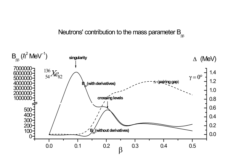
Figure 1: Neutron contribution to the mass parameters $B_{\beta\beta}$ for the magic nucleus ${}_{54}^{136}Xe_{82}$; The calculations are performed within the cranking formula including the derivatives and for the same formula without derivating; Note the quasi divergence (singularity) of the version with derivatives near the deformation $\beta=0.1$

V Conclusion

In some rare but important illustrative cases the application of the Inglis-Belyaev formula to the mass parameters reveals incontestable weaknesses in the limit of unpaired systems $\Delta\rightarrow 0$. In effect, this formula leads straightforwardly to a major contradiction, that is, not only it does not reduce to the one of the unpaired system in the case $\Delta=0$ (which is already a contradictory fact) but even gives unphysical (singular) values. It has been reported in the litterature that self-consistent calculations meet also the same kind of problems (see text). After extensive calculations within the Inglis-Belyaev formula, we realized that these problems are inherent to a spurious presence of the derivatives of $\Delta$ and $\lambda$ in the formula. This led us to ”revise” the conception of this formula simply by removing the derivatives which are not consistent with the basic hypothesis of the formula, that is to say with two quasiparticle excitation states. This is the reason why our proposal cannot be considered as a simple recipe to the limit $\Delta=0$ but as a well founded rectification of the formula which is thus no more subject to the cited problems and reduces naturally to that of the unpaired system in the limit $\Delta\rightarrow 0$.

Appendix A The cranking formula with pairing correlations

We have to calculate the matrix element of the type $\left\langle n,m\right|\partial$ $/\partial\beta_{i}\left|BCS\right\rangle$ which appears in Eq. (4) of the text, i.e.:

$D_{ij}\left\{\beta_{1},.,\beta_{n}\right\}=2\hbar^{2}\sum_{\nu,\mu}\frac{\left\langle BCS\right|\partial\text{ }/\partial\beta_{i}\left|\nu,\mu\right\rangle\left\langle\nu,\mu\right|\partial\text{ }/\partial\beta_{j}\left|BCS\right\rangle}{E_{\nu}+E_{\mu}}$
keeping in mind however that the differential operator acts not only on the wave functions of the BCS state but also on the occupations probabilities $u_{k},\upsilon_{k}$ (of the BCS state) which also depend on the deformation parameter $\beta_{i}$ we have to write.

$\dfrac{\partial}{\partial\beta_{i}}=\left(\dfrac{\partial}{\partial\beta_{i}}\right)_{wave\text{ }func}+\left(\dfrac{\partial}{\partial\beta_{i}}\right)_{occup.prob}$
We must therefore to evaluate successively two types of matrix elements

A.1 Calculation of the first type of matrix elements

For one particle operator we have in second quantization representation:
$\left(\dfrac{\partial}{\partial\beta_{i}}\right)_{wave\text{ }func}=\sum_{\nu,\mu}\left\langle\nu\right|\dfrac{\partial}{\partial\beta_{i}}\left|\mu\right\rangle a_{\nu}^{+}a_{\mu}$
Applying this operator on the paired system and using the inverse of the Bogoliubov-Valatin transformation:
$a_{\nu}=(u_{\nu}\alpha_{\nu}+\upsilon_{\nu}\alpha_{\overline{\nu}}^{+}),a_{\nu}^{+}=(u_{\nu}\alpha_{\nu}^{+}+\upsilon_{\nu}\alpha_{\overline{\nu}})$
We find:

$$\left(\dfrac{\partial}{\partial\beta_{i}}\right)_{wave\text{ }func}\left|BCS\right\rangle=\sum_{\nu,\mu}\left\langle\nu\right|\dfrac{\partial}{\partial\beta_{i}}\left|\mu\right\rangle a_{\nu}^{+}a_{\mu}\left|BCS\right\rangle$$ (19)

$=\sum_{\nu,\mu}\left\langle\nu\right|\dfrac{\partial}{\partial\beta_{i}}\left|\mu\right\rangle(u_{\nu}\alpha_{\nu}^{+}+\upsilon_{\nu}\alpha_{\overline{\nu}})(u_{\mu}\alpha_{\mu}+\upsilon_{\mu}\alpha_{\overline{\mu}}^{+})\left|BCS\right\rangle=\sum_{\nu,\mu}\left\langle\nu\right|\dfrac{\partial}{\partial\beta_{i}}\left|\mu\right\rangle(u_{\nu}\alpha_{\nu}^{+}+\upsilon_{\nu}\alpha_{\overline{\nu}})\upsilon_{\mu}\alpha_{\overline{\mu}}^{+}\left|BCS\right\rangle$ because $\alpha_{\mu}\left|BCS\right\rangle=0$
Therefore

$$\left(\dfrac{\partial}{\partial\beta_{i}}\right)_{wave\text{ }func}\left|BCS\right\rangle=\sum_{\nu,\mu}\left\langle\nu\right|\dfrac{\partial}{\partial\beta_{i}}\left|\mu\right\rangle\left\{u_{\nu}\alpha_{\nu}^{+}\upsilon_{\mu}\alpha_{\overline{\mu}}^{+}\left|BCS\right\rangle+\upsilon_{\nu}\alpha_{\overline{\nu}}\upsilon_{\mu}\alpha_{\overline{\mu}}^{+}\left|BCS\right\rangle\right\}$$ (20)

We must notice that for the term $\nu=\mu$ we will have the contribution $\left\langle\nu\right|\dfrac{\partial}{\partial\beta_{i}}\left|\nu\right\rangle\left\{u_{\nu}\upsilon_{\nu}\alpha_{\nu}^{+}\alpha_{\overline{\nu}}^{+}\left|BCS\right\rangle+\upsilon_{\nu}^{2}\left|BCS\right\rangle\right\}$ which is a mixing of a two quasparticle-state with a BCS state. Because the state given by Eq. (19) must represent only two quasiparticle excitation, we have to exclude the contribution due to the term $\nu=\mu$ from the sum of this equation. This restriction leads to the following formula:

$$\left(\dfrac{\partial}{\partial\beta_{i}}\right)_{wave\text{ }func}\left|BCS\right\rangle=\sum_{\nu\neq\mu}\left\langle\nu\right|\dfrac{\partial}{\partial\beta_{i}}\left|\mu\right\rangle(u_{\nu}\upsilon_{\mu}\alpha_{\nu}^{+}\alpha_{\overline{\mu}}^{+})\left|BCS\right\rangle$$ (21)

It will be noted that the term $\upsilon_{\nu}\alpha_{\overline{\nu}}\upsilon_{\mu}\alpha_{\overline{\mu}}^{+}\left|BCS\right\rangle$ vanishes for $\nu\neq\mu$ in the r.h.s of Eq. (20). We then calculate then the first type of matrix elements:

$$I_{1}=\left\langle n,m\right|\sum_{\nu\neq\mu}\left\langle\nu\right|\dfrac{\partial}{\partial\beta_{i}}\left|\mu\right\rangle u_{\nu}\upsilon_{\mu}\alpha_{\nu}^{+}\alpha_{\overline{\mu}}^{+}\left|BCS\right\rangle$$ (22)

The above form of the formula suggests that the excited states must be of the form $\left|n,m\right\rangle=\alpha_{k}^{+}\alpha_{\overline{l}}^{+}\left|BCS\right\rangle=\left|k,\overline{l}\right\rangle$.
We obtain then:
$I_{1}=\left\langle BCS\right|\alpha_{\overline{l}}\alpha_{k}\sum_{\nu\neq\mu}\left\langle\nu\right|\dfrac{\partial}{\partial\beta_{i}}\left|\mu\right\rangle u_{\nu}\upsilon_{\mu}\alpha_{\nu}^{+}\alpha_{\overline{\mu}}^{+}\left|BCS\right\rangle$
$=\sum_{\nu\neq\mu}\left\langle\nu\right|\dfrac{\partial}{\partial\beta_{i}}\left|\mu\right\rangle u_{\nu}\upsilon_{\mu}\left\langle BCS\right|\alpha_{\overline{l}}\alpha_{k}\alpha_{\nu}^{+}\alpha_{\overline{\mu}}^{+}\left|BCS\right\rangle$
We use the following usual fermions anticommutation relations:
$\left\{\alpha_{k},\alpha_{l}\right\}=\left\{\alpha_{k}^{+},\alpha_{l}^{+}\right\}=0,$    $\left\{\alpha_{k},\alpha_{l}^{+}\right\}=\delta_{kl}$
Thus the quantity between brakets of the BCS sate gives:
$\left\langle BCS\right|\alpha_{\overline{l}}\alpha_{k}\alpha_{\nu}^{+}\alpha_{\overline{\mu}}^{+}\left|BCS\right\rangle=\left(\delta_{l\mu}\delta_{\nu k}-\delta_{\overline{\mu}k}\delta_{\nu\overline{l}}\right)$
We obtain:
$I_{1}=\sum_{\nu\neq\mu}\left\langle\nu\right|\dfrac{\partial}{\partial\beta_{i}}\left|\mu\right\rangle u_{\nu}\upsilon_{\mu}\left(\delta_{l\mu}\delta_{\nu k}-\delta_{\overline{\mu}k}\delta_{\nu\overline{l}}\right)=\left\langle k\right|\dfrac{\partial}{\partial\beta_{i}}\left|l\right\rangle u_{k}\upsilon_{l}-\left\langle\overline{l}\right|\dfrac{\partial}{\partial\beta_{i}}\left|\overline{k}\right\rangle u_{\overline{l}}\upsilon_{\overline{k}}$   with   $k\neq l$ Because indexes of brakets must be different in Eq(22).
Noting that if $\widehat{T}$ is the time-reversal conjugation operator we must have for any operator $\hat{O}$
$\left\langle p\right|\hat{O}\left|q\right\rangle=\left\langle\widehat{T}p\right|\widehat{T}\hat{O}\widehat{T}^{-1}\left|\widehat{T}q\right\rangle^{\ast}$
Applying this result for our case and assuming that $\partial/\partial\beta_{i}$ is time-even, i.e. $\widehat{T}\left(\partial/\partial\beta_{i}\right)\widehat{T}^{-1}=\partial/\partial\beta_{i}$, we get:
$\left\langle\overline{l}\right|\dfrac{\partial}{\partial\beta_{i}}\left|\overline{k}\right\rangle=\left\langle\widehat{T}\overline{l}\right|\widehat{T}\dfrac{\partial}{\partial\beta_{i}}\widehat{T}^{-1}\left|\widehat{T}\overline{k}\right\rangle^{\ast}=\left\langle k\right|\dfrac{\partial}{\partial\beta_{i}}\left|l\right\rangle$
Moreover, using the usual phase convention
$u_{\overline{l}}=u_{l}$, $\upsilon_{\overline{k}}=-\upsilon_{k}$
we deduce :
$I_{1}=\left\langle k\right|\dfrac{\partial}{\partial\beta_{i}}\left|l\right\rangle u_{k}\upsilon_{l}+\left\langle k\right|\dfrac{\partial}{\partial\beta_{i}}\left|l\right\rangle u_{l}\upsilon_{k}=\left(u_{k}\upsilon_{l}+u_{l}\upsilon_{k}\right)\left\langle k\right|\dfrac{\partial}{\partial\beta_{i}}\left|l\right\rangle$  
Taking into account that the brakets states in Eq (21) must be different, the final result for $I_{1}$ given (22) will take the following form:

$$I_{1}=\left\langle k,\overline{l}\right|\left(\frac{\partial}{\partial\beta_{i}}\right)_{wave\text{ }func}\left|BCS\right\rangle=\left(u_{k}\upsilon_{l}+u_{l}\upsilon_{k}\right)\left\langle k\right|\frac{\partial}{\partial\beta_{i}}\left|l\right\rangle\ \ with\ \ k\neq l$$ (23)

Let be $H_{sp}$ the single-particle Hamiltonian and

$$H^{\prime}={\textstyle\sum_{\nu,\mu}}\left\langle\nu\right|\left(H_{sp}-\lambda\right)\left|\mu\right\rangle a_{\nu}^{+}a_{\mu}-G{\textstyle\sum_{\nu,\mu>0}}a_{\nu}^{+}a_{\overline{\nu}}^{+}a_{\overline{\mu}}a_{\mu}$$

the nuclear paired BCS Hamiltonian with the constraint on the particle number. Writing this Hamiltonian in the well-known quasiparticles representation $H^{\prime}=E_{BCS}+{\textstyle\sum_{\nu}}E_{\nu}\alpha_{\nu}^{+}\alpha_{\nu}+residual$ $qp$ $interaction$, neglecting (as usual) the latter term and using Eq. (21) it is quite easy to establish the following identity

$$\left\langle k,\overline{l}\right|\left[H^{\prime},\left(\dfrac{\partial}{\partial\beta_{i}}\right)_{wave\text{ }func}\right]\left|BCS\right\rangle=-\left\langle k,\overline{l}\right|\left(\dfrac{\partial H^{\prime}}{\partial\beta_{i}}\right)_{wave\text{ }func}\left|BCS\right\rangle=\left(E_{k,\overline{l}}-E_{BCS}\right)\left\langle k,\overline{l}\right|\left(\dfrac{\partial}{\partial\beta_{i}}\right)_{wave\text{ }func}\left|BCS\right\rangle$$

where the eigenenergies $E_{k,\overline{l}}$ corresponding to the excited states $\left|k,\overline{l}\right\rangle$ are given by $E_{k,\overline{l}}=E_{BCS}+E_{k}+E_{l}$
so that:

$$\left\langle k,\overline{l}\right|\left(\dfrac{\partial}{\partial\beta_{i}}\right)_{wave\text{ }func}\left|BCS\right\rangle=-\dfrac{\left\langle k,\overline{l}\right|\left(\dfrac{\partial H^{\prime}}{\partial\beta_{i}}\right)_{wave\text{ }func}\left|BCS\right\rangle}{E_{k,\overline{l}}-E_{BCS}}=-\dfrac{\left\langle k,\overline{l}\right|\left(\dfrac{\partial H^{\prime}}{\partial\beta_{i}}\right)_{wave\text{ }func}\left|BCS\right\rangle}{E_{k}+E_{l}}$$

Due to the fact that the pairing strength $G$ does not depend on the nuclear deformation, it is clear from the expression of $H^{\prime}$(in the particles representation) that $\partial H^{\prime}/\partial\beta_{i}=\partial\left(H_{sp}-\lambda\right)/\partial\beta_{i}$ Therefore $\left\langle k,\overline{l}\right|\left(\partial H^{\prime}/\partial\beta_{i}\right)_{wave\text{ }func}\left|BCS\right\rangle=\left\langle k,\overline{l}\right|\left(\partial H_{sp}/\partial\beta_{i}\right)\left|BCS\right\rangle-\partial\lambda/\partial\beta_{i}\langle k,\overline{l}\left|BCS\right\rangle=\left\langle k,\overline{l}\right|\left(\partial H_{sp}/\partial\beta_{i}\right)\left|BCS\right\rangle$
Here we have $\langle k,\overline{l}\left|BCS\right\rangle=0$ because excited states and bcs state are supposed orthogonal.
Again using the second quantization formalism $\left(\partial H_{sp}/\partial\beta_{i}\right)=\sum_{\nu\neq\mu}\left\langle\nu\right|\left(\partial H_{sp}/\partial\beta_{i}\right)\left|\mu\right\rangle a_{\nu}^{+}a_{\mu}$ and performing then exactly the same transformations as before for $\sum_{\nu\neq\mu}\left\langle\nu\right|\partial/\partial\beta_{i}\left|\mu\right\rangle a_{\nu}^{+}a_{\mu}$ but this time with $\sum_{\nu\neq\mu}\left\langle\nu\right|\partial H_{sp}/\partial\beta_{i}\left|\mu\right\rangle a_{\nu}^{+}a_{\mu}$ we will obtain in the same manner a new form for Eq. (23):

$$I_{1}=I_{1}(k,l)=\left\langle k,\overline{l}\right|\left(\frac{\partial}{\partial\beta_{i}}\right)_{wave\text{ }func}\left|BCS\right\rangle=-\frac{\left(u_{k}\upsilon_{l}+u_{l}\upsilon_{k}\right)}{E_{k}+E_{l}}\left\langle k\right|\frac{\partial H_{sp}}{\partial\beta_{i}}\left|l\right\rangle\ \ with\ \ k\neq l$$ (24)

A.2 Calculation of the second type of matrix elements

Recalling that the BCS state is given by: $\left|BCS\right\rangle=\Pi_{k}\left(u_{k}+\upsilon_{k}a_{k}^{+}a_{\overline{k}}^{+}\right)\left|0\right\rangle$ and differentiating this state with respect to the probabilty amplitudes, we obtain:
$\left(\dfrac{\partial}{\partial\beta_{i}}\right)_{occup.prob}\left|BCS\right\rangle=\sum_{\tau}(\dfrac{\partial u_{\tau}}{\partial\beta_{i}}+\dfrac{\partial\upsilon_{\tau}}{\partial\beta_{i}}a_{\tau}^{+}a_{\overline{\tau}}^{+})\prod_{k\neq\tau}(u_{k}+\upsilon_{k}a_{k}^{+}a_{\overline{k}}^{+})\left|0\right\rangle$
We use the evident property:
$\prod_{k\neq\tau}(u_{k}+\upsilon_{k}a_{k}^{+}a_{\overline{k}}^{+})\left|0\right\rangle$ $=(u_{\tau}+\upsilon_{\tau}a_{\tau}^{+}a_{\overline{\tau}}^{+})^{-1}\left|BCS\right\rangle$
Therefore:
$\left(\dfrac{\partial}{\partial\beta_{i}}\right)_{occup.prob}\left|BCS\right\rangle=\sum_{\tau}\left[(\dfrac{\partial u_{\tau}}{\partial\beta_{i}}+\dfrac{\partial\upsilon_{\tau}}{\partial\beta_{i}}a_{\tau}^{+}a_{\overline{\tau}}^{+})(u_{\tau}+\upsilon_{\tau}a_{\tau}^{+}a_{\overline{\tau}}^{+})^{-1}\right]\left|BCS\right\rangle$
Making an expansion of the inverse operator in $a_{\tau}^{+}a_{\overline{\tau}}^{+}$ :
$\left(\dfrac{\partial}{\partial\beta_{i}}\right)_{occup.prob}\left|BCS\right\rangle=\sum_{\tau}\left[(\dfrac{\partial u_{\tau}}{\partial\beta_{i}}+\dfrac{\partial\upsilon_{\tau}}{\partial\beta_{i}}a_{\tau}^{+}a_{\overline{\tau}}^{+})u_{\tau}^{-1}(1-\upsilon_{\tau}u_{\tau}^{-1}a_{\tau}^{+}a_{\overline{\tau}}^{+}+\left(\upsilon_{\tau}u_{\tau}^{-1}a_{\tau}^{+}a_{\overline{\tau}}^{+}\right)^{2}+...)\right]\left|BCS\right\rangle$
using the inverse of the Bogoliubov-Valatin transformation:
$a_{\tau}^{+}=(u_{\tau}\alpha_{\tau}^{+}+\upsilon_{\tau}\alpha_{\overline{\tau}})$
We find for the quantity $a_{\tau}^{+}a_{\overline{\tau}}^{+}$
$a_{\tau}^{+}a_{\overline{\tau}}^{+}=(u_{\tau}\alpha_{\tau}^{+}+\upsilon_{\tau}\alpha_{\overline{\tau}})(u_{\overline{\tau}}\alpha_{\overline{\tau}}^{+}+\upsilon_{\overline{\tau}}\alpha_{\tau})$
$=u_{\tau}u_{\overline{\tau}}\alpha_{\tau}^{+}\alpha_{\overline{\tau}}^{+}+u_{\tau}\upsilon_{\overline{\tau}}\alpha_{\tau}^{+}\alpha_{\tau}+\upsilon_{\tau}u_{\overline{\tau}}\alpha_{\overline{\tau}}\alpha_{\overline{\tau}}^{+}+\upsilon_{\tau}\upsilon_{\overline{\tau}}\alpha_{\overline{\tau}}\alpha_{\tau}$
replacing in the above expression and retaining only two creation of quasiparticles with at most products of two amplitude probability:
$\left(\dfrac{\partial}{\partial\beta_{i}}\right)_{occup.prob}\left|BCS\right\rangle=\sum_{\tau}\left[\dfrac{\partial u_{\tau}}{\partial\beta_{i}}u_{\tau}^{-1}\left(-\upsilon_{\tau}u_{\tau}^{-1}u_{\tau}u_{\overline{\tau}}\alpha_{\tau}^{+}\alpha_{\overline{\tau}}^{+}\right)+u_{\tau}^{-1}\dfrac{\partial\upsilon_{\tau}}{\partial\beta_{i}}u_{\tau}u_{\overline{\tau}}\alpha_{\tau}^{+}\alpha_{\overline{\tau}}^{+}\right]\left|BCS\right\rangle$
Noting that: $u_{\overline{\tau}}=u_{\tau}$, $\upsilon_{\overline{\tau}}=-\upsilon_{\tau}$, we find
$\left(\dfrac{\partial}{\partial\beta_{i}}\right)_{occup.prob}\left|BCS\right\rangle=\sum_{\tau}\left[u_{\tau}\dfrac{\partial\upsilon_{\tau}}{\partial\beta_{i}}\newline -\upsilon_{\tau}\dfrac{\partial u_{\tau}}{\partial\beta_{i}}\right]\alpha_{\tau}^{+}\alpha_{\overline{\tau}}^{+}\left|BCS\right\rangle$
The excited states will be necessarily here, of the following form:
$\left|M\right\rangle=\alpha_{m}^{+}\alpha_{\overline{m}}^{+}\left|BCS\right\rangle=\left|m,\overline{m}\right\rangle$
We have therefore to calculate:
$I_{2}=\left\langle BCS\right|\alpha_{\overline{m}}\alpha_{m}(u_{m}\dfrac{\partial\upsilon_{m}}{\partial\beta_{i}}-\upsilon_{m}\dfrac{\partial u_{m}}{\partial\beta_{i}})\alpha_{m}^{+}\alpha_{\overline{m}}^{+}\left|BCS\right\rangle$
due to the normalisation of the excited states, we obtains:
$I_{2}=u_{m}\dfrac{\partial\upsilon_{m}}{\partial\beta_{i}}-\upsilon_{m}\dfrac{\partial u_{m}}{\partial\beta_{i}}$
knowing that the normalization condition of the probability amplitudes is:
$u_{m}^{2}+\upsilon_{m}^{2}=1$
we find by differentiation
$2u_{m}\dfrac{\partial u_{m}}{\partial\beta_{i}}+2\upsilon_{m}\dfrac{\partial\upsilon_{m}}{\partial\beta_{i}}=0$
combining these two relations, we obtain in $I_{2}$:
$I_{2}=-\dfrac{1}{\upsilon_{m}}\dfrac{\partial u_{m}}{\partial\beta_{i}}$
then, the second term reads:
$I_{2}=\left\langle m,\overline{m}\right|\left(\frac{\partial}{\partial\beta_{i}}\right)_{occup.prob}\left|BCS\right\rangle=-\dfrac{1}{\upsilon_{m}}\dfrac{\partial u_{m}}{\partial\beta_{i}}$
which can be cast as follows:

$$I_{2}=I_{2}(k,l)=\left\langle k,\overline{l}\right|\left(\frac{\partial}{\partial\beta_{i}}\right)_{occup.prob}\left|BCS\right\rangle=-\frac{1}{\upsilon_{k}}\frac{\partial u_{k}}{\partial\beta_{i}}\ \ with\ \ k=l$$ (25)

The two matrix elements $I_{1}$ given by Eq. (24) and $I_{2}$ given by Eq. (25). They correspond respectively to the non-diagonal $k\neq l$ and diagonal part $k=l$ of the total contribution. Reassembling the two parts $I_{1}$ and $I_{2}$ in only one formula, we get:
$I_{1}+I_{2}=\left\langle k,\overline{l}\right|\dfrac{\partial}{\partial\beta_{i}}\left|BCS\right\rangle=-\dfrac{\left(u_{k}\upsilon_{l}+u_{l}\upsilon_{k}\right)}{E_{k}+E_{l}}\left\langle k\right|\dfrac{\partial H_{sp}}{\partial\beta_{i}}\left|l\right\rangle\left(1-\delta_{k,l}\right)-\dfrac{1}{\upsilon_{k}}\dfrac{\partial u_{k}}{\partial\beta_{i}}\delta_{kl}$
Replacing this quantity in Eq. (4) of section II, noticing that the crossed terms $(I_{1}I_{2}$ and $I_{2}I_{1})$ cancel in the product we find:

$$D_{ij}\left\{\beta_{1},.,\beta_{n}\right\}=2\hbar^{2}\sum_{k,l}\frac{\left(u_{k}\upsilon_{l}+u_{l}\upsilon_{k}\right)^{2}}{\left(E_{k}+E_{l}\right)^{3}}\left\langle l\right|\frac{\partial H_{sp}}{\partial\beta_{i}}\left|k\right\rangle\left\langle k\right|\frac{\partial H_{sp}}{\partial\beta_{j}}\left|l\right\rangle\left(1-\delta_{k,l}\right)+2\hbar^{2}\sum_{k}\frac{1}{2E_{k}}\frac{1}{\upsilon_{k}^{2}}\frac{\partial u_{k}}{\partial\beta_{i}}\frac{\partial u_{k}}{\partial\beta_{j}}$$ (26)

The expression

$$\sum_{k}\frac{1}{2E_{k}}\frac{1}{\upsilon_{k}^{2}}\frac{\partial u_{k}}{\partial\beta_{i}}\frac{\partial u_{k}}{\partial\beta_{j}}$$ (27)

meet in the second part of the r.h.s of the above formula (26) can be further clarified. Recalling that the probabilty amplitudes are:
$u_{k}=\left(1/\sqrt{2}\right)\left(1+\varepsilon_{k}/\sqrt{\varepsilon_{k}^{2}+\Delta^{2}}\right)^{1/2}$ and $\upsilon_{k}=\left(1/\sqrt{2}\right)\left(1-\varepsilon_{k}/\sqrt{\varepsilon_{k}^{2}+\Delta^{2}}\right)^{1/2}$
where:$\varepsilon_{k}=\epsilon_{k}-\lambda$ is the single-particle energy with respect to the Fermi level $\lambda$, $\epsilon_{k}$ being the single particle energy. Since the deformation dependence in $u_{k}$ appears through $\epsilon_{k},\Delta,$ and $\lambda$, a simple differentiation of $u_{k}$ with respect to $\beta_{i}$ leads to:
$\dfrac{\partial u_{k}}{\partial\beta_{i}}=\dfrac{1}{2\sqrt{2}}\left(1+\dfrac{\varepsilon_{k}}{\sqrt{\varepsilon_{k}^{2}+\Delta^{2}}}\right)^{-1/2}\left[\dfrac{\partial\varepsilon_{k}}{\partial\beta_{i}}\left(\varepsilon_{k}^{2}+\Delta^{2}\right)^{-1/2}-\varepsilon_{k}\left(\varepsilon_{k}^{2}+\Delta^{2}\right)^{-3/2}\left(\varepsilon_{k}\dfrac{\partial\varepsilon_{k}}{\partial\beta_{i}}+\Delta\dfrac{\partial\Delta}{\partial\beta_{i}}\right)\right]$
multiplying by $\dfrac{1}{\upsilon_{k}}$and simplifying we get$:$
$\dfrac{1}{\upsilon_{k}}\dfrac{\partial u_{k}}{\partial\beta_{i}}=\dfrac{1}{2\left(\varepsilon_{k}^{2}+\Delta^{2}\right)}\left\{\Delta\dfrac{\partial\varepsilon_{k}}{\partial\beta_{i}}-\varepsilon_{k}\dfrac{\partial\Delta}{\partial\beta_{i}}\right\}$
using $\varepsilon_{k}=\epsilon_{k}-\lambda$, we obtain explicitly:
$\dfrac{1}{\upsilon_{k}}\frac{\partial u_{k}}{\partial\beta_{i}}=\dfrac{1}{2\left(\varepsilon_{k}^{2}+\Delta^{2}\right)}\left\{\Delta\dfrac{\partial\epsilon_{k}}{\partial\beta_{i}}-\Delta\dfrac{\partial\lambda}{\partial\beta_{i}}-\left(\epsilon_{k}-\lambda\right)\dfrac{\partial\Delta}{\partial\beta_{i}}\right\}$
Moreover, noting that:
$\dfrac{\partial\epsilon_{k}}{\partial\beta_{i}}=\left\langle k\right|\dfrac{\partial H_{sp}}{\partial\beta_{i}}\left|k\right\rangle$
we find:
$\dfrac{1}{\upsilon_{k}}\dfrac{\partial u_{k}}{\partial\beta_{i}}=\dfrac{\Delta}{2\left(\varepsilon_{k}^{2}+\Delta^{2}\right)}\left\{\left\langle k\right|\dfrac{\partial H_{sp}}{\partial\beta_{i}}\left|k\right\rangle-\dfrac{\partial\lambda}{\partial\beta_{i}}-\dfrac{\left(\epsilon_{k}-\lambda\right)}{\Delta}\dfrac{\partial\Delta}{\partial\beta_{i}}\right\}$
the quasiparticle energy is $E_{k}=\left(\varepsilon_{k}^{2}+\Delta^{2}\right)^{1/2}$ so that:
$\dfrac{1}{\upsilon_{k}}\dfrac{\partial u_{k}}{\partial\beta_{i}}=\dfrac{\Delta}{2E_{k}^{2}}\left\{\left\langle k\right|\dfrac{\partial H_{sp}}{\partial\beta_{i}}\left|k\right\rangle-\dfrac{\partial\lambda}{\partial\beta_{i}}-\dfrac{\left(\epsilon_{k}-\lambda\right)}{\Delta}\dfrac{\partial\Delta}{\partial\beta_{i}}\right\}=-\dfrac{\Delta}{2E_{k}^{2}}R_{i}^{k}$
where we have put:

$$R_{i}^{k}=-\left\langle k\right|\dfrac{\partial H_{sp}}{\partial\beta_{i}}\left|k\right\rangle+\dfrac{\partial\lambda}{\partial\beta_{i}}+\dfrac{\left(\epsilon_{k}-\lambda\right)}{\Delta}\dfrac{\partial\Delta}{\partial\beta_{i}}$$ (28)

Using the result
$\dfrac{1}{\upsilon_{k}}\dfrac{\partial u_{k}}{\partial\beta_{i}}=-\dfrac{\Delta}{2E_{k}^{2}}R_{i}^{k}$
the product of the similar terms of Eq. (27) gives finally:
$\sum_{k}\dfrac{1}{2E_{k}}\dfrac{1}{\upsilon_{k}^{2}}\dfrac{\partial u_{k}}{\partial\beta_{i}}\dfrac{\partial u_{k}}{\partial\beta_{j}}=\sum_{k}\dfrac{1}{2E_{k}}\left(\dfrac{1}{\upsilon_{k}}\dfrac{\partial u_{k}}{\partial\beta_{i}}\right)\left(\dfrac{1}{\upsilon_{k}}\dfrac{\partial u_{k}}{\partial\beta_{j}}\right)$
$=\sum_{k}\dfrac{1}{2E_{k}}\left(-\Delta\dfrac{R_{i}^{k}}{2E_{k}^{2}}\right)\left(-\Delta\dfrac{R_{j}^{k}}{2E_{k}^{2}}\right)=\sum_{k}\dfrac{\Delta^{2}}{8E_{k}^{5}}R_{i}^{k}R_{j}^{k}$
The cranking formula of the mass parameters becomes finally:

$$D_{ij}\left\{\beta_{1},.,\beta_{n}\right\}=2\hbar^{2}\sum_{k,l}\frac{\left(u_{k}\upsilon_{l}+u_{l}\upsilon_{k}\right)^{2}}{\left(E_{k}+E_{l}\right)^{3}}\left\langle l\right|\frac{\partial H_{sp}}{\partial\beta_{i}}\left|k\right\rangle\left\langle k\right|\frac{\partial H_{sp}}{\partial\beta_{j}}\left|l\right\rangle\left(1-\delta_{k,l}\right)+2\hbar^{2}\sum_{k}\frac{\Delta^{2}}{8E_{k}^{5}}R_{i}^{k}R_{j}^{k}$$ (29)

References

• (1) A. Arima and F. Iachello, Phys. Rev. Lett. 35, 1069–1072 (1975)
• (2) M. Brack, J. Damgaard, A. S. Jensen, H. C. Pauli, V. M. Strutinsky and C. Y. Wong, Rev Mod. Phys. 44 (1972) 320
• (3) L. Prochniak, K. Zajac, K. Pomorski, S. G. Rohozinski, J. Srebrny, Nucl. Phys. A648, 181 (1999)
• (4) D. R. Inglis, Phys. Rev. 96 (1954) 1059, 97 (1955) 701
• (5) A. K. Kerman, Ann. Phys. (New York),12(1961)300, 222, 523
• (6) M. Baranger, M. Vénéroni, Ann. Phys. (NY) 114, 123 (1978).
• (7) M.J. Giannoni, P. Quentin, Phys. Rev. C21, 2060 (1980).
• (8) M.J. Giannoni, P. Quentin, Phys. Rev. C21, 2076 (1980).
• (9) J. Decharge and D. Gogny, Phys. Rev., C21 (1980) 1568
• (10) M. Girod and B. Grammaticos, Phys. Rev., C27 (1983) 2317
• (11) Giraud B., Grammaticos B, Nucl. Phys. A233 , 373, 1974
• (12) M Mirea and R C Bobulescu J. Phys. G: Nucl. Part. Phys. 37 (2010) 055106
• (13) N. Hinohara, T. Nakatsukasa, M. Matsuo and K. Matsuyanagi, Prog. Theor. Phys. Vol. 115 No. 3 (2006) pp. 567-599
• (14) J. J. Griffin, Nucl. Phys. A170 (1971) 395
• (15) T Ledergerber, H. C. Pauli, Nucl. Phys. A207 (1973) 1–32
• (16) P.-G. Reinhard, Nucl. Phys. A281 (1977) 221–239
• (17) V. Schneider, J. Maruhn, and W. Greiner, Z. Phys. A 323 (1986) 111
• (18) D. N. Poenaru, R. A. Gherghescu, W. Greiner, Rom. Journ. Phys., Vol. 50, Nos. 1–2, P. 187–197, Bucharest, 2005
• (19) B. Mohammed-Azizi, and D.E. Medjadi, Computer physics Comm. 156(2004) 241-282.
• (20) S. T. Belyaev, Mat. Fys. Medd. Dan. Vid. Sehk. 31 (1959) N11
• (21) D. Bes, Mat. Fys. Medd. Dan. Vid. Selsk. 33 (1961) no. 2
• (22) E. Kh. Yuldashbaeva, J. Libert, P. Quentin, M. Girod , B. K. Poluanov, Ukr. J. Phys. 2001. V. 46, N 1