Ground state properties of the one-dimensional electron liquid

Abstract

We present calculations of the energy, pair correlation function (PCF), static structure factor (SSF), and momentum density (MD) for the one-dimensional electron gas using the quantum Monte Carlo method. We are able to resolve peaks in the SSF at even-integer-multiples of the Fermi wave vector, which grow as the coupling is increased. Our MD results show an increase in the effective Fermi wave vector as the interaction strength is raised in the paramagnetic harmonic wire; this appears to be a result of the vanishing difference between the wave functions of the paramagnetic and ferromagnetic systems. We have extracted the Luttinger liquid exponent from our MDs by fitting to data around $k_{\mathrm{F}}$, finding good agreement between the exponent of the ferromagnetic infinitely-thin wire and the ferromagnetic harmonic wire.

I Introduction

Landau’s theory of Fermi liquids has proven tremendously successful at describing a wide range of systems of interacting fermions. In particular, the theory legitimizes the free electron model by casting fermionic systems in terms of weakly-interacting quasiparticles. Systems of electrons in 1D provide an intriguing example of departure from the Landau Fermi liquid paradigm, exhibiting non-Fermi-liquid behavior for any finite strength of the electron-electron interaction.Giuliani_2005 Perhaps the simplest model of electrons in one dimension is the one-dimensional (1D) homogeneous electron gas (HEG), which comprises electrons on a uniform positively-charged background.Giuliani_2005

The strong correlation occurring in 1D ensures that the excitations are not electron-like quasiparticles, but are instead collective in nature. An appropriate description of the low-energy spectrum of the 1D HEG comes from the theory of Tomonaga and Luttinger.Tomonaga_1950 ; Luttinger_1963 ; Haldane_1981 There are several experimental signatures of the Tomonaga-Luttinger (TL) liquid which distinguish it from the normal Fermi liquid; these are largely accessible to transport and tunneling experiments. For example, the conductivity of a 1D channel as a function of the temperature is expected to vary logarithmically in the presence of weak disorder for the Fermi liquid, and as a power law for the TL liquid.Mitin_2009 ; Bockrath_1999 Analogous relations hold for the differential conductivity and the optical conductivity. Also associated with the lack of quasiparticles in the TL liquid is spin-charge separation, whereby spin and charge excitations propagate at different characteristic velocities.Haldane_1981 ; Voit_1994 ; Schulz_1998

One-dimensional models are easy to envisage, but experimental observation of 1D behavior is potentially problematic. Low-dimensional systems are never entirely independent of their 3D environment, leading to effects which have the potential to obscure the 1D behavior. Furthermore, the presence of impurities has been shown to alter drastically the behavior of a TL liquid.Giuliani_2005 ; Meden_2002 However, even in manifestly 3D systems, behavior unambiguously characteristic of electrons in 1D arises surprisingly frequently. Features associated with the Luttinger model have been observed in organic conductors (e.g., tetrathiafulvalene-tetracyanoquinodimethane and the Bechgaard salts),Ito_2005 ; Dressel_2005 ; Lorenz_2002 ; Schwartz_1998 ; Vescoli_2000 ; Dressel_2001 transition metal oxides,Maekawa_2004 ; Hu_2002 carbon nanotubes,Dresselhaus_2001 ; Egger_1998 ; Bockrath_1999 ; Ishii_2003 ; Shiraishi_2003 edge states in quantum Hall liquids,Milliken_1996 ; Chang_2003 ; Mandal_2001 semiconductor heterostructures,Steinberg_2006 ; Zaitsev_2000 ; Liu_2005 ; Goni_1991 ; Auslaender_2000 confined atomic gases,Moritz_2005 ; Recati_2003 ; Monien_1998 and atomic nanowires.Schaefer_2008 Theoretical work on electrons in 1D thus has a large region of potential applicability.

The exactly-solvable Luttinger model describes electrons moving in one dimension with short-range interactions and linear dispersion. Studies with long-range interactions have found that the exponents and excitation velocities are nontrivially altered.Schulz_1993 One thus expects to be able to describe the 1D HEG within the Luttinger model framework, but the exact behavior of the parameters of the model is largely unclear. The interactions that we study here are long-ranged, possessing a $1/|x|$ Coulombic tail. This is most applicable to systems where screening is a small effect, such as isolated metallic carbon nanotubes and semiconductor structures where there is negligible coupling to the substrate.

The 1D HEG has been studied with a variety of theoretical and computational approaches. The principal distinction between various studies is the choice of electron-electron interaction. The bare Coulomb interaction, $1/|x|$, which describes an infinitely-thin wire, is perhaps conceptually the simplest choice, although it is largely avoided in the literatureAstrakharchik_2010 in its original form due to the divergence at $x=0$. Instead, many previous authors have removed the singularity while retaining the long-range behavior by investigating interaction potentials of the form $V(x)\propto(x^{2}+d^{2})^{-1/2}$, where $d$ is a parameter related to the width of the wire. This interaction has been studied analyticallySchulz_1993 ; Fogler_2005 and numerically.Creffield_2001

Otherwise, one can derive an effective 1D interaction by factorizing the wave function into longitudinal and transverse parts and assuming that the transverse component is the (2D) single-particle ground state of the confining potential. The 1D interaction is then the matrix element of the 3D Coulomb interaction with respect to the transverse eigenfunctions.Fabrizio_1994 ; Casula_2006 An example of this is the harmonic wire, in which the transverse confinement is provided by a parabolic potential, leading to a Gaussian density profile in the transverse plane. The harmonic wire has been studied with quantum Monte Carlo (QMC),Casula_2006 ; Shulenburger_2008 ; Malatesta_2000 variants of the Singwi-Tosi-Land-Sjölander approach,Friesen_1980 ; Camels_1997 ; Tas_2003 ; Garg_2008 and the Fermi hypernetted-chain approximation.Asgari_2007

We have studied both the infinitely-thin wire and the harmonic wire using QMC. In this article we report QMC calculations of the momentum density (MD), energy, pair-correlation function (PCF), and static structure factor (SSF) of the infinitely-thin wire at a variety of densities and system sizes. The MD results in particular show the non-Fermi-liquid character of the system and allow us to recover one of the TL parameters. The total energy data that we provide are exact and may be regarded as a benchmark for future work. We also present calculations of the MD for the harmonic wire, again extracting one of the TL parameters.

The rest of this paper is structured as follows: the models for which we perform our calculations are described in Sec. II. In Sec. III we outline QMC methods and provide the details of our approach. We report the ground state energies of both models in Sec. IV.1 and describe the PCFs in Sec. IV.2. In Sec. IV.3 we give the SSFs that we find for the infinitely-thin wire and in Sec. IV.4 we give the MDs for both models. We describe the procedure for estimating a parameter of the TL model in Sec. IV.5. Finally, we draw our conclusions in Sec. V. We use Hartree atomic units ($\hbar=|e|=m_{e}=4\pi\epsilon_{0}=1$) throughout this article.

II Models

II.1 Hamiltonian

The Hamiltonians for both of the models we have studied may be written as

$$\hat{H}=-\frac{1}{2}\sum_{i=1}^{N}\frac{\partial^{2}}{\partial x_{i}^{2}}+\sum_{i<j}V(x_{ij})+\frac{N}{2}V_{\rm Mad}\;,$$ (1)

where $V_{\rm Mad}$ is the Madelung energy (the interaction of a particle with its own background and periodic images), $x_{ij}=|x_{i}-x_{j}|$ is the distance between electron $i$ and electron $j$, and $V(x_{ij})$ is the Ewald interaction; this is the interaction of an electron at $x_{i}$ with another electron at $x_{j}$, all of electron $j$’s periodic images, and $1/N$-th of the uniform positive background. The two models that we have studied differ in the $V(x_{ij})$ and $V_{\rm Mad}$ terms.

II.2 Infinitely-thin wire

The Ewald interaction for the infinitely-thin wire may be written

$$V(x_{ij}) = \sum_{n=-\infty}^{\infty}\left(\frac{1}{|x_{ij}+nL|}\right.$$ (2)

$$\hskip 30.00005pt\left.{}-\frac{1}{L}\int^{L/2}_{-L/2}\frac{dy}{|x_{ij}+nL-y|}\right),$$

which is calculated in practice using an accurate approximation based on the Euler-Maclaurin summation formula; see Eq. (4.8) of Ref. Saunders_1994, for details.

The interaction of Eq. (2) diverges as $1/x_{ij}$ when $x_{ij}\rightarrow 0$. In higher dimensions, the divergence in the interaction energy is canceled by an equal and opposite divergence in the kinetic energy, so that nodes do not necessarily occur where two antiparallel spins occupy the same position.Kato_1957 In the infinitely-thin 1D system, the curvature of the wave function is unable to compensate for the divergence in the interaction potential, so the trial wave function has nodes at all of the coalescence points for both parallel and antiparallel spin pairs. The result is that the ground state energy is independent of the spin-polarization and depends only on the density. In other words, the Lieb-Mattis theoremLieb_1962 does not apply and the paramagnetic and ferromagnetic states are degenerate for the interaction of Eq. (2). We have examined only the fully spin-polarized case for the infinitely-thin wire.

II.3 Harmonic wire

The second model we have studied describes electrons in a 2D confinement potential given by

$$V_{\perp}(r_{\perp})=r^{2}_{\perp}/8b^{4},$$ (3)

where $b$ is the width parameter and $r$ is the magnitude of the projection of the electron position onto the plane perpendicular to the axis of the wire. The Ewald-like interaction for this model may be written asCasula_2006 ; Malatesta_thesis

$$V(x_{ij}) = \sum_{m=-\infty}^{\infty}\Bigg{\{}\frac{\sqrt{\pi}}{2b}e^{(x_{ij}-mL)^{2}/(4b^{2})}{\rm erfc}\left(\frac{|x_{ij}-mL|}{2b}\right)$$ (4)

$$- \frac{1}{|x_{ij}-mL|}\;{\rm erf}\left(\frac{|x_{ij}-mL|}{2b}\right)\Bigg{\}}$$

$$+ \frac{2}{L}\sum_{n=1}^{\infty}E_{1}\left[(bGn)^{2}\right]\cos(Gnx_{ij})\;,$$

where $G=2\pi/L$. Equation (4) possesses a long-range Coulomb tail and is finite at $x_{ij}=0$. A derivation of Eq. (4) is given in Appendix A. For the harmonic wire we have probed different polarizations, $\zeta=|N_{\uparrow}-N_{\downarrow}|/N$.

III Details of calculations

We computed expectation values using the variational and diffusion Monte Carlo (VMC and DMC, respectively) methods as implemented in the casino program.casino2 For the infinitely-thin wire, we combined VMC and DMC results to form extrapolated estimatesFoulkes_2001 where applicable, whereas for the harmonic wire we used VMC alone.

In the VMC method the expectation value of the Hamiltonian with respect to a trial wave function is calculated using a stochastic integration technique.Foulkes_2001 Trial wave functions usually contain a number of free parameters; we optimized the free parameters in our wave function by unreweighted variance minimizationUmrigar_1988a ; Kent_1999 ; Ndd_newopt and linear-least-squares energy minimization.Umrigar_emin DMC is a stochastic projector technique for solving the many-body Schrödinger equation and generates configurations distributed according to the product of the trial wave function and its ground state component.Foulkes_2001 ; Ceperley_1980 DMC calculations of expectation values of operators that commute with the Hamiltonian are in principle exact for systems in which the wave function nodes are known; this is the case for both the infinitely-thin and harmonic wires.

We used a Slater-Jastrow wave function for both systems, where the Jastrow factor comprised two-body terms consisting of smoothly truncated polynomials and a sum of cosines with periodicity commensurate with that of the simulation cell.ndd_jastrow The orbitals in the Slater determinant were plane waves with wave vectors up to $k_{\mathrm{F}}=\pi/(4r_{s})$ for the paramagnetic systems and $k_{\mathrm{F}}=\pi/(2r_{s})$ for the ferromagnetic systems. The orbitals were evaluated at quasiparticle coordinates related to the actual coordinates by a backflow transformation.Pablo_2006 Backflow provides an efficient way of describing three-body correlations in the 1D HEG, but leaves the exact nodal surface unchanged.

One method for assessing the wave function quality is to examine the fraction of the correlation energy retrieved, $(E_{\rm HF}-E_{\rm VMC})/(E_{\rm HF}-E_{\rm DMC})$, where $E_{\rm HF}$ is the Hartree-Fock energy, and $E_{\rm DMC}$ and $E_{\rm VMC}$ are the DMC and VMC energies, respectively. We tested several types of wave function for the infinitely-thin wire with $r_{s}=15$ a.u., $N=15$, and $\zeta=1$; our VMC calculations retrieved $99.9989(9)\%$ of the correlation energy when we used a two-body Jastrow factor and backflow transformations [the error bars were $O(10^{-8})$ a.u.], which is the type of wave function we use throughout this paper. While it is indeed the case that DMC is formally exact for the 1D HEG, the quality of the trial wave function is important for the statistical efficiency of the DMC method and the accuracy with which expectation values of operators that do not commute with the Hamiltonian may be computed.

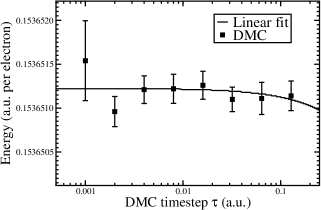
Figure 1: DMC energy of the infinitely-thin wire for several different timesteps and a linear fit to the data. The plot is for $r_{s}=1$ a.u. and $N=37$ with 1000 configurations.

The DMC energy did not change beyond statistical error upon varying the number of walkers between 640 and 2000, so we used $\sim 1000$ walkers in our calculations and assumed that population control bias is negligible. The dependence of the energy upon the DMC timestep $\tau$ was also investigated; Fig. 1 shows that for small $\tau$ the energy is constant. We performed our calculations at a single timestep given by $\tau=0.008\;\!r_{s}^{2}$. This fairly conservative choice was made to ensure that time step bias is entirely negligible. The RMS distance diffused by each electron in a single step was thus slightly less than $r_{s}/10$.

For the infinitely-thin wire, we used simulation cells containing 37, 55, 73, and 99 particles subject to periodic boundary conditions for our calculations of the energy, PCF, and SSF. Our MD calculations for the infinitely-thin wire also used a much larger cell with $N=255$. For the harmonic wire, we used cells with $N=123$, $155$, and occasionally $255$ for the $\zeta=1$ systems and cells with $N=22$ and $102$ for the $\zeta=0$ systems.

Previous work encountered difficulties in sampling different spin configurations of the harmonic wire for $\zeta\neq 1$ due to the presence of “pseudonodes” at the antiparallel coalescence points,Malatesta_2000 although these problems were largely overcome by the use of lattice-regularized diffusion Monte Carlo (LRDMC) in Ref. Casula_2006, . The problem occurred because for strong, repulsive interactions the wave function can become small when two antiparallel spins approach one another. Combined with a small time step this can lead to simulations where opposite spins exchange positions infrequently and the space of spin configurations is explored very inefficiently. Use of a small time step is a necessary part of the algorithm of projector methods like DMC. We have avoided ergodicity problems by using VMC to study the harmonic wire; in the VMC method there is no restriction other than ergodicity on the transition probability density and one may propose moves however one wishes provided that the acceptance probability is modified accordingly. We use electron-by-electron sampling with the transition probability density given by a Gaussian centered on the initial electron position. The VMC “time step” in fact bears no relation to real time and is simply the variance of the transition probability density. In practice, the unmodified time steps (chosen to achieve a $50\%$ acceptance ratio) used in VMC are usually large enough to eliminate ergodicity problems, although we found some cases where it was necessary to enforce a lower limit on the width of the transition probability density. Table 1 shows the frequency with which electrons changed positions in our simulations for both high and low density systems with strong and weak confinement.

$r_{s}$ (a.u.)	$b$ (a.u.)	$s_{\rm exch}$
1	0.1	0.051(1)
1	4	0.160(2)
15	0.1	0.0016(2)
15	4	0.0020(3)

Table 1: Frequency with which electrons’ paths cross in our VMC simulations of the harmonic wire. The quantity $s_{\rm exch}$ is the proportion of proposed single-electron moves that result in a change in the ordering of the particles. A typical calculation comprises between $10^{7}$ and $10^{8}$ proposed single-electron moves. The data shown are for $N=22$.

IV Results

IV.1 Energies

$r_{s}$ (a.u.)	$N$	$E_{\rm DMC}$ (a.u. / elec.)
1	37	$0$.	$1536513(3)$
1	55	$0$.	$1539427(2)$
1	73	$0$.	$1540497(3)$
1	99	$0$.	$1541147(2)$
2	37	$-0$.	$20637509(9)$
2	55	$-0$.	$20628042(7)$
2	73	$-0$.	$20624573(6)$
2	99	$-0$.	$20622457(9)$
5	37	$-0$.	$20397386(3)$
5	55	$-0$.	$20395138(2)$
5	73	$-0$.	$20394308(2)$
5	99	$-0$.	$20393799(2)$
10	37	$-0$.	$14288342(1)$
10	55	$-0$.	$14287568(1)$
10	73	$-0$.	$14287284(1)$
10	99	$-0$.	$142871058(9)$
15	37	$-0$.	$110474492(5)$
15	55	$-0$.	$110470307(4)$
15	73	$-0$.	$110468755(4)$
15	99	$-0$.	$110467811(5)$
20	37	$-0$.	$090782764(5)$
20	55	$-0$.	$090780068(2)$
20	73	$-0$.	$090779064(2)$
20	99	$-0$.	$090778454(2)$

Table 2: The DMC energies for the infinitely-thin wire.

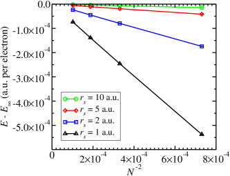
Figure 2: (Color online) Plot of the DMC energy against the reciprocal of the square of the system size for the infinitely-thin wire. The energy has been offset by the extrapolate $E_{\infty}$ that one obtains using the form $E(N)=E_{\infty}+BN^{-2}$.

$r_{s}$ (a.u.)	$E_{\infty}$ (a.u. / elec.)
1	0.	1541886(2)
2	$-0$.	20620084(7)
5	$-0$.	20393235(2)
10	$-0$.	142869097(9)
15	$-0$.	110466761(4)
20	$-0$.	090777768(2)

Table 3: The DMC energies for the infinitely-thin wire extrapolated to the thermodynamic limit using the form $E(N)=E_{\infty}+BN^{-2}$.

For the infinitely-thin wire, we used DMC to calculate the exact ground state energy since there is no ergodicity problem. Table 2 shows the DMC energies that we obtained for $r_{s}=1$, 2, 5, 10, 15, and 20 a.u., with $N=37$, 55, 73, and 99 particles. We find that the Fourier transform of the two-body Jastrow factor $u(k)$ takes the form $u(k)\propto 1/k$ as $k\rightarrow 0$, allowing us to estimate the leading-order scaling of the finite-size correction to the kinetic energy.Chiesa_2006 Furthermore, we observe that the static structure factor $S(k)$ goes to zero linearly at $k=0$, allowing calculation of the corresponding correction for the potential energy.Chiesa_2006 Motivated by these results, we use the form $E(N)=E_{\infty}+BN^{-2}$ to extrapolate to the thermodynamic limit. Figure 2 demonstrates that this form fits the data well, and Table 3 shows the extrapolated energies $E_{\infty}$.

The many-body Bloch theorem states that the wave function $\psi_{T}$ satisfiesRajagopal_1995

$$\Psi_{T}(x_{1},\ldots,x_{j}+L,\ldots,x_{N})=e^{ik_{s}L}\Psi_{T}(x_{1},\ldots,x_{N})\;,$$ (5)

where $L$ is the length of the simulation cell and $k_{s}$ is the simulation cell Bloch wave number. Averaging over $k_{s}$ in the irreducible Brillouin zone (“twist averaging”) has been shown to reduce greatly single-particle finite-size effects in two and three dimensions.Ndd_2009 ; Holzmann_2009 ; Twist_averaging In 1D, however, use of a nonzero $k_{s}$ does not result in reoccupation of the orbitals, merely adding $k_{s}^{2}/2$ to the energy per particle and leaving unchanged (or trivially altering) other expectation values. It is easy to show that the average of $k_{s}^{2}/2$ over the Brillouin zone falls off as $O(N^{-2})$ in 1D; hence single-particle finite-size effects simply lead to an additional $O(N^{-2})$ error in the energy per particle, which is removed when we extrapolate to infinite system size.

The trial wave functions in our calculations for the harmonic wire are of sufficient quality that the variational energies we obtain are in statistical agreement with exact results in the literature;Casula_2006 Table 4 shows the comparison.

$r_{s}$ (a.u.)	$E_{\rm VMC}$ (a.u. / elec.)		$E_{\rm LRDMC}$ (a.u. / elec.)
1	0.	0901489(7)	0.	09014(1)
2	$-0$.	1631207(8)	$-0$.	16311(2)
10	$-0$.	1231560(3)	$-0$.	123157(3)
15	$-0$.	0971194(1)	$-0$.	097120(2)
20	$-0$.	0807160(2)	$-0$.	080717(1)

Table 4: Comparison of our VMC energies for the harmonic wire ($b=1$ a.u., $\zeta=1$) with those of Ref. Casula_2006, , calculated using the LRDMC method. For both sets of results the energies were extrapolated to the thermodynamic limit using the functional form $E(N)=E_{\infty}+BN^{-1}+CN^{-2}$, where $E_{\infty}$, $B$, and $C$ are fitting parameters.

IV.2 Pair-correlation function

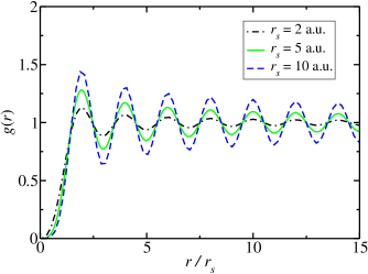
Figure 3: (Color online) PCF of the infinitely-thin wire at several densities. The data shown are for $N=99$ and are extrapolated estimates ${[2g_{\rm DMC}(x)-g_{\rm VMC}(x)]}$.

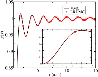
Figure 4: (Color online) PCF of the harmonic wire with $r_{s}=1$ a.u., $N=39$, $b=1$ a.u., and $\zeta=1$. The solid line shows our VMC results and the symbols show the LRDMC results of Ref. Casula_2006, . The inset shows the same data at the origin.

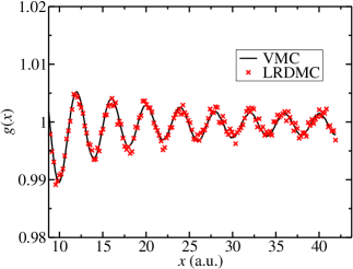
Figure 5: (Color online) PCF of the harmonic wire with $r_{s}=1$ a.u., $N=42$, $b=1$ a.u., and $\zeta=0$. The solid line shows our VMC results and the symbols show the LRDMC results of Ref. Casula_2006, . The function plotted is ${[g_{\uparrow\uparrow}(x)+g_{\uparrow\downarrow}(x)]/2}$.

The PCF is accumulated in QMC simply by binning the interparticle distances throughout the simulation. The parallel-spin PCF is

$$g_{\uparrow\uparrow}(x)=\frac{1}{\rho_{\uparrow}^{2}}\left\langle\sum_{i>j}^{N_{\uparrow}}\delta(|x_{i,\uparrow}-x_{j,\uparrow}|-x)\right\rangle\;,$$ (6)

where $\rho_{\sigma}$ is the average density of electrons with spin $\sigma$, $x_{i,\sigma}$ is the position of the $i$th electron with spin $\sigma$ and the angular brackets denote an average over the configurations generated by the QMC algorithms. The antiparallel-spin PCF may be written as

$$g_{\uparrow\downarrow}(x)=\frac{1}{\rho_{\uparrow}\rho_{\downarrow}}\left\langle\sum_{i}^{N_{\uparrow}}\sum_{j}^{N_{\downarrow}}\delta(|x_{i,\uparrow}-x_{j,\downarrow}|-x)\right\rangle\;.$$ (7)

The PCF for the harmonic wire was calculated for different confinements and system sizes by Casula et al. using the lattice-regularized DMC method.Casula_2006 Figures 4 and 5 show the agreement of the LRDMC results with the present work. Figure 3 shows the PCF for the infinitely-thin wire at several values of $r_{s}$.

IV.3 Static structure factor

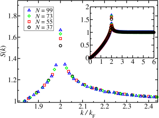
Figure 6: (Color online) SSF of the infinitely-thin wire at several system sizes. The data shown are extrapolated estimates ${[2S_{\rm DMC}(k)-S_{\rm VMC}(k)]}$ for $r_{s}=2\;{\rm a.u.}$. The main plot shows the behavior at the peak and the inset shows a zoomed-out view. The PCF was not extended beyond $L/2$.

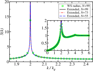
Figure 7: (Color online) Effect of extending the PCF before performing the transformation of Eq. (8). The square symbols (labeled “WS radius”) show the SSF obtained from the finite-cell PCF. The solid, dash-dot, and dashed lines (which all lie on top of one another) are from the $N=99$, $73$, and $55$ PCFs, respectively, where in each case the PCF has been extended out to many simulation cell lengths using the fitting form of Eq. (9). The data shown are for $r_{s}=20$ a.u.

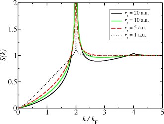
Figure 8: (Color online) SSFs of infinitely thin wires obtained from Eq. (8) and the extended $N=99$ PCFs.

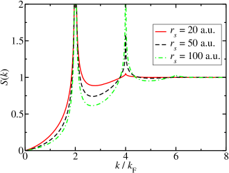
Figure 9: (Color online) SSF of the infinitely-thin wire at very low densities. The results shown are for $N=99$. The finite-cell VMC PCFs were used to generate the SSFs in the plot.

The SSF of the 1D HEG is defined asGiuliani_2005

$$S(k)=1+\frac{N}{L}\int[g(x)-1]e^{-ikx}\;dx\;,$$ (8)

and SSFs that we present here are for the ferromagnetic infinitely-thin wire. As explained in the introduction, the antiferromagnetic and ferromagnetic phases are degenerate for the infinitely-thin wire, so we do not violate the Lieb-Mattis theorem with our choice of system.

The PCF can only be directly measured in QMC for $x<L/2$ due to the finite extent of the simulation cell. This manifests itself as a scaling of the SSF peak at $2k_{\mathrm{F}}$ with system size, as demonstrated by the data in Fig. 6. The height of the $2k_{\mathrm{F}}$ peak in the finite-cell SSFs does not scale as $N$ (and so $L$) to any single power but appears to be sub-linear, consistent with the presence of quasi long-range order. At $k$ away from the peak the SSFs appear to agree very well for different cell sizes.

We further investigated finite-size effects by performing a fit to the oscillatory tails of the PCF and using the fitted function to extend the PCF far beyond $L/2$ before using Eq. (8) to calculate the SSF. After testing a number of functional forms, we found that a good-quality and simple fit to the oscillatory tails of the PCF takes the formCasula_2006 ; Schulz_1993

$$g(x)-1=A\cos(2k_{\mathrm{F}}x)\exp(-B\sqrt{\ln x})\;,$$ (9)

where $A$ and $B$ are treated as fitting parameters. The choice of Eq. (9) is motivated by the charge-charge correlation function of Ref. Schulz_1993, . The parameters we obtained when fitting Eq. (9) to our results are given in Table 5 in Appendix B.

We fitted Eq. (9) to the PCF data for ${6r_{s}<x<L/2-6r_{s}}$, although we found that the results were not very sensitive to the region of data included in the fit. The data close to the origin were not included in the fit since Eq. (9) is only a good fit for long-range correlations. The data at the edge of the cell were excluded because that is the region midway between the electron at the origin and its next periodic image, and might be expected to be a region where the PCF suffers particularly badly from finite-size effects.

We then formed the extended PCF by reinstating all of the original PCF data up to $L/2-6r_{s}$ and appending a tail for $x>L/2-6r_{s}$ using Eq. (9) and the fitted parameters. Performing the Fourier transform of Eq. (8) numerically on the extended PCF results in a SSF (for $r_{s}\leq 20$ a.u.) with a greatly-enhanced peak at $2k_{\mathrm{F}}$, but that agrees very well with the finite-cell SSF everywhere else. Figure 7 shows the difference between the SSFs obtained from the finite-cell and the extended PCFs. Under the extension scheme, the peak at $2k_{\mathrm{F}}$ appears to be susceptible to noise; in particular, the density of $k$-points at which the SSF is calculated heavily affects the apparent height. The fitting function of Eq. (9) possesses a peak at $2k_{\mathrm{F}}$ in Fourier space and smoothly decays away elsewhere, and is expected to be closer to the $N=\infty$ limit.

The asymptotically-correct charge-charge correlation function of SchulzSchulz_1993 includes higher order terms containing oscillations at wave numbers given by even multiples of $k_{\mathrm{F}}$. For $r_{s}<15$ a.u. we find no discernable features at larger $k$. However, a small feature at $4k_{\mathrm{F}}$ starts to develop at $r_{s}\approx 15$ a.u., and for $r_{s}=20$ a.u. we observe a clear peak, visible in Figs. 7, 8, and 9. We performed short VMC calculations at extremely low densities, $r_{s}=50$ a.u. and $100$ a.u., where the electron-electron coupling is very large, to search for more noticeable features at $k>2k_{\mathrm{F}}$. We find that peaks in the SSF do indeed appear at even multiples of $k_{\mathrm{F}}$ for these systems, as evidenced in Fig. 9. The SSF of the $r_{s}=100$ a.u. system has clear peaks at $k=2k_{\mathrm{F}}$, $4k_{\mathrm{F}}$, and $6k_{\mathrm{F}}$. This suggests that one could add higher order terms to the fit of Eq. (9) for the low density systems and perform the extension scheme again, although this seems unlikely to produce any new behavior.

IV.4 Momentum density

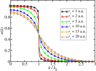
Figure 10: (Color online) MD of the infinitely-thin wire at several densities. The data shown are for $N=99$ and are extrapolated estimates ${[2n_{\rm DMC}(k)-n_{\rm VMC}(k)]}$. The statistical error bars are much smaller than the symbols and some symbols have been omitted for clarity.

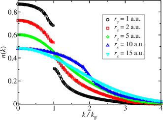
Figure 11: (Color online) VMC MD of the harmonic wire with $b=0.1$ a.u. and $\zeta=0$ at several densities. The data shown for each density are for $N=22$ and $102$ (joined to form one data set). The statistical error bars are smaller than the symbols.

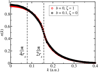
Figure 12: (Color online) Comparison of the $r_{s}=10$ a.u. MD for the infinitely-thin wire ($b=0$, $\zeta=1$) with that obtained for the harmonic wire with $b=0.1$ a.u. and $\zeta=0$. The statistical error bars are similar in size to the symbols. The dashed lines show the values of $k$ at which Eq. (11) was fitted to the data for the calculations of the exponent $\alpha$.

The MD is accumulated as

$$n(k)=\left<\frac{1}{2\pi}\int\frac{\Psi_{\mathrm{T}}(r)}{\Psi_{\mathrm{T}}(x_{1})}\exp[ik(x_{1}-r)]\;dr\right>\;,$$ (10)

where $\Psi_{\mathrm{T}}(r)$ is the trial wave function evaluated at $(r,x_{2},\ldots,x_{n})$ and angular brackets denote an average over configurations. The MD is the integral of the spectral function from minus infinity up to the chemical potential.Giuliani_2005 The MD exhibits a drop at $k_{\mathrm{F}}$ because the peak in the spectral function reaches and passes through the chemical potential. If the peak in the spectral function is a $\delta$-function at $k_{\mathrm{F}}$ (i.e., the spectral function possesses a quasiparticle peak) then the MD is discontinuous at the Fermi edge. However, in 1D we expect the excitations to be collective rather than single-particle-like. The 1D systems should thus have MDs that are continuous at $k_{\mathrm{F}}$, although TL liquid theory predicts that the gradient will be singular.Schulz_1993

For the systems with $\zeta=1$, we have used $k_{\mathrm{F}}=\pi/(2r_{s})$, whereas for the systems with $\zeta=0$, we have used $k_{\mathrm{F}}=\pi/(4r_{s})$. Figure 10 shows the MDs that we obtain by evaluating the extrapolated estimator $2n_{\mathrm{DMC}}(k)-n_{\mathrm{VMC}}(k)$ for the infinitely-thin wire. The VMC and DMC results differed by no more than $\sim 2$ error bars, so that evaluating the extrapolated estimator changed the results very little. Figure 11 shows the MD for the harmonic wire with $b=0.1$ a.u. and $\zeta=0$.

A particularly interesting feature of the paramagnetic harmonic wire MD is that as $r_{s}$ is increased and $b$ is decreased the function shifts much of its weight to larger $k$, and $n(0)$ reduces to values around $0.5$. This is a direct manifestation of the harmonic wire becoming more like the ferromagnetic infinitely-thin system. One can in some cases see a feature resembling the gradient discontinuity appearing at $\pi/(2r_{s})$, i.e., at twice the paramagnetic Fermi wave vector. In particular, for $r_{s}=10$ a.u. and $b=0.1$ a.u. the MD possesses a feature at $\pi/(2r_{s})$. Upon closer inspection we find that the MD for the unpolarized system with $b=0.1$ a.u. agrees very well with that of the infinitely-thin wire ($b=0$ and $\zeta=1$). Figure 12 illustrates this comparison. It thus appears possible to in some sense tune the effective Fermi wave vector by adjusting the strength of the confinement (and the density). A dense paramagnetic system with very weak confinement shows significant occupation of momentum states up to approximately $\pi/(4r_{s})$. Increasing the effective interaction strength increases this value of $k$ until it eventually saturates at the ferromagnetic $k_{F}$. This reflects the fact that in the limit $r_{s}\rightarrow\infty$ the pseudonodes at antiparallel-spin coalescence points become true nodes.

IV.5 Tomonaga-Luttinger liquid parameters

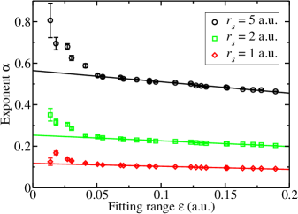
Figure 13: (Color online) Exponent $\alpha$ [found from fitting Eq. (11) to the MD] against the range of data included in the fit. The range of data is described by $|k-k_{\mathrm{F}}|<\varepsilon k_{\mathrm{F}}$. The symbols are the fitted exponent values and the solid lines are linear fits to the exponents in the region $\varepsilon>0.05$. The data shown are for the infinitely-thin wire.

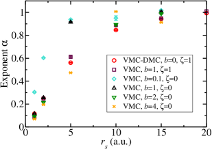
Figure 14: (Color online) Exponent $\alpha$ found from fitting Eq. (11) to the MD around $k=\pi/(2r_{s})$ for the $\zeta=1$ systems and $k=\pi/(4r_{s})$ for the $\zeta=0$ systems.

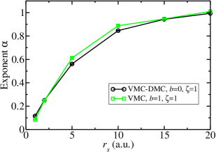
Figure 15: (Color online) Exponent $\alpha$ found from fitting Eq. (11) to the MDs of the ferromagnetic systems.

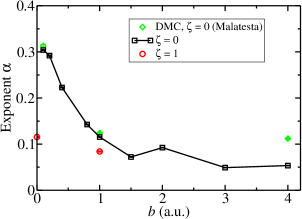
Figure 16: (Color online) Exponent $\alpha$ found from fitting Eq. (11) to the MD of systems with $r_{s}=1$ a.u.

Close to the Fermi wave vector, TL liquid theory suggests that the MD takes the formLuttinger_1963 ; Mattis_1965

$$n(k)=n(k_{\mathrm{F}})+A[{\rm sign}(k-k_{\mathrm{F}})]|k-k_{\mathrm{F}}|^{\alpha}\;,$$ (11)

which we have fitted to our results treating $n(k_{\mathrm{F}})$, $A$, and $\alpha$ as fitting parameters. Note that within TL liquid theory the exponent $\alpha$ is related to the TL liquid parameterSchulz_1990 $K_{\rho}$ by

$$\alpha=\frac{1}{4}\left(K_{\rho}+\frac{1}{K_{\rho}}-2\right)\;.$$ (12)

If the range of data included in the fit is described by $|k-k_{\mathrm{F}}|<\varepsilon k_{\mathrm{F}}$, the choice of $\varepsilon$ can present some difficulties. Ideally, one would choose $\varepsilon\rightarrow 0$ since Eq. (11) is potentially valid for $k\rightarrow k_{\mathrm{F}}$, and indeed using the entire range of MD results yields rather poor fits. However, the estimate of $\alpha$ becomes noisy when $\varepsilon$ is small, and at the extreme where just two data points are included, one can of course obtain any value for $\alpha$. This leads us to include fits constructed using a larger range of $k$ values. In practice, we chose to perform a linear extrapolation to $\varepsilon=0$ excluding fits where $\varepsilon<0.05$ for the $\zeta=1$ systems, as shown in Fig. 13. For the $\zeta=0$ systems, the extrapolation used $\alpha$ from fits for which $\varepsilon\gtrsim 0.25$. The trend that we observe in the exponent with respect to $\varepsilon$ is similar to that found in Ref. Wang_2001, .

Figure 14 shows the exponents $\alpha$ that we obtain for several densities, polarizations, and confinements. All of the systems show the same general trend; $\alpha$ tends to $0$ in the high-density limit and to $1$ in the low-density limit. As mentioned earlier, it is important to note that for the $\zeta=1$ systems we fitted Eq. (11) to the MD at $\pi/(2r_{s})$, whereas for $\zeta=0$ we used $\pi/(4r_{s})$. The change in shape of the MD upon varying the interaction strength that we noted in Sec. IV.4, and the apparent shift in $k_{\mathrm{F}}$, suggests that one could also extract a relevant exponent from fitting to other values of $k$. For example, we showed in Fig. 12 the similarity between the $r_{s}=10$ a.u., $b=0.1$ a.u., $\zeta=0$ MD and that of the $r_{s}=10$ a.u., $b=0$, $\zeta=1$ system. Despite the similarity of the MDs for the two systems, the fits used to extract $\alpha$ from each were performed at different values of $k$ — a factor of two apart in fact. The result is that the exponent for the paramagnetic wire is larger, since the Fermi edge for that system has apparently shifted to $k$ above the fitting region.

With this in mind, Fig. 15 shows the $\zeta=1$ results alone, since for the ferromagnetic systems one can clearly and reliably state that $k_{\mathrm{F}}=\pi/(2r_{s})$ for the whole range of densities. The exponent $\alpha$ for the infinitely-thin wire is reasonably well-approximated by the function

$$\alpha=\tanh(r_{s}/8)\;,$$ (13)

which gives a maximum deviation of $0.011(3)$ from the $b=0$ QMC results, which occurs at $r_{s}=15$ a.u. The exponents for the harmonic wire with $b=1$ a.u. and $\zeta=1$ show a maximum deviation from Eq. (13) of $0.057(6)$, which we find at $r_{s}=5$ a.u.

The exponent $\alpha$ has been reported in previous theoretical and experimental studies. Reference Malatesta_thesis, gives the exponents for $b=0.1$, $1$, and $4$ a.u. (with $r_{s}=1$ a.u. and $\zeta=0$) from VMC calculations. In Fig. 16 we have shown how the results given there compare with ours. It appears that the principal difference between the two studies is the procedure for deciding upon a fitting region; Ref. Malatesta_thesis, does not give details of any extrapolation to $\varepsilon=0$ and presumably the whole range of $n(k)$ was included in the fit. Figure 16 also includes the exponent we find for the infinitely-thin wire (from VMC and DMC estimates of the MD) at $b=0$.

The exponent $\alpha$ has also been reported from experiments, mostly through measurements accessing the single-particle density of states near the Fermi edge. The exponent for carbon nanotubes ranges between $0.2$ and $0.4$, although it is difficult to map the behavior of electrons in these systems onto our model since the electronic properties depend on the folding geometry.Dresselhaus_2001 ; Egger_1998 ; Bockrath_1999 ; Ishii_2003 ; Shiraishi_2003 For the Bechgaard salts, which have a 1D carrier density of $r_{s}\approx 6.9$ a.u., exponents between $0.5625$ and $0.8$ have been reported.Popovic_2001 ; Vescoli_1998 ; Dressel_2005 ; Georges_2000

V Conclusions

We have presented calculations of the ground state energy, PCF, SSF, and MD of the infinitely-thin 1D HEG model using VMC and DMC. We observe the development of peaks at increasingly-large even-integer-multiples of $k_{\mathrm{F}}$ in the SSF as the density is lowered, consistent with the predictions of Schulz.Schulz_1993

For the harmonic wire model, we have reported ground-state MDs and TL parameters for a range of densities and confinements. We used VMC to produce these results; comparison of our PCFs, SSFs, and ground state energies with LRDMC resultsCasula_2006 where available indicates that our results are extremely accurate.

The MDs of the $\zeta=0$ systems tend towards the MDs of the infinitely-thin wire and ferromagnetic harmonic wire as $b$ is decreased and as $r_{s}$ is increased, both of which have the effect of increasing the electron-electron coupling. One interpretation for this is that correlation is dominating over kinetic confinement, so that antiparallel spin pairs are avoiding one another almost as much as parallel spin pairs.

The TL parameters calculated for the $b=1$ a.u., $\zeta=1$ system show reasonable agreement with the infinitely-thin wire results; the maximum deviation that we observe between the parameters for the two systems is $0.051(6)$, which occurs at $r_{s}=5$ a.u. The exponent $\alpha$, which describes the behavior of the MD at $k_{\mathrm{F}}$, takes values between $0$ and $1$. The exponent for the $\zeta=0$ systems shows the same general trend, although the value of $\alpha$ is typically higher than for the $\zeta=1$ systems. This is largely a consequence of the shift of the weight in the MD (including the singularity in the gradient) to larger $k$ as the coupling is increased.

Appendix A Derivation of the quasi-1D interaction

One may derive Eq. (4) from first principles. Suppose the energy scales are such that we may write the wave function as a product $\theta(\boldsymbol{r}_{\perp})\psi(x)$, where $x$ is the projection of the electron position onto the axis of the wire and $\boldsymbol{r}_{\perp}$ is the transverse position.

If the electrons are sufficiently confined in the transverse plane, one may obtain the 1D interaction $v(x)$ by integrating over the transverse part of the wave function,

$$v(x)=\int\frac{|\theta(\boldsymbol{r}_{\perp})|^{2}\;|\theta(\boldsymbol{r}^{\prime}_{\perp})|^{2}}{\big{[}x^{2}+|\boldsymbol{r}_{\perp}-\boldsymbol{r}^{\prime}_{\perp}|^{2}\big{]}^{1/2}}\;d\boldsymbol{r}_{\perp}d\boldsymbol{r}^{\prime}_{\perp}\;.$$ (14)

For the harmonic wire, the confining potential is $r^{2}_{\perp}/8b^{4}$, where $b$ is a parameter. If $r_{s}\gg\pi b/4$, one may make the assumption that the electrons occupy only the lowest sub-band, which is given by

$$\theta(r_{\perp})=\frac{1}{\sqrt{2\pi b^{2}}}\exp\left(-\frac{r_{\perp}^{2}}{4b^{2}}\right)\;.$$ (15)

Substituting Eq. (15) into Eq. (14) yieldsFriesen_1980

$$v(x)=\frac{\sqrt{\pi}}{2b}\exp\left(\frac{x^{2}}{4b^{2}}\right){\rm erfc}\left(\frac{|x|}{2b}\right)\;,$$ (16)

which is finite at $x=0$ but retains a long-range $1/|x|$ tail. The Fourier transform of Eq. (16) is

$$\tilde{v}(k)=E_{1}(b^{2}k^{2})\exp(b^{2}k^{2})\;,$$ (17)

where $E_{1}$ is the exponential integral function.

Having found the real and reciprocal space representations of the 1D interaction in a harmonic wire, one must perform an Ewald-like sum to enable calculations with periodic systems. We follow a route similar to that of Ref. Malatesta_thesis, .

The interaction of an electron at the origin with another at position $x$, all of that electron’s periodic images, and its background is given by

$$\phi(x)=\sum_{m=-\infty}^{\infty}\Big{\{}v(x-mL)-\frac{1}{L}\int^{L/2}_{-L/2}dy\;v(x-mL-y)\Big{\}}\;,$$ (18)

where $L$ is the length of the simulation cell. The objective is to write Eq. (18) in terms of quickly converging discrete sums. The first step is to write Eq. (18) in the more useful form

$$\phi(x)=\gamma_{0}(x)-\frac{1}{L}\int_{-\infty}^{\infty}dy\;v(x-y)\;,$$ (19)

where

$$\gamma_{0}(x)=\sum_{m=-\infty}^{\infty}v(x-mL)\;.$$ (20)

Equation (20) is already in a form that is quick and easy to evaluate, so we turn our attention to reformulating the integral in the second term of Eq. (19). We first perform the trick of both adding and subtracting a Gaussian term $p(y)$, giving

$$-\frac{1}{L}\int_{-\infty}^{\infty}dy\;v(x-y)=\gamma_{1}(x)+\gamma_{2}(x)\;,$$ (21)

where

$$\gamma_{1}(x) = -\int^{\infty}_{-\infty}dy\;v(x-y)p(y)\;,$$ (22)

$$\gamma_{2}(x) = \int^{\infty}_{-\infty}dy\;v(x-y)\left[p(y)-\frac{1}{L}\right]\;,$$ (23)

and the term that we have added and subtracted is

$$p(y)=\sum_{m=-\infty}^{\infty}\frac{1}{2b\sqrt{\pi}}\exp\left(-\frac{1}{4b^{2}}(y-mL)^{2}\right)\;.$$ (24)

It is clear that $\phi(x)$ may now be written simply as

$$\phi(x)=\gamma_{0}(x)+\gamma_{1}(x)+\gamma_{2}(x)\;.$$ (25)

We first inspect $\gamma_{1}(x)$, finding that it may be integrated directly to give

$$\gamma_{1}(x)=\sum_{m=-\infty}^{\infty}\left\{-\frac{1}{|x-mL|}\;{\rm erf}\left(\frac{|x-mL|}{2b}\right)\right\}\;,$$ (26)

which is a form suitable for numerical evaluation.

One may take the first step towards simplifying $\gamma_{2}(x)$ by performing a Poisson summation on $p(y)$,

$$p(y)=\frac{1}{L}\left[1+2\sum^{\infty}_{n=1}e^{-(bGn)^{2}}\cos(Gny)\right]\;,$$ (27)

where $G=2\pi/L$. Putting Eq. (27) into Eq. (23) gives

$$\gamma_{2}(x)=\frac{2}{L}\sum^{\infty}_{n=1}e^{-(bGn)^{2}}\int^{\infty}_{-\infty}dy\;v(x-y)\cos(Gny)\;,$$ (28)

which may straightforwardly be rewritten in its final form,

$$\gamma_{2}(x)=\frac{2\sqrt{2\pi}}{L}\sum_{n=1}^{\infty}\tilde{v}(Gn)\cos(Gnx)\;e^{-(bGn)^{2}}\;,$$ (29)

where we have used the result

$$\int^{\infty}_{-\infty}dy\;v(x-y)\cos(Gny)=\sqrt{2\pi}\;\tilde{v}(Gn)\cos(Gnx)\;.$$ (30)

Finally, putting the expressions for the $\gamma$ functions, Eqs. (20), (26), and (29), into Eq. (25) and remembering that $\tilde{v}(k)$ is given by Eq. (17), we obtain the more computationally convenient form

$$\phi(x) = \sum_{m=-\infty}^{\infty}\Bigg{\{}\frac{\sqrt{\pi}}{2b}e^{(x-mL)^{2}/(4b^{2})}{\rm erfc}\left(\frac{|x-mL|}{2b}\right)$$ (31)

$$- \frac{1}{|x-mL|}\;{\rm erf}\left(\frac{|x-mL|}{2b}\right)\Bigg{\}}$$

$$+ \frac{2}{L}\sum_{n=1}^{\infty}E_{1}\left[(bGn)^{2}\right]\cos(Gnx)\;.$$

It should be noted that in Ref. Casula_2006, , Rydberg rather than Hartree units were used so that the potentials given there differ from Eq. (31) by a factor of 2.

Appendix B Pair correlation function fitting parameters

Table 5 shows the parameters that we obtained when fitting Eq. (9) to the extrapolated estimates of the PCF for the infinitely-thin wire. We performed the fit for $r_{s}=1$, $2$, $5$, $10$, $15$, and $20$ a.u. with systems containing $N=37$, $55$, $73$, and $99$ particles. The PCF data in the range ${6r_{s}<x<L/2-6r_{s}}$ were included in the fit.

$r_{s}$ (a.u.)	$N$	$A$		$B$ (a.u.)
1	37	1.	908	3.	291
1	55	3.	090	3.	683
1	73	1.	940	3.	446
1	99	2.	113	3.	671
2	37	4.	851	2.	952
2	55	4.	573	2.	979
2	73	6.	047	3.	069
2	99	8.	545	3.	273
5	37	8.	029	2.	237
5	55	8.	310	2.	258
5	73	10.	061	2.	359
5	99	9.	262	2.	320
10	37	8.	465	1.	735
10	55	9.	349	1.	788
10	73	9.	066	1.	780
10	99	10.	206	1.	839
15	37	8.	520	1.	502
15	55	8.	363	1.	501
15	73	8.	918	1.	534
15	99	9.	788	1.	580
20	37	7.	754	1.	320
20	55	8.	361	1.	359
20	73	8.	625	1.	377
20	99	8.	895	1.	396

Table 5: Table showing the fitting parameters $A$ and $B$ from Eq. (9) obtained from fitting to the extrapolated estimates of the PCF for the infinitely-thin wire. The fits were to PCF data in the range ${6r_{s}<x<L/2-6r_{s}}$.

References

- (1) G. F. Giuliani and G. Vignale, Quantum Theory of the Electron Liquid (Cambridge University Press, Cambridge, 2005).
- (2) S. Tomonaga, Prog. Theor. Phys. 5, 544 (1950).
- (3) J. M. Luttinger, J. Math. Phys. 4, 1154 (1963).
- (4) F. D. M. Haldane, J. Phys. C: Solid St. Phys. 14, 2585 (1981).
- (5) V. Mitin, A. Sergeev, M. Bell, J. Bird, and A. Verevkin, J. Phys.: Conf. Ser. 193, 012116 (2009).
- (6) M. Bockrath, D. H. Cobden, J. Lu, A. G. Rinzler, R. E. Smalley, L. Balents, and P. L. McEuen, Nature 397, 598 (1999).
- (7) J. Voit, Rep. Prog. Phys. 57, 977 (1994).
- (8) H. J. Schulz, G. Cuniberti, and P. Pieri, arXiv:cond-mat/9807366v2 [cond-mat.str-el] (1998).
- (9) V. Meden, W. Metzner, U. Schollwöck, and K. Schönhammer J. Low Temp. Phys. 126, 1147 (2002).
- (10) T. Ito, A. Chainani, T. Haruna, K. Kanai, T. Yokoya, S. Shin, and R. Kato, Phys. Rev. Lett. 95, 246402 (2005).
- (11) M. Dressel, K. Petukhov, B. Salameh, P. Zornoza, and T. Giamarchi, Phys. Rev. B 71, 075104 (2005).
- (12) T. Lorenz, M. Hofmann, M. Grüninger, A. Freimuth, G. S. Uhrig, M. Dumm, and M. Dressel, Nature 418, 614 (2002).
- (13) A. Schwartz, M. Dressel, G. Grüner, V. Vescoli, L. Degiorgi, and T. Giamarchi, Phys. Rev. B 58, 1261 (1998).
- (14) V. Vescoli, F. Zwick, W. Henderson, L. Degiorgi, M. Grioni, G. Gruner, and L. K. Montgomery, Eur. Phys. J. B 13, 503 (2000).
- (15) M. Dressel, S. Kirchner, P. Hesse, G. Untereiner, M. Dumm, J. Hemberger, A. Loidl, and M. Montgomery, Synth. Met. 120, 719 (2001).
- (16) S. Maekawa, T. Tohyama, S. E. Barnes, S. Ishihara, W. Koshibae, and G. Khaliullin, Physics of Transition Metal Oxides: v. 144, (Springer, 2004).
- (17) Z. Hu, M. Knupfer, M. Kielwein, U. K. Röler, M. S. Golden, J. Fink, F. M. F. de Groot, T. Ito, K. Oka, and G. Kaindl, Eur. Phys. J. B 26, 449 (2002).
- (18) Z. Yao, C. Dekker, and P. Avouris, Electrical Transport Through Single-Wall Carbon Nanotubes, in M. S. Dresselhaus, G. Dresselhaus, and P. Avouris, eds., Carbon Nanotubes: Synthesis, Structure, Properties and Applications (Springer, 2001).
- (19) R. Egger and A. O. Gogolin, Eur. Phys. J. B 3, 281 (1998). nanotubes at low temperatures
- (20) H. Ishii, H. Kataura, H. Shiozawa, H. Yoshioka, H. Otsubo, Y. Takayama, T. Miyahara, S. Suzuki, Y. Achiba, M. Nakatake, T. Narimura, M. Higashiguchi, K. Shimada, H. Namatame, and M. Taniguchi, Nature 426, 540 (2003).
- (21) M. Shiraishi and M. Ata, Sol. State Commun. 127, 215 (2003).
- (22) F. P. Milliken, C. P. Umbach, and R. A. Webb, Sol. State Commun. 97, 309 (1996).
- (23) A. M. Chang, Rev. Mod. Phys. 75, 1449 (2003).
- (24) S. S. Mandal and J. K. Jain, Sol. State Commun. 118, 503 (2001).
- (25) H. Steinberg, O. M. Auslaender, A. Yacoby, J. Qian, G. A. Fiete, Y. Tserkovnyak, B. I. Halperin, K. W. Baldwin, L. N. Pfeiffer, and K. W. West, Phys. Rev. B 73, 113307 (2006).
- (26) S. V. Zaitsev-Zotov, Y. A. Kumzerov, Y. A. Firsov, and P. Monceau, J. Phys.: Condens. Matter 12, L303 (2000).
- (27) F. Liu, M. Bao, K. L. Wang, C. Li, B. Lei, and C. Zhou, Appl. Phys. Lett. 86, 213101 (2005).
- (28) A. R. Goñi, A. Pinczuk, J. S. Weiner, J. M. Calleja, B. S. Dennis, L. N. Pfeiffer, and K. W. West, Phys. Rev. Lett. 67, 3298 (1991).
- (29) ,O. M. Auslaender, A. Yacoby, R. dePicciotto, K. W. Baldwin, L. N. Pfeiffer, and K. W. West, Phys. Rev. Lett. 84, 1764 (2000).
- (30) H. Moritz, T. Stoferle, K. Guenter, M. Kohl, T. Esslinger, Phys. Rev. Lett. 94, 210401 (2005).
- (31) A. Recati, P. O. Fedichev, W. Zwerger, and P. Zoller, J. Opt. B: Quantum Semiclass. Opt. 5 S55 (2003).
- (32) H. Monien, M. Linn, and N. Elstner, Phys. Rev. A 58, R3395 (1998).
- (33) J. Schäfer, C. Blumenstein, S. Meyer, M. Wisniewski, and R. Claessen, Phys. Rev. Lett. 101, 236802 (2008).
- (34) H. J. Schulz, Phys. Rev. Lett. 71, 1864 (1993).
- (35) G. E. Astrakharchik and M. D. Girardeau, arXiv:1101.0103v1 [cond-mat.quant-gas], (2010).
- (36) M. M. Fogler, Phys. Rev. Lett. 94, 056405 (2005).
- (37) C. E. Creffield, W. Häuser, and A. H. MacDonald, Europhys. Lett. 53, 221 (2001).
- (38) M. Fabrizio, A. O. Gogolin, and S. Scheidl, Phys. Rev. Lett. 72, 2235 (1994).
- (39) M. Casula, S. Sorella, and G. Senatore, Phys. Rev. B 74, 245427 (2006).
- (40) L. Shulenburger, M. Casula, G. Senatore, and R. M. Martin, Phys. Rev. B 78, 165303 (2008).
- (41) A. Malatesta and G. Senatore, J. Phys. IV 10, 5 (2000).
- (42) W. I. Friesen and B. Bergersen, J. Phys. C: Solid St. Phys. 13, 6627 (1980).
- (43) L. Calmels, A. Gold, Phys. Rev. B 56, 1762 (1997).
- (44) M. Taş, and M. Tomak, Phys. Rev. B 67 235314 (2003).
- (45) V. Garg, R. K. Moudgil, K. Kumar, and P. K. Ahluwalia, Phys. Rev. B 78, 045406 (2008).
- (46) R. Asgari, Solid State Commun. 141, 563 (2007).
- (47) V. R. Saunders, C. Freyria-Fava, R. Dovesi, and C. Roetti, Comp. Phys. Commun. 84, 156 (1994).
- (48) T. Kato, Comm. Pure Appl. Math. 10, 151 (1957).
- (49) E. Lieb and D. Mattis, Phys. Rev. 125, 164 (1962).
- (50) A. Malatesta, Quantum Monte Carlo study of a model one-dimensional electron gas, PhD Thesis, University of Trieste, Trieste, 1999.
- (51) R. J. Needs, M. D. Towler, N. D. Drummond, and P. López Ríos, J. Phys.: Condens. Matter 22, 023201 (2010).
- (52) W. M. C. Foulkes, L. Mitas, R. J. Needs, and G. Rajagopal, Rev. Mod. Phys. 73, 33 (2001).
- (53) C. J. Umrigar, K. G. Wilson, and J. W. Wilkins, Phys. Rev. Lett. 60, 1719 (1988).
- (54) P. R. C. Kent, R. J. Needs, and G. Rajagopal, Phys. Rev. B 59, 12344 (1999).
- (55) N. D. Drummond and R. J. Needs, Phys. Rev. B 72, 085124 (2005).
- (56) C. J. Umrigar, J. Toulouse, C. Filippi, S. Sorella, and R. G. Hennig, Phys. Rev. Lett. 98, 110201 (2007).
- (57) D. M. Ceperley and B. J. Alder, Phys. Rev. Lett. 45, 566 (1980).
- (58) N. D. Drummond, M. D. Towler, and R. J. Needs, Phys. Rev. B 70, 235119 (2004).
- (59) P. López Ríos, A. Ma, N. D. Drummond, M. D. Towler, and R. J. Needs, Phys. Rev. E 74, 066701 (2006).
- (60) S. Chiesa, D. M. Ceperley, R. M. Martin, and M. Holzmann, Phys. Rev. Lett. 97, 076404 (2006).
- (61) G. Rajagopal, R. J. Needs, A. James, S. D. Kenny, and W. M. C. Foulkes, Phys. Rev. B 51, 10591 (1995).
- (62) N. D. Drummond and R. J. Needs, Phys. Rev. Lett. 102, 126402 (2009).
- (63) M. Holzmann, B. Bernu, V. Olevano, R. M. Martin, and D. M. Ceperley, Phys. Rev. B 79, 041308(R) (2009).
- (64) C. Lin, F. H. Zong, and D. M. Ceperley, Phys. Rev. E 64, 016702 (2001).
- (65) D. C. Mattis and E. H. Lieb, J. Math. Phys. 6, 304 (1965).
- (66) H. J. Schulz, Phys. Rev. Lett. 64, 2831 (1990).
- (67) D. W. Wang, A. J. Millis, and S. Das Sarma, Phys. Rev. B 64, 193307 (2001).
- (68) Z. V. Popovic, V. A. Ivanov, O. P. Khoung, and V. V. Moshchalkov, Synth. Metals 124, 421 (2001).
- (69) V. Vescoli, L. Degiorgi, W. Henderson, G. Grüner, K. P. Starkey, and L. K. Montgomery, Science 281, 1181 (1998).
- (70) A. Georges, T. Giamarchi, and N. Sandler, Phys. Rev. B 61, 16393 (2000).