Representations of Each Number Type that Differ by Scale Factors

Abstract

For each type of number, structures that differ by arbitrary scaling factors and are isomorphic to one another are described. The scaling of number values in one structure, relative to the values in another structure, must be compensated for by scaling of the basic operations and relations (if any) in the structure. The scaling must be such that one structure satisfies the relevant number type axioms if and only if the other structure does.

1 Introduction

Numbers play an essential role in many areas of human endeavor. Starting with the natural numbers, $N$, of arithmetic, one progresses up to integers, $I$, rational numbers, $Ra$, real numbers, $R$, and to complex numbers, $C$. In mathematics and physics, each of these types of numbers is referred to as the natural numbers, the integers, rational numbers, real numbers, and the complex numbers. As is well known, though, ”the” means ”the same up to isomorphism” as there are many isomorphic representations of each type of number.

In this paper, properties of different isomorphic representations of each number type will be investigated. Emphasis is placed on representations of each number type that differ from one another by arbitrary scale factors. Here mathematical properties of these representations will be described. The possibility that these representations for complex numbers may be relevant to physics is described elsewhere [1].

Here the mathematical logical description of a representation, as a structure that satisfies a set of axioms relevant to the type of system being considered [2, 3], is used. For the scaled structures considered here, it will be useful in some cases to separate the notion of representation from that of structure, and consider representations as different views of a structure. This will be noted when needed.

Each structure consists of a base set, one or more basic operations, basic relations (if any), and constants. Any structure containing a base set, basic operations, relations, and constants that are relevant for the number type, and are such that the structure satisfies the relevant axioms is a model of the axioms. As such it is as good a representation of the number type as is any other representation.

The contents of structures for the different types of numbers and the chosen axiom sets are shown below:

• $\overline{N}=\{N,+,\times,<,0,1\}$          Nonnegative elements of a discrete ordered commutative ring with identity [4].

• $\overline{I}=\{I,+,-,\times,<,0,1\}$          Ordered integral domain [5].

• $\overline{Ra}=\{Ra,+,-,\times,\div,<,0,1\}$        Smallest ordered field [6].

• $\overline{R}=\{R,+,-,\times,\div,<,0,1\}$          Complete ordered field [7].

• $\overline{C}=\{C,+,-,\times,\div,^{*},0,1\}$      Algebraically closed field of characteristic $0$ plus axioms for complex conjugation [8, 9].

Here an overline, such as in $\overline{N},$ denotes a structure. No overline, as for $N$, denotes a base set. The complex conjugation operation has been added as a basic operation to $\overline{C}$ as it makes the development much easier. The same holds for the inclusion of the division operation in $\overline{Ra},$ $\overline{R},$ and $\overline{C}.$

For this work, the choice of which axioms are used for each of the number types is not important. For example, an alternate choice for $\overline{N}$ is to use the axioms of arithmetic [10]. In this case $\overline{N}$ is changed by deleting the constant $1$ and adding a successor operation. There are also other axiom choices for the real numbers [11].

The importance of the axioms is that they will be used to show that, for two structures related by a scale factor, one satisfies the axioms if and only if the other does. This is equivalent to showing that one is a structure for a given number type if and only if the other one is a structure for the same number type.

These ideas will be expanded in the following sections. The next section gives a general treatment of fields. This applies to all the number types that satisfy the field axioms (rational, real, complex numbers). However much of the section applies to other numbers also (natural numbers, integers). The following five sections apply the general results to each of the number types. The discussions are mainly limited to properties of the number type that are not included in the description of fields.

Section 8 expands the descriptions of the previous sections by considering $\overline{N},\overline{I},\overline{Ra},\overline{R}$ as substructures of $\overline{C}.$ In this case the scaling factors relating two structures of the same type are complex numbers.

Section 9 concludes the paper with a discussion of some consequences and possible uses of these representations in physics.

2 General Description of Fields

It is useful to describe the results of this work for fields in general. The results can then be applied to the different number types, even those that are not fields. Let $\overline{S}$ be a field structure where

$$\overline{S}=\{S,+,-,\times,\div,0,1\}.$$ (1)

Here $S$ with no overline denotes a base set, $+,-,\times,\div$ denote the basic field operations, and $0,1$ denote constants. Denoting $\overline{S}$ as a field structure implies that $\overline{S}$ is a structure that satisfies the axioms for a field [12].

Let $\overline{S}_{p}$ where

$$\overline{S}_{p}=\{S,+_{p},-_{p},\times_{p},\div_{p},0_{p},1_{p}\}.$$ (2)

be another structure on the same set $S$ that is in $\overline{S}.$ The idea is to require that $\overline{S}_{p}$ is also a field structure on $S$ where the field values of the elements of $S$ in $\overline{S}_{p}$ are scaled by $p,$ relative to the field values in $\overline{S}.$ Here $p$ is a field value in $\overline{S}.$

The goal is to show that this is possible in that one can define $\overline{S}_{p}$ so that $\overline{S}_{p}$ satisfies the field axioms if and only if $\overline{S}$ does. To this end the notion of correspondence is introduced as a relation between the field values of $\overline{S}_{p}$ and $\overline{S}.$ The field value, $a_{p},$ in $\overline{S}_{p}$ is said to correspond to the field value, $pa,$ in $\overline{S}.$ As an example, the identity value, $1_{p},$ in $\overline{S}_{p}$ corresponds to the value $p\times 1=p$ in $\overline{S}.$

This shows that correspondence is distinct from the concept of sameness. $a_{p}$ is the same value in $\overline{S}_{p}$ as $a$ is in $\overline{S}.$ This differs from $pa$ by the factor $p.$ The distinction between correspondence and sameness is present only if $p\neq 1.$ If $p=1$, then the two concepts coincide, and $\overline{S}_{p}$ and $\overline{S}$ are the same structures as far as scaling is concerned.

So far a scaling factor has been introduced that relates field values between $\overline{S}_{p}$ and $\overline{S}.$ This must be compensated for by a scaling of the basic operations in $\overline{S}_{p}$ relative to those of $\overline{S}.$

The correspondences of the basic field operations and values in $\overline{S}_{p}$ to those in $\overline{S}$ are given by,

$$\begin{array}[]{c}a_{p}=pa\\ +_{p}=+,\hskip 28.45274pt-_{p}=-\\ \times_{p}=\frac{\textstyle\times}{\textstyle p},\hskip 28.45274pt\div_{p}=p\div.\end{array}$$ (3)

One can use these scalings to replace the basic operations and constants in $\overline{S}_{p}$ and define $\overline{S}^{p}$ by,

$$\overline{S}^{p}=\{S,+,-,\frac{\times}{p},p\div,0,p\}.$$ (4)

Here the subscript, $p,$ in $\overline{S}_{p},$ Eq. 2 is replaced by $p$ as a superscript to distinguish $\overline{S}^{p}$ from $\overline{S}_{p}.$

Both $\overline{S}^{p}$ and $\overline{S}_{p}$ can be considered as different representations or views of a structure that differs from $\overline{S}$ by a scaling factor, $p$. A useful expression of the relation between $\overline{S}_{p}$ and $\overline{S}^{p}$ is that $\overline{S}^{p}$ is referred to either as a representation of $\overline{S}_{p}$ on $\overline{S},$ or as an explicit representation of $\overline{S}_{p}$ in terms of the operations and element values of $\overline{S}.$

Besides changes in the definitions of the basic operations given in Eq. 3 and distinguishing between correspondence and sameness, scaling introduces another change. This is that one must drop the usual assumption that the elements of the base set, $S,$ have fixed values, independent of structure membership. Here the field values of the elements of $S$, with one exception, depend on the structure containing $S.$ In particular, to say that $a_{p}$ in $\overline{S}_{p}$ corresponds to $pa$ in $\overline{S}$ means that the element of $S$ that has the value $a_{p}$ in $\overline{S}_{p}$ has the value $pa$ in $\overline{S}.$ This is different from the element of $S$ that has the same value, $a,$ in $\overline{S}$ as $a_{p}$ is in $\overline{S}_{p}.$

These relations are shown schematically in Figure 1. The valuations associated with elements in the base set $S$ are shown by lines from $S$ to the structures $\bar{S}$ and $\bar{S}_{p}.$

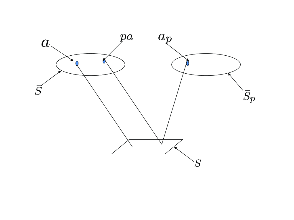
Figure 1: Relations between Elements in the base set $S$ and their Values in the Structures $\bar{S}$ and $\bar{S}_{p}.$ Here $a_{p}$ is the same value in $\bar{S}_{p}$ as $a$ is in $\bar{S}.$ The lines show that they are values for different elements of $S.$ The lines also show that the $S$ element that has the value $a,$ as $a_{p}$ in $\bar{S}_{p}$, has the value $pa$ in $\bar{S}.$

The one exception to the structure dependence of valuations is the element of $S$ with the value $0.$ This value-element association is fixed and is independent of all values of $p.$ In this sense it is the ”number vacuum” as it is invariant under all changes $p\rightarrow p^{\prime}.$

Another approach to understanding the differences between $\overline{S},\overline{S}^{p},$ and $\overline{S}_{p},$ is to distinguish carefully how structure elements are described, when viewed from inside and from outside the structure. Comparison of different structures necessarily is done from outside the structures.

Here there are two structures, $A,B$, with $A$ represented by $\overline{S}$ and $B$ by both $\overline{S}^{p}$ and $\overline{S}_{p}$. There is just one representation, $\overline{S},$ for $A$ because the inside and outside views coincide for this structure. For $A$, correspondence and sameness coincide. In mathematical logical terms the properties of the elements of $A$ are absolute [14]. They are the same when viewed inside or outside the structure. For this reason $\overline{S}$ will often be referred to as a structure instead of a representation.

The situation is quite different for the structure, $B$. Here $\overline{S}^{p}$ and $\overline{S}_{P}$ represent, respectively, external and internal views of $B$. For example, the element of $S$ that has value $p$ in $\overline{S},$ also has value $p$ in $B$ when viewed externally. This shown explicitly in the representation $\overline{S}^{p}.$

When viewed from inside $B$, the element of $S$ that has value $p$ when viewed externally, has the value $1$ when viewed internally or inside $B$. This is designated by the identity $1_{p}$ in $\overline{S}_{p}.$

The situation is somewhat different for the basic operations of multiplication and division. The basic operation of multiplication in $B,$ is shown internally by $\times_{p}$ in $\overline{S}_{p}.$ It is seen externally as the operation $\times/p.$ Here $\times/p=\times(-)\div p$ is the external and internal view of an operation in $A.$ As seen in $\overline{S},$ $\times$ and $\div$ denote the multiplication and division operations in $A.$

One can also define isomorphic maps between the structure representations. Define the maps $W^{p}$ and $W_{p}$ by

$$\overline{S}_{p}=W_{p}\overline{S}^{p}=W_{p}W^{p}\overline{S}=F_{p}\overline{S}.$$ (5)

$W^{p}$ maps $\overline{S}$ onto $\overline{S}^{p}$ and $W_{p}$ maps $\overline{S}^{p}$ onto $\overline{S}_{p}.$ $W^{p}$ is a map from one structure to another, and $W_{p}$ is a map between different representations of the same structure.

$W^{p}$ and $W_{p}$ are defined by

$$\begin{array}[]{c}W^{p}(a)=pa,\\ W^{p}(a\pm b)=W^{p}(a)W^{p}(\pm)W^{p}(b)=(pa)\pm(pb)\\ W^{p}(a\times b)=W^{p}(a)W^{p}(\times)W^{p}(b)=(pa)\frac{\textstyle\times}{\textstyle p}(pb)\\ W^{p}(a\div b)=W^{p}(a)W^{p}(\div)W^{p}(b)=(pa)(p\div)(pb)\end{array}$$ (6)

and

$$\begin{array}[]{c}W_{p}(pa)=a_{p},\\ W_{p}(pa\pm pb)=W_{p}(pa)W_{p}(\pm)W_{p}(pb)=a_{p}\pm_{p}b_{p}\\ W^{p}(pa\frac{\textstyle\times}{\textstyle p}pb)=W^{p}(pa)W^{p}(\frac{\textstyle\times}{\textstyle p})W^{p}(pb)=a_{p}\times_{p}b_{p}\\ W^{p}(pa(p\div)pb)=W^{p}(pa)W^{p}(p\div)W^{p}(pb)=a_{p}\div_{p}b_{p}.\end{array}$$ (7)

It is important to emphasize that the definition of $\overline{S}^{p}$ is not just a relabeling of the elements of $\overline{S}.$ One way to see this is to show that the description of the relations between $\overline{S}^{p}$ and $\overline{S}$ by use of isomorphisms is necessary but not sufficient. To see this let $\overline{S}^{wyz}$ denote a structure where

$$\overline{S}^{wyz}=\{+,-,\frac{\times}{w},(y\div),0,z\}.$$ (8)

Here $w,y,z$ are arbitrary field values in $\overline{S}.$

Define the isomorphism $W^{wyz}:\overline{S}\rightarrow\overline{S}^{wyz}$ by

$$\begin{array}[]{c}W^{wyz}a=za,\hskip 14.22636ptW^{wyz}(\pm)=\pm\\ W^{wyz}(\times)=\frac{\textstyle\times}{\textstyle w},\hskip 14.22636ptW^{wyz}(\div)=y\div.\end{array}$$ (9)

It is clear from the definition of isomorphisms that $\overline{S}^{wyz}$ satisfies the field axioms if and only if $\overline{S}$ does. This follows from the observation that all the field axioms [12] are equations. For example, the existence of a multiplicative identity, $a\times 1=a$ in $\overline{S}$ gives the equivalences

$$\begin{array}[]{l}a\times 1=a\Leftrightarrow W^{wyz}(a)W^{wyz}(\times)W^{wyz}(1)=W^{wyz}(a)\\ \hskip 28.45274pt\Leftrightarrow za\frac{\textstyle\times}{\textstyle w}(z)=za.\end{array}$$ (10)

The righthand equation shows that $z$ is the multiplicative identity in $\overline{S}^{wyz}.$

The equivalences of Eq. 10 show that if one attempts to interpret $\overline{S}^{wyz}$ as an external view of a different structure whose operations and constants are defined in terms of those in $\overline{S}$, then $\overline{S}^{wyz}$ does not represent a field. Requiring that $\overline{S}^{wyz}$ represents a field, limits one to concluding that $\overline{S}^{wyz}$ and $\overline{S}$ represent the same structure. In particular, $\overline{S}^{wyz}$ is just a relabeling of the elements of $\overline{S}$ with no different valuations implied. Note that this limitation is not present for the case where $w=y=z.$

The following two theorems summarize the relations between $\overline{S}^{p},\overline{S}_{p},$ and $\overline{S}.$. The first theorem shows the invariance of equations under the maps, $W^{p}$ and $W_{p}$ where $p,$ is a scaling factor. It also shows, that the correspondence between between element values in $\overline{S}_{p}$ and those in $\overline{S},$ extends to general terms.

Theorem 1

Let $t$ and $u$ be terms in $\overline{S}.$ Let $\overline{S}_{p}$ and $\overline{S}^{p}$ be as defined in Eqs. 2 and 4. Then $t=u\Leftrightarrow t^{p}=u^{p}\Leftrightarrow t_{p}=u_{p}$ where $t^{p}=W^{p}t,$ $u^{p}=W^{p}u,$ and $W_{p}t^{p}=t_{p},W_{p}u^{p}=u_{p}.$

Proof: It follows from the properties of $W^{p}$ and $W_{p},$ Eqs. 6 and 7, that $t^{p}=W^{p}t=pt$ and $u^{p}=W^{p}u=pu.$ Also $t_{p}=W_{p}t^{p}$ and $u_{p}=W_{p}u^{p}.$ This gives

$$t_{p}=u_{p}\Leftrightarrow t^{p}=u^{p}\Leftrightarrow pt=pu\Leftrightarrow t=u.$$ (11)

From the left the first equation is in $\overline{S}_{p}$, the second in $\overline{S}^{p},$ the third in both $\overline{S}^{p}$ and $\overline{S},$ and the fourth in $\overline{S}.$

It remains to see in detail that the correspondence between element values in $\overline{S}_{p}$ and those in $\overline{S}$ extends to terms. Let

$$t_{p}=(\sum_{j,k=1}^{m})_{p}\frac{(a_{p})^{j}}{(b_{p})^{k}}\mbox{}_{p}.$$ (12)

The external view of $t_{p}$ in $\overline{S}^{p}$ is

$$t^{p}=(\sum_{j,k=1}^{m})^{p}\frac{(pa)^{j}}{(pb)^{k}}\mbox{}^{p}.$$ (13)

In the numerator, the $j$ $pa$ factors and $j-1$ multiplications contribute factors of $p^{j}$ and $p^{-j+1},$ respectively, to give a factor $p$. This is canceled by a similar factor arising from the denominator. A final factor of $p$ arises from the representation of the solidus as shown in Eq. 3 for division.

Using this and the fact that addition is not scaled, gives the result that

$$t^{p}=(\sum_{j,k=1}^{m})^{p}\frac{(pa)^{j}}{(pb)^{k}}\mbox{}^{p}=p(\sum_{j,k=1}^{m})\frac{(a)^{j}}{(b)^{k}}\mbox{}=pt.$$ (14)

Eq.11 and the theorem follow from the fact that Eq. 14 holds for any term, including $u^{p}.$ $\blacksquare$

From this one has

Theorem 2

$\overline{S}_{p}$ satisfies the field axioms if and only if $\overline{S}^{p}$ satisfies the field axioms if and only if $\overline{S}$ satisfies the field axioms.

Proof: The theorem follows from Theorem 1 and the fact that all the field axioms are equations for terms. $\blacksquare$

The constructions described here can be iterated. Let $p$ be a number value in $\overline{S}$ and $q\equiv q_{p}$ be a number value in $\overline{S}_{p}.$ Let $\overline{S}_{q|p}$ be another field structure on the base set, $S,$ and let $\overline{S}^{q|p}$ be the representation of $\overline{S}_{q|p}$ using the operations and constants of $\overline{S}_{p}.$ In more detail

$$\overline{S}_{q|p}=\{S,\pm_{q|p},\times_{q|p},\div_{q|p},0,1_{q|p}\}$$ (15)

and

$$\overline{S}^{q|p}=\{S,\pm_{p},\frac{\times_{p}}{q},q\div_{p},0,q1_{p}\}.$$ (16)

$\overline{S}_{q|p}$ is related to $\overline{S}_{p}$ by the scaling factor $q.$ The goal is to determine the scaling factor for the representation of $\overline{S}_{q|p}$ on $\overline{S}.$

To determine this, let $a_{q|p}$ be a value in $\overline{S}_{q|p}.$ This corresponds to a value $q_{p}\times_{p}a_{p}$ in $\overline{S}_{p}.$ Here $a_{q|p}$ is the same value in $\overline{S}_{q|p}$ as $q_{p}\times_{p}a_{p}$ is in $\overline{S}^{q|p}$ as $a_{p}$ is in $\overline{S}_{p}.$

The value in $\overline{S}$ that corresponds to $a_{q|p}$ in $\overline{S}_{q|p}$ can be determined from its correspondent, $q_{p}\times_{p}a_{p},$ in $\overline{S}_{p}.$ The value in $\overline{S}$ that corresponds to $q_{p}\times_{p}a_{p}$ is obtained by use of Eqs. 3 and 7. It is given by

$$(W_{p})^{-1}(q_{p}\times_{p}a_{p})=(pq)\frac{\textstyle\times}{\textstyle p}(pa)=pqa.$$ (17)

Here $q$ and $a$ are the same values in $\overline{S}$ as $q_{p}$ and $a_{p}$ are in $\overline{S}_{p}.$ Also $(W_{p})^{-1},$ as the inverse of $W_{p},$ maps $\overline{S}_{p}$ onto $\overline{S}^{p}.$

This is the desired result because it shows that two steps, first with $p$ and then with $q$ is equivalent to one step with $qp.$ This result shows that the representation of $\overline{S}_{q|p}$ on $\overline{S}$ is given by

$$\overline{S}^{q|p}=\{S,\pm,\frac{\times}{qp},qp\div,0,qp1\}.$$ (18)

Note that the steps commute in that the same result is obtained if one scales first by $q$ and then by $p$ as $pq=qp.$ Here $qp$ is a value in $\overline{S}.$ Also this is equivalent to determining the scale factor for $\overline{S}_{q}$ on $\overline{S}$ provided one accounts for the fact that $q$ is a value in $\overline{S}_{p}$ and not in $\overline{S}.$

3 Natural Numbers

The natural numbers differ from the generic representation in that they are not fields [4]. This is shown by the structure representation for $\overline{N},$

$$\overline{N}=\{N,+,\times,<,0,1\}.$$ (19)

The structure corresponding to $\overline{S}_{n}$ is

$$\overline{N}_{n}=\{N_{n},+_{n},\times_{n},<_{n},0_{n},1_{n}\}.$$ (20)

Here $n$ is any natural number $>0.$

One can use Eq. 3 to represent $\overline{N}_{n}$ in terms of the basic operations, relations, and constants of $\overline{N}.$ It is

$$\overline{N}^{n}=\{N_{n},+,\frac{\times}{n},<,0,n\}.$$ (21)

Note that, as is the case for addition, the order relation is the same in $\overline{N}_{n}$ as in $\overline{N}^{n}$ and in $\overline{N}.$ As was the case for fields, $\overline{N}^{n}$ and $\overline{N}_{n}$ represent external and internal views of a different structure than that represented by $\overline{N}$. For $\overline{N}$ the external and internal views coincide.

The multiplication operator in $\overline{N}^{n},$ $\times/n$ has the requisite properties. This can be seen by the equivalences between multiplication in $\overline{N}_{n},\overline{N}^{n},$ and $\overline{N}:$

$$a_{n}\times_{n}b_{n}=c_{n}\Leftrightarrow na\frac{\times}{n}nb=nc\Leftrightarrow a\times b=c.$$

Note that the simple verification of these equivalences takes place outside the three structures and not within any natural number structure. For this reason division by $n$ can be used to verify the equivalences even though it is not part of any natural number structure.

These equivalences show that $n$ is the multiplicative identity in $\overline{N}^{n}$ if and only if $1$ is the multiplicative identity in $\overline{N}.$ To see this set $b=1.$

The structure, $\overline{N}^{n},$ Eq. 21, and that of Eq. 20, differ from the generic description, Section 2, in that the base set $N_{n}$ is a subset of $N.$ $N_{n}$ contains just those elements of $N$ whose values in $\overline{N}$ are multiples of $n.$ For example, the element with value $n$ in $\overline{N}$ has value $1$ in $\overline{N}_{n},$ and the element with value $na$ in $\overline{N}$ has value $a$ in $\overline{N}_{n}.$ Elements with values $na+l$ in $\overline{N}$ where $0<l<n,$ are absent from $N_{n}.$

As noted before, the choice of the representations of the basic operations and relation and constants in $\overline{N}_{n},$ as shown in $\overline{N}^{n},$ is determined by the requirement that $\overline{N}^{n}$ satisfies the natural number axioms [4] if and only if $\overline{N}$ satisfies the axioms. For the axioms that are equations and do not use the ordering relation, this follows immediately from Theorem 1.

For axioms that use the order relation, the requirement follows from the fact that $<_{n}=<$ and for any pair of terms $t^{n},u^{n}$,

$$t^{n}<_{n}u^{n}\Leftrightarrow nt<nu\Leftrightarrow t<u.$$

Here Eq. 14 was used with $b=1.$ Note that $n>0.$

It follows from these considerations that

Theorem 3

$\overline{N}_{n}$ satisfies the axioms of arithmetic if and only if $\overline{N}^{n}$ does if and only if $\overline{N}$ does.

. A simple example that illustrates the theorem is the axiom of discreteness for the ordering, $0<1\bigwedge\forall a(a>0\rightarrow a\geq 1)$ [4]. One has the equivalences

$$\begin{array}[]{l}0<_{n}1_{n}\bigwedge\forall a_{n}(a_{n}>_{n}0\rightarrow a_{n}\geq_{n}1_{n})\Leftrightarrow 0<n\bigwedge\forall a(na>0\rightarrow na\geq n1)\\ \hskip 28.45274pt\Leftrightarrow 0<1\bigwedge\forall a(a>0\rightarrow a\geq 1).\end{array}$$

Subscripts are missing on $0$ because the value remains the same in all structures.

4 Integers

Integers generalize the natural numbers in that negative numbers are included. Axiomatically they can be characterized as an ordered integral domain [5]. As a structure, $\overline{I}$ is given by

$$\overline{I}=\{I,+,-,\times,<,0,1\}.$$ (22)

$I$ is a base set, $+,-,\times$ are the basic operations, $<$ is an order relation, and $0,1$ are the additive and multiplicative identities.

Let $j$ be a positive integer. Let $\overline{I}_{j}$ be the structure

$$\overline{I}_{j}=\{I_{j},+_{j},-_{j},\times_{j},<_{j},0_{j},1_{j}\}.$$ (23)

$I_{j}$ is the subset of $I$ containing all and only those elements of $I$ whose values in $\overline{I}$ are positive or negative multiples of $j$ or $0.$

The representation of $\overline{I}_{j}$ in terms of elements, operations, and relations in $\overline{I}$ is given by

$$\overline{I}^{j}=\{I_{j},+,-,\frac{\times}{j},<,0,j\}.$$ (24)

This structure differs from that of the natural numbers, Eq. 21, by the presence of the additive inverse, $-.$

The proof that $\overline{I}_{j}$ and $\overline{I}^{j}$ satisfy the integer axioms if and only if $\overline{I}$ does, is similar to that for Theorem 3. The only new operation is the additive inverse. Since the axioms for this are similar to those already present, details of the proof for axioms involving subtraction will be skipped.

A new feature enters in the case that $j$ is negative. It is sufficient to consider the case where $j=-1$ as the case for other negative integers can be described as a combination of $j=-1$ followed by scaling with a positive $j$. This would be done by extending the iteration process, described for fields in Section 2, to integers.

The integer structure representations for $j=-1$ that correspond to Eqs. 23 and 24 are given by

$$\overline{I}_{-1}=\{I,+_{-1},-_{-1},\times_{-1},<_{-1},0_{-1},1_{-1}\},$$ (25)

and

$$\overline{I}^{-1}=\{I,+,-,\frac{\times}{-1},>,0,-1\}.$$ (26)

The main thing to note here is that the order relation, $<_{-1},$ in $\overline{I}_{-1}$ corresponds to $>$ in $\overline{I}.$

$\overline{I}^{-1}$ can also be described as a reflection of the whole structure, $\overline{I}=\overline{I}_{1}$ through the origin at $0.$ Not only are the integer values reflected but also the basic operations and order relation are reflected. Also in this case the base set, $I_{-1}$ =$I.$

Eq. 26 indicates that $-1$ is the identity and $-1$ is positive in $\overline{I}^{-1}.$ These follow from

$$a_{-1}\times_{-1}1_{-1}=a_{-1}\Leftrightarrow(-a)\frac{\times}{-1}(-1)=-a$$

and

$$0<_{-1}1_{-1}\Leftrightarrow 0>-1.$$

This equivalence shows that the relation, $>$, which is interpreted as greater than in $\overline{I},$ is interpreted as less than in $\overline{I}^{-1}.$ Thus, as a relation in $\overline{I}^{-1},$ $0>-1$ means $-1$ is greater than $0.$ As a relation in $\overline{I}$, $0>-1$ means $-1$ is less than $0.$

This is an illustration of the relation of the ordering relation $<_{-1}$ to $<.$ Integers which are positive in $\overline{I}_{-1}$ and $\overline{I}^{-1},$ are negative in $\overline{I}.$ It follows that $0<_{-1}1_{-1}<_{-1}2_{-1}<_{-1}\cdots$ is true in $\overline{I}_{-1}$ if and only if $0>-1>-2>\cdots$ is true in $\overline{I}^{-1}$ and in $\overline{I}.$

These considerations show that $\overline{I}_{-1}$ and $\overline{I}^{-1}$ satisfy the integer axioms if and only if $\overline{I}$ satisfies the axioms. For axioms not involving the order relation the proof is similar to that for $\overline{I}_{j}$ for $j>0.$ For axioms involving the order relation the proofs proceed by restating axioms for $\overline{I}$ in terms of $>.$

An example is the axiom for transitivity $a<b\bigwedge b<c\Rightarrow a<c.$ For this axiom the validity of the equivalence

$$\begin{array}[]{l}(a_{-1}<_{-1}b_{-1}\bigwedge b_{-1}<_{-1}c_{-1}\Rightarrow a_{-1}<_{-1}c_{-1})\\ \hskip 28.45274pt\Leftrightarrow(-a>-b\bigwedge-b>-c\Rightarrow-a>-c)\end{array}$$

shows that this axiom is true in $\overline{I}_{-1}$ if and only if it is true in $\overline{I}^{-1}$ if and only if it is true in $\overline{I}.$

These considerations are sufficient to show that a theorem equivalent to Theorem 3 holds for integers:

Theorem 4

For any integer $j\neq 0$, $\overline{I}_{j}$ satisfies the integer axioms if and only if $\overline{I}^{j}$ does if and only if $\overline{I}$ does.

5 Rational Numbers

The next type of number to consider is that of the rational numbers. Let $\overline{Ra}$ denote a rational number structure

$$\overline{Ra}=\{Ra,+,-,\times,\div,<,0,1\}.$$ (27)

For each positive rational number $r$ let $\overline{Ra}_{r}$ denote the structure

$$\overline{Ra}_{r}=\{Ra,+_{r},-_{r},\times_{r},\div_{r},<_{r},0_{r},1_{r}\}.$$ (28)

Eqs. 27 and 28 show that $\overline{Ra}$ and $\overline{Ra}_{r}$ have the same base set, $Ra.$ This is a consequence of the fact that rational numbers are a field. As such $\overline{Ra}$ nd $\overline{Ra}_{r}$ are special cases of the generic fields described in Section 2. Note also that $\overline{Ra}$ is the same as $\overline{Ra}_{1}.$

The definition of $\overline{Ra}_{r}$ is made specific by the representation of its elements in terms of those of $\overline{Ra}.$ It is

$$\overline{Ra}^{r}=\{Ra,+,-,\frac{\times}{r},r\div,<,0,r\}.$$ (29)

As was seen for fields in Section 2, the number values of the elements of $Ra$ depend on the structure containing $Ra.$ The element of $Ra$ that has value $ra$ in $\overline{Ra}$ has value $a$ in $\overline{Ra}^{r}.$ The element of $Ra$ that has the value $a$ in $\overline{Ra}^{r}$ is different from the element that has the same value $a$ in $\overline{Ra}.$ The only exception is the element with value $0$ as this value is the same for all $\overline{Ra}_{r}.$ Also, as noted in Section 2, $\overline{Ra}^{r}$ and $\overline{Ra}_{r}$ represent external and internal views of a structure that differs from that represented by $\overline{Ra}.$

As was the case for multiplication, the relation between $\div_{r}=r\div$ and $\div$ is fixed by the requirement that $\overline{Ra}_{r}$ satisfy the rational number axioms [6] if and only if $\overline{Ra}^{r}$ satisfies the axioms if and only if $\overline{Ra}$ does. this can be expressed as a theorem:

Theorem 5

Let $r$ be any nonzero rational number. Then $\overline{Ra}$ satisfies the rational number axioms if and only if $\overline{Ra}^{r}$ satisfies the axioms if and only if $\overline{Ra}_{r}$ does.

Proof:
Since the axioms for rational numbers include those of an ordered field, the proof contains a combination of that already given for fields in Section 2, Theorem 1, and for the ordering axioms for integers, as in Theorem 22. As a result it will not be repeated here.

It remains to prove that $\overline{Ra}_{r}$ is the smallest ordered field if and only if $\overline{Ra}^{r}$ is if and only if $\overline{Ra}$ is. To show this, one uses the isomorphisms defined in Section 2.

Let $\overline{S}$ be an ordered field. Let $W^{r}$ and $W_{r}$ be isomorphisms whose definitions on $\overline{Ra}$ and $\overline{Ra}^{r}$ follow that of $W^{p}$ and $W_{p}$ in Eqs. 6 and 7. That is

$$\overline{Ra}_{r}=W_{r}\overline{Ra}^{r}=W_{r}W^{r}\overline{Ra}.$$ (30)

Since these maps, as isomorphisms, are one-one onto and are order preserving, they have inverses which are also isomorphisms. In this case one has

$$\begin{array}[]{l}\overline{Ra}\subseteq\overline{S}\Rightarrow(W^{r})\overline{Ra}=\overline{Ra}^{r}\subseteq\overline{S}\\ \hskip 28.45274pt\Rightarrow(W_{r})\overline{Ra}^{r}=\overline{Ra}_{r}\subseteq\overline{S}\end{array}$$ (31)

and

$$\begin{array}[]{l}\overline{Ra}_{r}\subseteq\overline{S}\Rightarrow(W_{r})^{-1}\overline{Ra}_{r}=\overline{Ra}^{r}\subseteq\overline{S}\\ \hskip 28.45274pt\Rightarrow(W^{r})^{-1}\overline{Ra}^{r}=\overline{Ra}\subseteq\overline{S}.\end{array}$$ (32)

This proves the theorem $\blacksquare.$

For rational number terms, Theorem 1 holds here. From Eq. 13 one sees that for rational number structures,

$$t^{r}=(\sum_{j,k=1}^{m})^{r}\frac{(ra)^{j}}{(rb)^{k}}\mbox{}^{r}=r(\sum_{j,k=1}^{m})\frac{(a)^{j}}{(b)^{k}}\mbox{}=rt.$$ (33)

6 Real Numbers

The description for real numbers is similar to that for the rational numbers. The structures $\overline{Ra}$ and $\overline{Ra}_{r},$ Eqs. 27 and 28, become

$$\overline{R}=\{R,+,-,\times,\div,<,0,1\}$$ (34)

and

$$\overline{R}_{r}=\{R,+_{r},-_{r},\times_{r},\div_{r},<_{r},0_{r},1_{r}\}.$$ (35)

The external representation of the structure, whose internal representation is $\overline{R}_{r},$ is given in terms of the elements, operations, relations and constants of $\overline{R}.$ It is denoted by $\overline{R}^{r}$ where

$$\overline{R}^{r}=\{R,+,-,\frac{\times}{r},r\div,<,0,r\}.$$ (36)

Here $r$ is any positive real number value in $\overline{R}.$. If $r<0$ then $<$ in Eq. 36 is replaced by $>.$

The axioms for the real numbers [7] are similar to those for the rational numbers in that both number types satisfy the axioms for an ordered field. For this reason the proof that $\overline{R}_{r}$ satisfies the ordered field axioms if and only if $\overline{R}^{r}$ satisfies the axioms if and only if $\overline{R}$ does will not be given as it is essentially the same as that for the rational numbers.

Real numbers are required to satisfy an axiom of completeness. For this axiom, let $\{(a_{r})_{j}\}=\{(a_{r})_{j}:j=0,1,2,\cdots\}$ be a sequence of real numbers in $\overline{R}_{r},$ Eq. 35. Let $r$ be a positive real number value in $\overline{R}$. $\{(a_{r})_{j}\}$ converges in $\overline{R}_{r}$ if

$$\begin{array}[]{c}\mbox{For all $\epsilon_{r}>_{r}0$ there exists an $h$ such that }\mbox{for all $j,m>h$}\\ \hskip 28.45274pt|(a_{r})_{j}-_{r}(a_{r})_{m}|_{r}<_{r}\epsilon_{r}.\end{array}$$ (37)

Here $|(a_{r})_{j}-_{r}(a_{r})_{m}|_{r}$ denotes the absolute value, in $\overline{R}_{r},$ of the difference between $(a_{r})_{j}$ and $(a_{r})_{m}.$

The numerical value in $\overline{R}^{r},$ Eq. 36, that is the same as $|(a_{r})_{j}-_{r}(a_{r})_{m}|_{r}$ is in $\overline{R}_{r},$ is given by $|ra_{j}-ra_{m}|.$ This is the same value as $|a_{j}-a_{m}|$ is in $\overline{R}.$ $|ra_{j}-ra_{m}|$ also corresponds to a number value in $\overline{R}$ given by

$$|ra_{j}-ra_{m}|=r|a_{j}-a_{m}|.$$ (38)

Theorem 6

Let $r\neq 0$ be a real number value in $\overline{R}.$ The sequence $\{(a_{r})_{j}\}$ converges in $\overline{R}_{r}$ if and only if $\{ra_{j}\}$ converges in $\overline{R}^{r}$ if and only if $\{a_{j}\}$ converges in $\overline{R}.$

Proof:
     The proof is in two parts: first $r>0,$ and then $r<0.$

$r>0:$ Let $\epsilon_{r}$ be a positive number value in $\overline{R}_{r}$ such that $|(a_{r})_{j}-_{r}(a_{r})_{m}|_{r}<_{r}\epsilon_{r}.$ It follows that $|ra_{j}-ra_{m}|<r\epsilon$ in both $\overline{R}^{r}$ and $\overline{R}.$ Eq. 38 gives the result that $|a_{j}-a_{m}|<\epsilon$ in $\overline{R}.$

Conversely Let $|a_{j}-a_{m}|<\epsilon$ be true in $\overline{R}.$ Then $|ra_{j}-ra_{m}|<r\epsilon$ is true in both $\overline{R}$ and $\overline{R}^{r},$ and $|(a_{r})_{j}-_{r}(a_{r})_{m}|_{r}<_{r}\epsilon_{r}$ is true in $\overline{R}_{r}.$ From this one has the equivalences,

$$|(a_{r})_{j}-_{r}(a_{r})_{m}|_{r}<_{r}\epsilon_{r}\Leftrightarrow r|a_{j}-a_{m}|<r\epsilon\Leftrightarrow|a_{j}-a_{m}|<\epsilon.$$

It follows that $\{(a_{r})_{j}\}$ converges in $\overline{R}_{r}$ if and only if $\{ra_{j}\}$ converges in $\overline{R}^{r}$ if and only if $\{a_{j}\}$ converges in $\overline{R}.$

$r<0$: It is sufficient to set $r=-1.$ In this case $\overline{R}_{-1}$ and $\overline{R}^{-1}$ are given by Eqs. 35 and 36 with $r=-1.$ In this case

$$\overline{R}_{-1}=\{R,+_{-1},-_{-1},\times_{-1},\div_{-1},<_{-1},0_{-1},1_{-1}\}$$ (39)

and

$$\overline{R}^{-1}=\{R,+,-,\frac{\times}{-1},-1\div,>,0,-1\}.$$ (40)

As was the case for integers, and is the case for rational numbers, this structure can also be considered as a reflection of the structure, $\overline{R},$ through the origin at $0.$

As before let $\{(a_{-1})_{j}\}$ be a convergent sequence in $\overline{R}_{-1},$ Eq. 39. The statement of convergence is given by Eq. 37 where $r=-1.$ The statement $|(a_{-1})_{j}-_{-1}(a_{-1})_{m}|_{-1}<_{-1}\epsilon_{-1}$ says that $|(a_{-1})_{j}-_{-1}(a_{-1})_{m}|_{-1}$ is a positive number in $\overline{R}_{-1}$ that is less than the positive number $\epsilon_{-1}$ and $\geq 0.$

The corresponding statement in $\overline{R}^{-1},$ Eq. 40, is

$$|-a_{j}-(-a_{m})|^{-1}>-\epsilon.$$ (41)

Since $\overline{R}^{-1}$ is a reflection of $\overline{R}$ about the origin, the absolute value, $|-|,$ in $\overline{R}$ becomes $r|x|=-|x|$ in $\overline{R}^{-1}.$ In $\overline{R}^{-1},$ the absolute value, $|-|^{-1},$ is always positive even though it is always negative in $\overline{R}.$ For example, $|-a_{j}-(-a_{m})|^{-1}=-|a_{j}-a_{m}|$ where $|-|^{-1}=-|-|$ and $|-|$ are the respective absolute values in $\overline{R}^{-1}$ and $\overline{R}.$

In this case Eq. 41 can be recast as

$$-|a_{j}-a_{m}|>-\epsilon.$$ (42)

This can be used as the convergence condition in Eq. 37. Note that $0\geq-|a_{j}-a_{m}|$ and that $\geq$ denotes ”less than or equal to” in $\overline{R}^{-1}.$

It follows from this that for $r=-1$ that the sequence $\{(a_{-1})_{j}\}$ converges in $\overline{R}_{-1},$ Eq, 39, if and only if the sequence $\{-a_{j}\}$ converges in $\overline{R}^{-1},$ Eq. 40, if and only if the sequence $\{a_{j}\}$ converges in $\overline{R}.$

Extension to arbitrary negative $r$ can be done in two steps. One first carries out the reflection with $r=-1$. This is followed by a scaling with a positive value of $r$ as has already been described in Section 2. $\blacksquare$

Theorem 7

$\overline{R}_{r}$ is complete if and only if $\overline{R}^{r}$ is complete if and only if $\overline{R}$ is complete.

. Proof: Assume that $\overline{R}_{r}$ is complete and that the sequence $\{(a_{r})_{j}\}$ converges in $\overline{R}_{r}$. Then there is a number value $\mu_{r}$ in $\overline{R}_{r}$ such that $\lim_{j\rightarrow\infty}(a_{r})_{j}=\mu_{r}.$ The properties of convergence, Eq. 37, with $(a_{r})_{m}$ replaced by $\mu_{r},$ and Theorem 38, can be used to show that

$$\lim_{j\rightarrow\infty}(a_{r})_{j}=\mu_{r}\Rightarrow\lim_{j\rightarrow\infty}ra_{j}=r\mu\Rightarrow\lim_{j\rightarrow\infty}a_{j}=\mu.$$ (43)

Here $\mu_{r}$ is the same number value in $\overline{R}_{r}$ as $r\mu$ is in $\overline{R}^{r}$ as $\mu$ is in $\overline{R}.$

Conversely assume that $\overline{R}$ is complete and that $\{a_{j}\}$ converges in $\overline{R}$ to a number value $\mu.$ Repeating the above argument gives

$$\lim_{j\rightarrow\infty}(a_{r})_{j}=\mu_{r}\Leftarrow\lim_{j\rightarrow\infty}ra_{j}=r\mu\Leftarrow\lim_{j\rightarrow\infty}a_{j}=\mu.$$ (44)

This shows that $\overline{R}_{r}$ is complete if and only if $\overline{R}^{r}$ is complete if and only if $\overline{R}$ is complete. $\blacksquare$

Since real number structures are fields, Eq. 14 holds for real number terms. That is

$$t^{r}=(\sum_{j,k=1}^{m})^{r}\frac{(ra)^{j}}{(rb)^{k}}\mbox{}^{r}=r(\sum_{j,k=1}^{m})\frac{(a)^{j}}{(b)^{k}}\mbox{}=rt.$$ (45)

These terms can be used to give relations between power series in $\overline{R}_{r},\overline{R}^{r},$ and $\overline{R}.$ Let $P_{r}(n,x_{r})=\sum_{j=1}^{n}(a_{r})_{j}x_{r}^{j}$ be a power series in $\overline{R}_{r}.$ Then $P^{r}(n,rx)$ and $P(n,x)$ are the same power series in $\overline{R}^{r}$ and $\overline{R}$ as $P_{r}(n,x_{r})$ is in $\overline{R}^{r}.$ This means that for each real number value $x_{r},$ $P^{r}(n,rx)$ and $P(n,x)$ are the respective same number values in $\overline{R}^{r}$ and $\overline{R}$ as $P_{r}(n,x_{r})$ is in $\overline{R}_{r}.$ Here $rx$ and $x$ are the same number values in $\overline{R}^{r}$ and $\overline{R}$ as $x_{r}$ is in $\overline{R}_{r}.$

However, the power series in $\overline{R}$ that corresponds to $P_{r}(n,x_{r})$ and $P^{r}(n,rx)$ in $\overline{R}_{r}$ and $\overline{R}^{r}$ is obtained from Eq. 14. It is

$$P_{r}(n,x_{r})=P^{r}(n,rx)=rP(n,x).$$ (46)

This shows that the element of $R$ that has value $P_{r}(n,x_{r})$ in $\overline{R}_{r}$ has value $rP(n,x)$ in $\overline{R}.$

These relations extend to convergent power series. Theorem 38 gives the result that $P_{r}(n,x_{r})$ is convergent in $\overline{R}_{r}$ if and only if $P^{r}(n,rx)$ is convergent in $\overline{R}^{r}$ if and only if $rP(n,x)$ is convergent in $\overline{R}.$ It follows from Theorem 6 and Eqs. 43 and 44 that,

$$\begin{array}[]{l}\lim_{n\rightarrow\infty}P_{r}(n,x_{r})=f_{r}(x_{r})\Leftrightarrow\lim_{n\rightarrow\infty}P^{r}(n,rx)=f^{r}(rx)\\ \hskip 28.45274pt\Leftrightarrow\lim_{n\rightarrow\infty}rP(n,x)=rf(x).\end{array}$$ (47)

Here $f_{r}(x_{r})$ is the same analytic function [15] in $\overline{R}_{r}$ as $f^{r}(rx)$ is in $\overline{R}^{r}$ as $f(x)$ is in $\overline{R}.$

Eqs. 46 and 47 give the result that, for any analytic function $f$ ,

$$f_{r}(x_{r})=f^{r}(rx)=rf(x).$$ (48)

Here $f_{r}$ and $f$ are functions in $\overline{R}_{r}$ and $\overline{R}$ and $f_{r}(x_{r})$ is the same number value in $\overline{R}_{r}$ as $f^{r}(rx)=rf(x)$ is in $\overline{R}^{r}$ as $f(x)$ is in $\overline{R}.$ Simple examples are $e_{r}^{x_{r}}=(e^{r})^{rx}=re^{x}$ for the exponential and $\sin_{r}(x_{r})=sin^{r}(rx)=r\sin(x)$ for the sine function. Caution: $\sin^{2}_{r}(x_{r})=r\sin^{2}(x),$ not $r^{2}\sin^{2}(x).$

7 Complex Numbers

The descriptions of structures for complex numbers is similar to that for the real numbers. Let $\overline{C}$ denote the complex number structure

$$\overline{C}=\{C,+,-,\times,\div,^{*},0,1\}.$$ (49)

For each complex number $c$ let $\overline{C}_{c}$ be the internal representation of another structure where

$$\overline{C}_{c}=\{C,+_{c},-_{c},\times_{c},\div_{c},^{*_{c}},0_{c},1_{c}\}.$$ (50)

The external representation of the structure, in terms of operations and constants in $\overline{C},$ is given by

$$\overline{C}^{c}=\{C,+,-,\frac{\times}{c},c\div,c(-)^{*},0,c1\}.$$ (51)

The relations for the field operations are the same as those for the real numbers except that $c$ replaces $r.$ It follows that Eqs. 45 - 48 hold with $c$ replacing $r.$ These equations show that analytic functions, $f_{c}(x_{c})$ in $\overline{C}_{c},$ have corresponding functions in $\overline{C}$ given by

$$f_{c}(x_{c})=cf(x).$$ (52)

Here $x_{c}$ denotes the same number in $\overline{C}_{c}$ as $x$ is in $\overline{C}.$

The relation for complex conjugation is given by $a_{c}^{*_{c}}=ca^{*}$ It is not $a_{c}^{*_{c}}=c^{*}a^{*}.$ One way to show this is through the requirement that the relation for complex conjugation must be such that $1_{c}$ is a real number value in $\overline{C}_{c}$ if and only if $1$ is a real number value in $\overline{C}.$ This requires that the equivalences

$$1_{c}^{*_{c}}=1_{c}\Leftrightarrow(c1)^{*_{c}}=c1\Leftrightarrow c(1^{*})=c1\Leftrightarrow 1^{*}=1$$

be satisfied. These equivalences show that $(c1)^{*_{c}}=c(1^{*})$ or more generally

$$(a_{c})^{*_{c}}=(ca)^{*_{c}}=c(a^{*}).$$ (53)

Note that any value for $a$ is possible including $c$ or powers of $c.$ For example, $(c_{c}^{n})^{*_{c}}=(c(c^{n}))^{*_{c}}=c(c^{n})^{*}.$

As values of elements of the base set, $C$, Eq. 53 shows that the element of $C$ that has value $a_{c}^{*_{c}}$ in $\overline{C}_{c}$ has value $ca^{*}$ in $\overline{C}.$ This is different from the element of $C$ that has the same value, $a^{*},$ in $\overline{C}$ as $a_{c}^{*_{c}}$ is in $\overline{C}_{c}.$

Another representation of the relation of complex conjugation in $\overline{C}_{c}$ to that in $\overline{C}$ is obtained by writing $c=|c|e^{i\phi}.$ Here $|c|$ is the absolute value of $c.$ This can be used to write

$$(a_{c})^{*_{c}}=(ca)^{*_{c}}=e^{2i\phi}c^{*}a^{*}.$$ (54)

That is $(c-)^{*_{c}}=e^{2i\phi}c^{*}(-)^{*}.$

For most of the axioms, proofs that $\overline{C}_{c}$ satisfies an axiom if and only if $\overline{C}$ does are similar to those for the number types already treated. However, it is worth discussing some of the new axioms. For example the complex conjugation axiom [9] $(x^{*})^{*}=x$ has an easy proof. It is based on Eq. 53, which gives

$$(a_{c}^{*_{c}})^{*_{c}}=((ca)^{*_{c}})^{*_{c}}=(c(a^{*}))^{*_{c}}=c(a^{*})^{*}.$$

From this one has the equivalences,

$$(a_{c}^{*_{c}})^{*_{c}}=a_{c}\Leftrightarrow c(a^{*})^{*}=ca\Leftrightarrow(a^{*})^{*}=a.$$

This shows that $(x^{*})^{*}=x$ is valid for $\overline{C}_{c}$ if and only if it is valid for $\overline{C}^{c}$ and $\overline{C}.$

The other axiom to consider is that for algebraic closure.

Theorem 8

$\overline{C}_{c}$ is algebraically closed if and only if $\overline{C}^{c}$ is algebraically closed if and only if $\overline{C}$ is algebraically closed.

.Proof:
The proof consists in showing that any polynomial equation has a solution in $\overline{C}_{c}$ if and only if the same polynomial equations in $\overline{C}^{c}$ and $\overline{C}$ have the same solutions.

Let $\sum_{j=0}^{n}b_{j}x^{j}=0$ denote a polynomial equation that has a solution $a_{c}$ in $\overline{C}_{c}.$ Then $\sum_{j=0}^{n}(b_{c})_{j}(a_{c})^{j}=0$ in $\overline{C}_{c}.$ Carrying out the replacements $(b_{c})_{j}=cb_{j},$ $a_{c}=ca,$ $\times_{c}=\times/c,$ and $+_{c}=+$ gives the implications

$$\begin{array}[]{l}(\sum_{j=0}^{n})_{c}(b_{c})_{j}(a_{c})^{j}=0\Rightarrow(\sum_{j=0}^{n})^{c}(cb_{j}(ca)^{j})^{c}=0\\ \hskip 28.45274pt\Rightarrow\sum_{j=0}^{n}cb_{j}a^{j}=0\Rightarrow c\sum_{j=0}^{n}b_{j}a^{j}=0\Rightarrow\sum_{j=0}^{n}b_{j}a^{j}=0.\end{array}$$

From the left, the first equation is in $\overline{C}_{c},$ the second is in $\overline{C}^{c}$, and the other three are in $\overline{C}.$ This shows that if $a_{c}$ is the solution of a polynomial in $\overline{C}_{c}$ then $ca$ is the solution of the same polynomial equation in $\overline{C}^{c},$ and $a$ is the solution of the same polynomial equation in $\overline{C}.$

The proof in the other direction consists in assuming that $\sum_{j=0}^{n}b_{j}a^{j}=0$ is valid in $\overline{C}$ for some number $a,$ and reversing the implication directions to obtain $(\sum_{j=0}^{n})_{c}(b_{c})_{j}(a_{c})^{j}=0$ in $\overline{C}_{c}.$ $\blacksquare$

8 Number Types as Substructures of $\overline{C}_{c},$ $\overline{C}^{c},$ and $\overline{C}.$

As is well known each complex number structure contains substructures for the real numbers, the rational numbers, the integers, and the natural numbers. The structures are nested in the sense that each real number structure contains substructures for the rational numbers, the integers, and the natural numbers, etc. Here it is sufficient to limit consideration to the real number substructures of $\overline{C}_{c},$ $\overline{C}^{c},$ and $\overline{C}$.

To this end let $c$ be a complex number and let $\overline{R}_{c}$ and $\overline{R}$ be real number substructures in $\overline{C}_{c}$ and $\overline{C}.$ In this case

$$\overline{R}_{c}=\{R_{c},+_{c},-_{c},\times_{c},\div_{c},<_{c},0_{c},1_{c}\}$$ (55)

and

$$\overline{R}=\{R,+,-,\times,\div,<,0,1\}.$$ (56)

The field operations in $\overline{R}_{c}$ and $\overline{R}$ are the same as those in $\overline{C}_{c}$ and $\overline{C}$ respectively, restricted to the number values of the base sets, $R_{c}$ and $R.$

Expression of the field operations and constants of $\overline{R}_{c}$ in terms of those of $\overline{C}$ gives a representation of $\overline{R}_{c}$ that corresponds to Eq. 51. It is

$$\overline{R}^{c}=\{R_{c},+,-,\frac{\times}{c},c\div,<^{c},0,c1\}.$$ (57)

Recall that the number values associated with the elements of a base set are not fixed but depend on the structure containing them. $R$ contains just those elements of $C$ that have real values in $\overline{C}.$ $R_{c}$ contains just those values of $C$ that that have real values in $\overline{C}^{c}$ and $\overline{C}_{c}.$

Let $x$ be an element of $R$ that has a real value, $a,$ in $\overline{R}.$ This is different from another element, $y,$ of $R_{c}$ that has the same real value, $a_{c},$ in $\overline{R}_{c}$ as $a$ is in $\overline{R}.$ The element, $y,$ also has the value, $ca,$ in $\overline{R}^{c},$ which is the same real value in $\overline{R}^{c}$ as $a$ is in $\overline{R}.$

This shows that $y$ cannot be an element of $R$ if $c$ is complex. The reason is that $ca$ is a complex number value in $\overline{C},$ and $R$ cannot contain any elements of $C$ that have complex values in $\overline{C}.$

It follows that, if $c$ is complex, then $R_{c}$ and $R$ have no elements in common, except for the element with value $0$, which is the same in all structures.

The order relations $<_{c},$ $<^{c},$ and $<$ are defined relations as ordering is not a basic relation for complex numbers. A simple definition of $<$ in $\overline{R}$ is provided by defining $a<b$ in $\overline{C}$ by

$$a<b\left\{\parbox{170.71652pt}{if $a$ and $b$ are real number values in $\overline{C}$ and there exists a positive real number value, $d,$ in $\overline{C}$ such that $a+d=b.$}\right.$$ (58)

Here $d$ is a positive real number in $\overline{C}$ if there exists a number $g$ in $\overline{C}$ such that $d=(g^{*})g.$ The definition for $<_{c}$ in $\overline{R}_{c}$ is obtained by putting $c$ subscripts everywhere in Eq. 58.

The order relation $<^{c}$ in $\overline{R}^{c}$ is

$$ca<^{c}cb\left\{\parbox{170.71652pt}{if $ca$ and $cb$ are real numbers in $\overline{C}^{c},$ and there exists a positive real number $cd$ such that $ca+cd=cb.$}\right.$$ (59)

Here $cd$ is a positive real number in $\overline{C}^{c}$ if there exists a number $cg$ in $\overline{C}^{c}$ such that $cd=(cg)^{*_{c}}cg.$

One still has to prove that these definitions of ordering are equivalent:

Theorem 9

Let $a,$ $b$ be real number values in $\overline{R}.$ Then $a<b\Leftrightarrow ca<^{c}cb\Leftrightarrow a_{c}<_{c}b_{c}.$

Proof:
Replace the three order statements by their definitions, Eqs. 58 and 59, to get $a+d=b\Leftrightarrow ca+cd=cb\Leftrightarrow a_{c}+_{c}d_{c}=b_{c}.$ Here $d=g^{*}g$, $cd=(cg)^{*^{c}}(cg)$, and $d_{c}=g_{c}^{*_{c}}g_{c}.$

Let $a,b,g$ be real numbers values in $\overline{R}.$ Then $ca,cb,cg$ and $a_{c},b_{c},g_{c}$ are the same real number values in $\overline{R}^{c}$ and $\overline{R}_{c}$ as $a,b,g$ are in $\overline{R}.$

Define the positive number value $d$ by $d=g^{*}g.$ Then by Eq. 51, $g^{*}g$ is the same number value in $\overline{R}$ as

$$(cg)^{*_{c}}\frac{\times}{c}(cg)=cg^{*}g=cd$$

is in $\overline{R}^{c}$ as $g_{c}^{*_{c}}g_{c}=d_{c}$ is in $\overline{R}_{c}.$ Thus $cd$ and $d_{c}$ are the same positive number values in $\overline{R}^{c}$ and $\overline{R}_{c}$ as $d$ is in $\overline{R}.$

From this one has

$$a+d=b\Rightarrow ca+cd=cb\Rightarrow a_{c}+_{c}d_{c}=b_{c},$$

which gives

$$a<b\Rightarrow ca<^{c}cb\Rightarrow a_{c}<_{c}b_{c}.$$

The reverse implications are proved by starting with $a_{c},b_{c}$, and $d_{c}=g_{c}^{*_{c}}g_{c}$ and using an argument similar to that given above. $\blacksquare$

9 Discussion

So far the existence of many different isomorphic structure representations of each number type has been shown. Some properties of the different representations, such as the fact that number values, operations, and relations, in one representation are related to values in another representation by scale factors have been described.

Here some additional aspects of these structure representations and their effect on other areas of mathematics will be briefly summarized.

One aspect worth noting is the fact that the rational, real, and complex numbers are a multiplicative group. This can be used to define multiplicative operations on the structures of these three number types and use them to define groups whose elements are the scaled structures.

These are based on maps from the number values to scaled representations. The maps are listed below for each type of number:

• $r\rightarrow\overline{Ra}_{r}\mbox{ $r$ a rational number}$

• $r\rightarrow\overline{R}_{r}\mbox{ $r$ a real number}$

• $c\rightarrow\overline{C}_{c}\mbox{ $c$ a complex number}.$

These maps are restricted to nonzero values of $r,r,c.$

The group properties of the fields for rational, real, and complex numbers, induce corresponding properties in the collection of structures for each of these number types. The discussion will be limited to complex numbers since extension to other number types is similar.

Let $G_{C}$ denote the collection of complex number structures that differ by arbitrary nonzero complex scaling factors. Define the operation, $\diamond$, by

$$\overline{C}_{c}\diamond\overline{C}_{d}=\overline{C}_{cd}.$$ (60)

Justification for this definition is provided by the description of iteration that includes Eqs. 15-18. $G(C)$ is defined relative to the identity group structure, $\overline{C},$ as $c,d$ and $cd$ are values in $\overline{C}.$ Every structure $\overline{C}_{c}$ has an inverse, $\overline{C}_{1/c}$ as

$$\overline{C}_{c}\diamond\overline{C}_{1/c}=\overline{C}.$$ (61)

This shows that $G(C)$ is a group of complex number structures induced by the multiplicative group of complex number values in $\overline{C}.$ Its properties mirror the properties of the group of number values.

Another consequence of the existence of representations of number types that differ by scale factors is that they affect other mathematical systems that are based on different number types as scalars. Examples include any system type that is closed under multiplication by numerical scalars. Specific examples are vector spaces based on either real or complex scalars, and operator algebras.

For vector spaces based on complex scalars, one has for each complex number $c$ a corresponding pair of structures, $\overline{V}_{c},\overline{C}_{c}.$ The scalars for $\overline{V}_{c}$ are number values in $\overline{C}_{c}.$

The representation of $\overline{V}_{c}$ as a structure with the basic operations expressed in terms of those in $\overline{V},$ with $\overline{C}$ as scalars, is similar to that for $\overline{C}_{c},$ Eq. 51. For Hilbert spaces, the structure $\overline{H},$ based on $\overline{C},$ is given by

$$\overline{H}=\{H,+,-,\cdot,\langle-,-\rangle,\psi\}.$$ (62)

Here $\cdot$ and $\langle-,-\rangle$ denote scalar vector multiplication and scalar product. $\psi$ denotes a general state in $\overline{H}.$

The representation of another Hilbert space structure that is based on $\overline{C}_{c},$ is given by

$$\bar{H}_{c}=\{H,+_{c},-_{c},\cdot_{c},\langle-,-\rangle_{c},\psi_{c}\}.$$ (63)

The representation that expresses the basic operations of $\overline{H}_{c}$ in terms of those for $\overline{H}$ is given by

$$\overline{H}^{c}=\{H,+,-,\frac{\textstyle\cdot}{\textstyle c},\frac{\textstyle\langle-,-\rangle}{\textstyle c},c\psi\}.$$ (64)

Details on the derivation of this for the case in which $c$ is a real number are given in [1].

A possible use of these structures in physics is based on an approach to gauge theories [16, 17] in which a finite dimensional vector space $\overline{V}_{x}$ is associated with each space time point $x.$ So far just one complex number field, $\overline{C}$, serves as the scalars for all the $\overline{V}_{x}.$

The possibility of generalizing this approach by replacing $\overline{C}$ with different complex number fields, $\overline{C}_{x}$ at each point $x$ has been explored in [1]. If

$$\bar{C}_{x}=\{C_{x},+_{x},-_{x},\times_{x},\div_{x},\mbox{}^{*_{x}},0_{x},1_{x}\}.$$ (65)

and $y=x+\hat{\nu}dx$ is a neighbor point of $x,$ then the local representation of $\overline{C}_{y}$ at $x$ is given by

$$\bar{C}_{r,x}=\{C_{x},+_{r,x},-_{r,x},\times_{r,x},\div_{r,x},\mbox{}^{*_{r,x}},0_{r,x},1_{r,x}\}.$$ (66)

Number values in $\overline{C}_{r,x}$ are denoted by $a_{r.x}.$

$\overline{C}_{r,x}$ corresponds to $\overline{C}_{c}$, Eq. 50 with $c$ restricted to be a real number. The use of $r$ instead of $c$ was done in [1] to keep the presentation as simple as possible. However it not necessary. Here $r=r_{y,x}$ is a space time dependent real number associated with the link from $x$ to $y.$

The local representation of $\overline{C}_{y}$ on $\overline{C}_{x},$ corresponds to Eq. 51. It is given by

$$\overline{C}^{r}_{x}=\{C_{x},+_{x},-_{x},\frac{\times_{x}}{r},r\div_{x},r(-)^{*_{x}},0_{x},r1_{x}\}.$$ (67)

At point, $x,$ $\overline{C}_{x}$ is the complex number structure that is available to an observer, $O_{x},$ at $x.$ Also $\overline{C}_{y}$ (given by Eq. 65 with $y$ replacing the subscript $x$) is the complex number structure available to $O_{y},$ at point $y.$ The number value, $a_{y},$ is the same value for $O_{y}$ as $a_{x}$ is for $O_{x}.$

However, the value $a_{y}$ at $y$ is seen by $O_{x}$ as an element of $\overline{C}^{r}_{x},$ Eq. 67. This means that $O_{x}$ sees $a_{y}$ as the value $ra_{x}$ in $\overline{C}_{x}.$ Another way to express this is to refer to $ra_{x}$ as the local representation, or correspondent, of $a_{y}$ at $x.$ Then $\overline{C}^{r}_{x}$ is the local representation of $\overline{C}_{y}$ on $\overline{C}_{x}.$ Recall that $ra_{x}=a_{r,x}$ is the same number value in $\overline{C}^{r}_{x}$ and $\overline{C}_{r,x}$ as $a_{x}$ is in $\overline{C}_{x}.$

It is proposed in [1] that this space time dependence of complex number structures may play a role in any theory where a comparison is needed of values of a complex valued function or field $f(x)$ at different space time points. An example is the space time derivative in direction $\hat{\mu}$ of $f:$

$$\partial_{\mu,x}f=\frac{f(x+dx^{\mu})-f(x)}{\partial x^{\mu}}.$$ (68)

The subtraction in Eq. 68 has meaning if and only if both terms are in the same complex number structure, such as $\overline{C}_{x}.$ This is achieved by defining a covariant derivative

$$D_{\mu,x}f=\frac{r_{\mu,x}f(x+dx^{\mu})_{x}-f(x)}{\partial x^{\mu}}.$$ (69)

Here $r_{\mu,x}f(x+dx^{\mu})_{x},$ as a number value in $\overline{C}_{x},$ is the local representation or corresponding value of $f(x+dx^{\mu})$ in $\overline{C}_{x+dx^{\mu}}.$ Also $f(x+dx^{\mu})_{x}$ is the same number value in $\overline{C}_{x}$ as $f(x+dx^{\mu})$ is in $\overline{C}_{x+dx^{\mu}}.$

Gauge fields are introduced by expressing the real number $r_{y,x}$ by

$$r_{y,x}=e^{\vec{A}(x)\cdot\hat{\nu}dx}=e^{\sum_{\mu}A_{\mu}(x)dx^{\mu}}=\prod_{\mu}r_{\mu,x}.$$ (70)

Use of Eqs. 69 and 70 in gauge theory Lagrangians, expanding exponentials to first order in small terms, and keeping terms that are invariant under local gauge transformations, results in $\vec{A}(x)$ appearing as a gauge boson that can have mass (i.e. a mass term is optional in the Lagrangians.)

At present there are no immediate and obvious uses of $\vec{A}(x)$ as a gauge field in physics. It is suspected that $\vec{A}(x)$ may be relevant to some way to relate mathematics and physics at a basic level. As such it might be useful for development of a coherent theory of physics and mathematics together [18, 19]. More work needs to be done to see if these ideas have any merit.

References

• [1] P. Benioff, arXiv 1008.3134.
• [2] J. Barwise, An Introduction to First Order Logic, in Handbook of Mathematical Logic, J. Barwise, Ed. North-Holland Publishing Co. New York, 1977. pp 5-46.
• [3] H. J. Keisler, Fundamentals of Model Theory, in Handbook of Mathematical Logic, J. Barwise, Ed. North-Holland Publishing Co. New York, 1977. pp 47-104.
• [4] R.Kaye, Models of Peano Arithmetic Clarendon Press, Oxford, 1991, pp 16-21.
• [5] Wikipedia:Integral Domain.
• [6] A. J. Weir, Lebesgue Integration and Measure Cambridge University Press, New York, NY, 1973, P. 12.
• [7] J. Randolph, Basic Real and Abstract Analysis, Academic Press, Inc. New York, NY, 1968, P. 26.
• [8] J. Shoenfield, Mathematical Logic, Addison Weseley Publishing Co. Inc. Reading Ma, 1967, p. 86; Wikipedia: Complex Numbers.
• [9] Wikipedia: Complex Conjugate.
• [10] R. Smullyan, GΓΆdel’s Incompleteness Theorems, Oxford University Press,, New York, NY 1992, p. 29; Wikipedia:Peano axioms,
• [11] S. Lang, Algebra 3rd Edition, Addison Weseley Publishing Co. Reading, MA, 1993, p. 272.
• [12] I. Adamson, Introduction to Field Theory, 2nd Edition, Cambridge University Press, New York, NY, 1982, Chapter 1.
• [13] J. Shoenfield,Mathematical Logic, Addison Weseley Publishing Co. Inc., Reading Ma, 1967, p. 79; Wikipedia:L wenheim Skolem theorem
• [14] J. Burgess, Forcing, in Handbook of Mathematical Logic, J. Barwise, Ed. North-Holland Publishing Co. New York, 1977. pp 403-451; W. Hodges, Model Theory, Cambridge University Press, Cambridge, UK, 1993, pp. 47, 150; Wikipedia:absoluteness
• [15] W. Rudin,Principles of Mathematical Analysis 3rd Edition, International series in pure and applied Mathematics McGraw Hill Book Co. New York, NY, 1976, page 172.
• [16] G. Mack, Fortshritte der Physik, 29, 135 (1981).
• [17] I. Montvay and G. MΓΌnster, Quantum Fields on a Lattice, Cambridge Monographs on Mathematical Physics, Cambridge University Press, UK, 1994.
• [18] P. Benioff, Found. Phys., 35, pp 1825-1856, (2005).
• [19] P. Benioff, Found. Phys. 32 pp 989-1029 (2002).