Effective Yukawa couplings and flavor-changing
Higgs boson decays at linear colliders
E. Gabriellia and B. Meleb
a CERN, PH-TH, CH-1211 Geneva 23, Switzerland
b INFN, Sezione di Roma, c/o Dip. di Fisica,
Università di Roma “La Sapienza”,
Piazzale A. Moro 2, I-00185 Rome, Italy
We analyze the advantages of a linear-collider program for testing a recent theoretical proposal where the Higgs-boson Yukawa couplings are radiatively generated, keeping unchanged the standard-model mechanism for electroweak-gauge-symmetry breaking. Fermion masses arise at a large energy scale through an unknown mechanism, and the standard model at the electroweak scale is regarded as an effective field theory. In this scenario, Higgs boson decays into photons and electroweak gauge-boson pairs are considerably enhanced for a light Higgs boson, which makes a signal observation at the LHC straightforward. On the other hand, the clean environment of a linear collider is required to directly probe the radiative fermionic sector of the Higgs boson couplings. Also, we show that the flavor-changing Higgs boson decays are dramatically enhanced with respect to the standard model. In particular, we find a measurable branching ratio in the range for the decay for a Higgs boson lighter than 140 GeV, depending on the high-energy scale where Yukawa couplings vanish. We present a detailed analysis of the Higgs boson production cross sections at linear colliders for interesting decay signatures, as well as branching-ratio correlations for different flavor-conserving/nonconserving fermionic decays.
1 Introduction
The clarification of the electroweak symmetry breaking (EWSB) mechanism is the most urgent task of the Large Hadron Collider (LHC), that last year started taking data at an unprecedented collision energy of TeV. With more collected integrated luminosity and a possible collision energy upgrade, this might soon lead to the long-awaited discovery of the Higgs boson [1]. While the observation and study of the properties of a scalar particle with features not too different from the ones of the standard-model (SM) Higgs boson will be accessible at the LHC, it is well known that a detailed study of the Higgs-boson profile and couplings will crucially benefit from a future linear-collider program [2, 3].
In [4], we introduced a new phenomenological framework giving an improved description of the fermiophobic (FP) Higgs-boson scenario [5]. In particular, we considered the possibility that the Higgs boson gives mass to the electroweak (EW) vector bosons just as in the SM, while fermion masses and chiral-symmetry breaking (ChSB) arise from a different unknown mechanism at an energy scale considerably larger than . Then, the Higgs boson is coupled to the EW vector bosons just as in the SM, while Higgs Yukawa couplings are missing at tree-level in the fermion Lagrangian. Yukawa couplings are anyway generated at one loop after ChSB is introduced by nonstandard explicit fermion mass terms in the Lagrangian. One new energy parameter GeV (the renormalization scale where the renormalized Yukawa couplings vanish) is introduced to give an effective description of the radiative effects of ChSB on Higgs couplings to fermions at low energies. Important logarithmic effects for large values of are resummed via renormalization-group (RG) equations in [4].
Radiative Higgs couplings to fermions turn out in general to be smaller than the corresponding tree-level SM Yukawa couplings. For instance, for GeV, the effective Yukawa coupling to quarks is about 20 to 5 times smaller than the corresponding SM value for GeV to GeV. Nevertheless, the simultaneous reduction in the Higgs boson width, corresponding to the depleted coupling to fermions, considerably compensates for the decrease of the fermionic Higgs decay widths, and gives quite enhanced radiative Higgs branching ratios (BR’s) to fermions. For GeV and GeV, one gets branching ratios to the quarks comparable to the SM values.
In [4], we also discussed the phenomenological expectations at the LHC for the present theoretical framework. Because of the suppression of the Higgs-gluon effective coupling following the absence of the tree-level top-quark Yukawa coupling, the Higgs-boson production at the LHC occurs predominantly by vector-boson fusion (VBF) and associated production (VH) with SM cross sections. For GeV, the decay BR’s for the channels can be enhanced with respect to their SM values by as much as an order of magnitude or more, because of the depleted Higgs total width [4]. As a consequence, in the present scenario, an enhanced two-photon resonance signal in the VBF and production could easily emerge from the background. Indeed, the additional jets (or leptons) in the final states would crucially help in pinpointing the signal events with respect to the SM case, where the dominant production is through . The study of the decay channels at the LHC will give enough information to start to shape up the effective Yukawa scenario with some sensitivity to the scale . On the other hand, the study of the complementary fermion decay channels , that are very challenging at the LHC even in the easier SM case, will require the clean environment of a linear-collider program.
In this paper, we discuss how the excellent potential of a linear collider machine for the precision measurements of the Higgs couplings to fermions could help in testing their radiative structure as predicted in the effective-Yukawa framework. For the first time, beyond the flavor-diagonal couplings, we will go through the flavor-changing (FC) sector of the model, where we find large enhancements with respect to the SM predictions. We will show that studies of the FC Higgs-boson decays at linear colliders can provide extra handles to consolidate the effective Yukawa framework.
The plan of the paper is the following. In Sec. 2, the basic phenomenological features of the effective-Yukawa model are reviewed. In Sec. 3, Higgs-boson production cross sections in collisions at the c.m. energy GeV are presented for different Higgs decay channels. Correlations between the BR’s for the most important fermionic Higgs decays are shown. In Sec. 4, FC Higgs couplings are computed via RG equations. FC decay BR’s are discussed in Sec.5. Our conclusions are presented in Sec. 6.
2 The effective-Yukawa model
In this section, we sum up the main phenomenological features of the effective-Yukawa model, as introduced in [4]***Throughout the paper, for all the basic physical constants and parameters, we assume the same numerical values as in [4]..
In the effective-Yukawa model, EW vector bosons acquire mass via spontaneous symmetry breaking just as in the SM, and a physical Higgs boson is left in the spectrum which is coupled to vector bosons via SM couplings. The peculiar feature of the model is that fermion masses are not assumed to arise from the EW symmetry-breaking mechanism, but from an unknown mechanism at an energy scale considerably larger than . As a consequence, Higgs Yukawa couplings are missing at tree level in the fermion Lagrangian. They are anyway radiatively generated at one-loop after ChSB is introduced by non standard explicit fermion mass terms in the Lagrangian.
In the model, there is just one new free parameter, the energy scale , defined as the renormalization scale where all the Yukawa matrix elements (in flavor space) are assumed to vanish. This renormalization condition just sets the Higgs-fermion decoupling at the high-energy . In particular, we consider in the range GeV. Large logarithmic contributions (where are the SM gauge couplings) to the Yukawa operators are then expected at higher orders in perturbation theory that can be resummed via the standard technique of the RG equations. Notice that the coefficients multiplying these log-terms are universal, that is independent of the structure of the UV completion of the theory. Therefore, they can be calculated in the corresponding effective theory by evaluating the anomalous-dimension matrix of the Yukawa couplings.
As anticipated, while radiative Higgs couplings to fermions in this scenario are smaller than the corresponding SM Yukawa couplings, BR’s for fermionic Higgs decays can be conspicuous for large and GeV. Indeed, the suppression of the fermionic Higgs couplings and of the related fermionic Higgs widths is compensated for by the corresponding depletion in the total Higgs-boson width. In Fig.1, the total Higgs-boson width is shown versus for different values of .
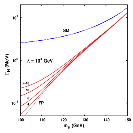
In Fig.1, and in all subsequent plots and tables, the SM and FP labels stand for the standard-model and the naive fermiophobic Higgs scenario results, respectively†††We define as naive fermiophobic Higgs scenario, a model where all the Higgs fermionic couplings are assumed to vanish at the EW scale, and the Higgs boson is coupled to vector bosons as in the SM.. Because of the fall in the light-Higgs total width, values of BR as large as the SM ones can be obtained at high ’s (cf. Table 1, taken from [4]). In particular, for GeV and GeV, one gets BR from radiative effects, to be compared with the corresponding SM values BR.
| BR(%) | BR(%) | BR(%) | BR(%) | BR(%) | BR(%) | BR(%) | ||
| 100 | 12 | 52 | 5.1 | 0.26 | 30 | 0.15 | 0.076 | |
| 8.0 | 33 | 3.3 | 0.17 | 55 | 0.28 | 0.17 | ||
| 4.6 | 19 | 1.9 | 0.094 | 74 | 0.38 | 0.30 | ||
| 3.0 | 12 | 1.2 | 0.062 | 82 | 0.43 | 0.44 | ||
| 100 | FP | 18 | 74 | 7.4 | 0.37 | 0 | 0 | 0 |
| SM | 0.15 | 1.1 | 0.11 | 0.005 | 82 | 3.8 | 8.3 | |
| 110 | 5.3 | 78 | 7.0 | 0.72 | 9.1 | 0.071 | 0.036 | |
| 4.6 | 66 | 5.9 | 0.61 | 22 | 0.18 | 0.11 | ||
| 3.5 | 50 | 4.5 | 0.46 | 41 | 0.33 | 0.26 | ||
| 2.7 | 38 | 3.4 | 0.36 | 54 | 0.45 | 0.45 | ||
| 110 | FP | 5.8 | 86 | 7.7 | 0.79 | 0 | 0 | 0 |
| SM | 0.18 | 4.6 | 0.41 | 0.037 | 78 | 3.6 | 7.9 | |
| 120 | 2.2 | 85 | 9.4 | 0.75 | 2.6 | 0.032 | 0.016 | |
| 2.1 | 81 | 8.9 | 0.72 | 7.5 | 0.092 | 0.056 | ||
| 1.9 | 72 | 8.0 | 0.64 | 17 | 0.21 | 0.16 | ||
| 1.7 | 64 | 7.1 | 0.57 | 26 | 0.32 | 0.33 | ||
| 120 | FP | 2.3 | 87 | 9.7 | 0.77 | 0 | 0 | 0 |
| SM | 0.21 | 13 | 1.5 | 0.11 | 69 | 3.2 | 7.0 | |
| 130 | 1.0 | 86 | 11 | 0.63 | 0.84 | 0.016 | 0.008 | |
| 1.0 | 85 | 11 | 0.62 | 2.6 | 0.048 | 0.029 | ||
| 1.0 | 81 | 11 | 0.59 | 6.1 | 0.12 | 0.092 | ||
| 0.96 | 77 | 10 | 0.57 | 10 | 0.20 | 0.20 | ||
| 130 | FP | 1.0 | 87 | 11 | 0.63 | 0 | 0 | 0 |
| SM | 0.21 | 29 | 3.8 | 0.19 | 54 | 2.5 | 5.4 | |
| 140 | 0.53 | 87 | 12 | 0.48 | 0.29 | 0.008 | 0.004 | |
| 0.53 | 86 | 12 | 0.48 | 0.90 | 0.026 | 0.016 | ||
| 0.53 | 85 | 12 | 0.47 | 2.3 | 0.064 | 0.051 | ||
| 0.52 | 83 | 11 | 0.46 | 4.1 | 0.11 | 0.12 | ||
| 140 | FP | 0.53 | 87 | 12 | 0.48 | 0 | 0 | 0 |
| SM | 0.19 | 48 | 6.6 | 0.24 | 36 | 1.6 | 3.6 |
In Fig.2, the BR’s for the main Higgs-boson decays into vector bosons and photons and fermions are shown versus , for GeV (left) and 140 GeV (right). Also shown is BR() that will be discussed in Sec. 5.
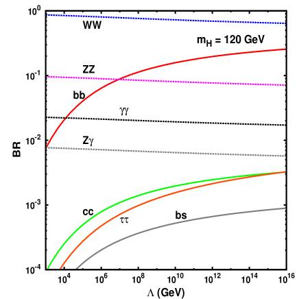
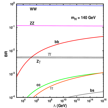
The enhancement of the decays into vector bosons and photons is remarkable (see also plots on the corresponding ratios BR/BRSM in [4]). This is clearly a bonus for Higgs-boson searches at the LHC. On the other hand, all the branching ratios BR() are almost insensitive to the scale . On the contrary, the Higgs decays into fermions, although generally depleted with respect to their SM rates, show a nice sensitivity to , and can provide a handle for a possible determination. To this respect LHC can hardly contribute, while we will discuss in the next section how a linear collider could allow a measurement through the direct detection of Higgs-boson decays into fermions.
Note that neither EW precision tests nor FC neutral current processes presently constrain the effective-Yukawa scenario [4]. Also, the experimental exclusion limits on as elaborated in the SM in direct searches [6, 7] should be revisited in the light of a possible fermionic-coupling depletion that differs from the purely FP limit. A dedicated analysis is needed to obtain bounds in the effective-Yukawa model. A relaxed direct lower bound on is anyway expected with respect to the SM limit of 114.4 GeV [4].
3 Production cross sections for different Higgs boson signatures
It is well-known that, to a great extent, the precision study of light-Higgs-boson properties at linear colliders does not require running at very high c.m. energies [9, 8]. Production cross sections are somewhat optimized for collision energies not much larger than the kinematical threshold for the associated production . While the vector-boson-fusion production rate increases as , and gets comparable to the cross section for (that scales as ) at energies GeV, for lower the associated production has the dominant cross section. In particular, for 120 GeV, pb at GeV, to be compared with the corresponding pb. At GeV, increases and gets dominant, but the total production rate is pb, that is just slightly larger than its value at GeV. The associated production benefits from the further advantage of the simpler two-body kinematics giving rise (at leading order) to a monochromatic Higgs boson, with an excellent potential even in case of an invisible Higgs boson [2].
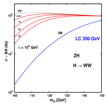
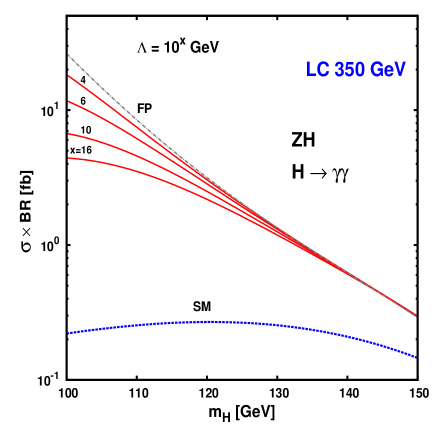
On this basis, we present here the production rates for the dominant Higgs boson decays, for a linear collider running at GeV (that allows top-quark pair production, too). In particular, in Figs. 3–5, we plot the quantities BR versus , for different values of .
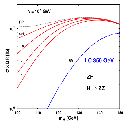
Note that the inclusive Higgs production cross sections are model () independent. Production rates for a different value of and/or for the vector-boson-fusion channel can be obtained from Figs. 3–5 by just rescaling the corresponding cross sections in the SM.
The typical integrated luminosity collected at linear colliders is expected to be a few hundreds of fb-1, and we present in Table 2 the number of expected events corresponding to an integrated luminosity of 500 fb-1 for the production channel , at GeV. Different decay signatures are considered, versus the Higgs boson mass and (both in GeV units). The lower-rate decays and are included in Table 2, too.
| 100 | 9.1 | 3.8 | 3.8 | 1.9 | 2.2 | 1.1 | 5.6 | |
|---|---|---|---|---|---|---|---|---|
| 5.9 | 2.4 | 2.4 | 1.2 | 4.0 | 2.0 | 1.2 | ||
| 3.3 | 1.4 | 1.4 | 6.9 | 5.4 | 2.8 | 2.2 | ||
| 2.2 | 9.0 | 9.0 | 4.5 | 6.0 | 3.2 | 3.2 | ||
| 100 | FP | 1.3 | 5.4 | 5.4 | 2.7 | 0 | 0 | 0 |
| SM | 1.1 | 7.8 | 7.8 | 3.5 | 6.0 | 2.8 | 6.1 | |
| 110 | 3.7 | 5.4 | 4.9 | 5.0 | 6.3 | 4.9 | 2.5 | |
| 3.2 | 4.6 | 4.1 | 4.3 | 1.6 | 1.2 | 7.7 | ||
| 2.4 | 3.5 | 3.1 | 3.2 | 2.9 | 2.3 | 1.8 | ||
| 1.9 | 2.7 | 2.4 | 2.5 | 3.8 | 3.1 | 3.1 | ||
| 110 | FP | 4.1 | 6.0 | 5.4 | 5.5 | 0 | 0 | 0 |
| SM | 1.3 | 3.2 | 2.9 | 2.6 | 5.5 | 2.5 | 5.5 | |
| 120 | 1.5 | 5.6 | 6.2 | 5.0 | 1.7 | 2.1 | 1.1 | |
| 1.4 | 5.3 | 5.9 | 4.7 | 5.0 | 6.1 | 3.7 | ||
| 1.3 | 4.8 | 5.3 | 4.3 | 1.1 | 1.4 | 1.1 | ||
| 1.1 | 4.3 | 4.7 | 3.8 | 1.7 | 2.1 | 2.2 | ||
| 120 | FP | 1.5 | 5.8 | 6.4 | 5.1 | 0 | 0 | 0 |
| SM | 1.4 | 8.9 | 9.9 | 7.0 | 4.6 | 2.1 | 4.6 | |
| 130 | 6.5 | 5.4 | 7.0 | 3.9 | 5.3 | 9.9 | 5.0 | |
| 6.5 | 5.3 | 6.9 | 3.9 | 1.6 | 3.0 | 1.8 | ||
| 6.3 | 5.1 | 6.6 | 3.7 | 3.8 | 7.2 | 5.8 | ||
| 6.0 | 4.8 | 6.3 | 3.5 | 6.5 | 1.2 | 1.2 | ||
| 130 | FP | 6.5 | 5.4 | 7.1 | 4.0 | 0 | 0 | 0 |
| SM | 1.3 | 1.8 | 2.4 | 1.2 | 3.4 | 1.6 | 3.4 | |
| 140 | 3.1 | 5.1 | 6.9 | 2.8 | 1.7 | 4.8 | 2.4 | |
| 3.1 | 5.1 | 6.9 | 2.8 | 5.3 | 1.5 | 9.2 | ||
| 3.1 | 5.0 | 6.8 | 2.8 | 1.3 | 3.8 | 3.0 | ||
| 3.1 | 4.9 | 6.6 | 2.7 | 2.4 | 6.7 | 6.8 | ||
| 140 | FP | 3.1 | 5.1 | 7.0 | 2.8 | 0 | 0 | 0 |
| SM | 1.1 | 2.8 | 3.9 | 1.4 | 2.1 | 9.6 | 2.1 |
Figure 3 shows production rates for (left) and (right). Cross sections are quite enhanced with respect to the SM at low . They are large enough to allow an accurate study of both channels, by exploiting both the leptonic and the hadronic decays. For instance, at GeV, for to GeV, one expects (5.4 to events (to be compared with in the SM), and (4.9 to events (to be compared with in the SM) (cf. Table 2). At lower , the sensitivity to increases, while at larger a determination becomes more and more difficult.
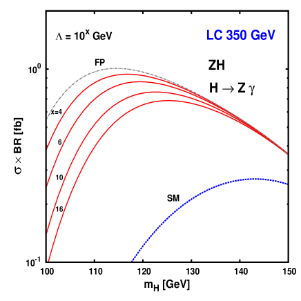
A similar pattern, as far as both rate enhancement and sensitivity to are concerned, is found for the channel [cf. Fig. 4 (left)], that is anyway characterized by a cleaner signature (a resonance). In particular, for GeV, and to GeV, one expects (3.7 to events (to be compared with in the SM) (cf. Table 2). Lower rates are predicted for [cf. Fig. 4 (right)], for which, anyway, a few hundreds of events are expected in most of the parameter space.
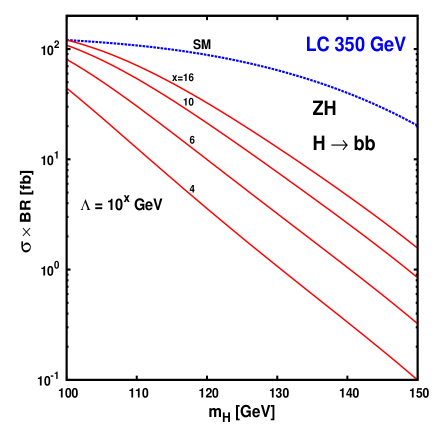
In Fig. 5 (left), the production rates for the decay channel are shown. The channel gives a remarkable opportunity to make an accurate determination in all the range considered here. Not only the rate is quite sensitive to at low , but this sensitivity even increases at high ’s (unlike what occurs for the channels). At GeV, (6.3 to events are predicted (to be compared with in the SM), for to GeV (cf. Table 2). At GeV, the rate is lower but the sensitivity to is much larger. In particular, for to GeV, one expects (1.7 to events (to be compared with in the SM).
The numbers of events corresponding to the channels and are quite suppressed with respect to the SM values. Anyway, the few tens or hundreds of events expected in most of the parameter space (cf. Table 2) should allow a fair BR’s determination for the corresponding decays.
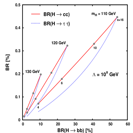
In Fig.5 (right), we show the correlations between the BR’s for the decays and , and BR, for 110, 120, 130 GeV. For each value, is univocally set by BR, and we report the points corresponding to GeV (grey bubbles) only on the curves (related points on the curves can be easily inferred). These correlations are characteristics of the radiative structures of the Yukawa-coupling generation. BR depends linearly on BR, reflecting a similar structure of the corresponding RG equations. Nonlinear differences in the behavior of BR arise from the different impact of strong interactions on the leptonic-coupling evolution with respect to the quark case (see Section 4).
The rates for the different decay channels in Table 2 can give a first hint on how accuracies in the measurement of various Higgs-boson couplings could scale with respect to the corresponding SM values. In previous Higgs-boson studies [2, 10], the expectations for the precision on the Higgs branching ratios and couplings have been reported for linear colliders with GeV and 500 GeV and integrated luminosity of the order of 500 fb-1. A similar precision is then expected for the setup assumed in Table 2. The relative precision on the measurements of the SM branching ratios BR() is a few percent for GeV [2, 10]. The accuracy on BR is a bit lower [2]. In case the effective Yukawa scenario is realized, accuracies on the measurements of BR() will be much better than in the SM. The precision on the measurement of BR will be comparable with the SM estimate at very low , while getting worse in the intermediate and large range. On the other hand, accuracies on BR and especially on BR are expected to deteriorate with respect to the SM case in all the range. A more quantitative analysis would require going into the relevant backgrounds and detection efficiencies.
4 Effective flavor-changing Yukawa couplings
In this section we analyze the flavor-changing (FC) fermionic decays
| (1) |
where the indices stand for generic flavors, in the up-quark (or down-quark) sectors. In the SM, the decay amplitudes for are generated at one loop, and are finite, thanks to the unitarity of the CKM matrix. These decays are characterized by very small BR’s. Even the decay , that is not suppressed by the Glashow-Iliopoulos-Maiani (GIM) mechanism because of the unbalanced top-quark contribution in the loop, has a quite small BR. In particular, for , one has BR [11, 12], which makes this channel practically undetectable in the SM.
On the other hand, the small BR makes the Higgs decay a sensitive probe of potential new physics contributions above the EW scale. This process has been extensively considered in literature, with emphasis on minimal and non-minimal supersymmetric extensions of the SM [12, 13], where the corresponding BR can be as large as () in particular configurations of the allowed SUSY parameter space.
In the following, we will compute BR in the effective Yukawa scenario, and find that it can also be in the range for GeV.
In case a new mechanism for ChSB and generation of fermion masses exists, it is natural to assume that it will generate a fermion mass matrix on the fermion weak eigenstates which is equal to the SM one. The CKM is then obtained as usual by rotating the fermion fields into the fermion mass eigenstates.
Fermion masses explicitly breaking chiral symmetry radiatively induces both flavor-diagonal and flavor-changing Yukawa couplings because of the off-diagonal terms in the CKM matrix. Then for a light Higgs boson one gets a large enhancement in the FC Higgs decay BR’s arising from two combined effects. On the one hand, the Higgs total width is depleted with respect to the SM one, being the -quark Yukawa coupling radiatively generated. On the other hand, there is a significant effect in the resummation of the leading log terms for the FC amplitude for . Moreover, the ratio of the FC decay amplitude for the decay to the flavor-conserving one will not be suppressed by gauge couplings and loop factors as in the SM, but will only be depleted by the CKM matrix element . The same holds for other FC Higgs decays, although an extra suppression by the GIM mechanism will in general affect the ratio. Therefore, a large enhancement in the FC Higgs BRs is naturally expected in our framework.
In order to calculate BR (with ), we start by evaluating the effective flavor-changing Yukawa couplings related to the corresponding interaction term in the Lagrangian. The FC one-loop amplitude is divergent in this scenario, unlike in the SM, since tree-level Yukawa couplings are missing. In the language of effective field theories, this implies that the corresponding FC Yukawa coupling has to be renormalized at some high-energy scale. Then, Yukawa couplings at low energy can be computed by RG equations.
Yukawa couplings, in the fermion mass eigenstates, are defined by the Lagrangians for the flavor-conserving interactions,
| (2) |
where for , , and , respectively, and the FC interactions‡‡‡ In Eq.(3) we have not included the contribution of FC interactions in the charged leptonic sector, that are vanishing in the massless neutrino limit.
| (3) |
where the indices run over the fermion generations, is the Higgs boson field, and, being Hermitian, the matrices satisfy the condition . The diagonal entries of are zero, since the corresponding flavor-conserving contribution is described by the flavor-conserving Yukawa couplings , in Eq.(2). On the other hand, left-handed and right-handed two-fermion operators in Eq.(3) have different radiative couplings whenever initial and final fermions have different masses. From now on, we will neglect CP violating effects in the CKM matrix, and all the Yukawa couplings will be real numbers.
We first recall the RG equations for the flavor-conserving Yukawa couplings , , . In a compact matrix notation, this is given by
| (4) |
where the (diagonal) beta function matrices , with , are [4]
| (5) | |||||
| (6) | |||||
| (7) |
where , , , stands for the trace of the matrix , and is defined as
| (8) |
In particular, (where stand for up-quarks, down-quarks and charged leptons, respectively) are diagonal matrices in flavor space, . Note that the effective Yukawa couplings for leptons enters the effective Yukawa couplings for quarks through Eq. (8). Also,
| (9) |
where is a diagonal matrix in flavor space, being the fermion pole masses, with , and the number of colors. The RG equations for the gauge couplings are the SM ones [14]
| (10) |
with and the number of fermion generations. Terms in give rise to ChSB, and are normalized as the tree-level SM Yukawa couplings. In deriving Eqs.(4)-(7), we neglected subdominant contributions induced by the off-diagonal CKM matrix elements in the charged-current weak corrections. In this approximation, the RG equations for the flavor-diagonal Yukawa couplings do not involve the FC Yukawa couplings.
Now we discuss the RG equations for the FC Yukawa couplings and defined by Eq.(3). Diagrams related to the corresponding functions are shown in Fig. 6,
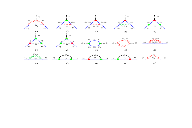
where we have included the full set of EW [Fig.6(a)-6(d), 6(i)-6(k), and 6(o)], strong [Fig.6(d) and 6(k)], and Yukawa [Fig.6(e)-6(h) and 6(l)-6(n)] corrections. In Fig. 6, the green (light) bubbles [in Fig.6(b), 6(e)-6(h), and 6(l)-6(n)] and red (dark) bubbles [in Fig.6(c)-6(g) and 6(m)-6(n)] stand for the vertex insertion of flavor-diagonal and FC Yukawa couplings, respectively. Contributions of double FC vertex insertions have been neglected, as discussed further on.
For vanishing tree-level Yukawa couplings, the leading contribution to the function is given by the diagram in Fig.6(a), where two s are exchanged in the vertex diagram. Indeed, the residue at the pole in diagram in Fig.6(a) is the only contribution to the Yukawa functions which is not proportional to Yukawa couplings. Then, when all Yukawa couplings are set to zero at the energy scale , as required by the condition of Higgs-fermion decoupling, Yukawa couplings are radiatively generated at any energy scale different from (here, in particular, at the scale ) thanks to the diagram in Fig.6(a).
By including the full set of corrections in Fig.(6), we obtain the RG equations for the FC Yukawa couplings§§§ We stress that the RG equations in Eqs. (4)-(7), and (11)-(13) are also valid in a more general scenario in which the Yukawa couplings are not vanishing at tree-level, and are different from their tree-level SM values, provided their tree-level values are small enough not to spoil the perturbative regime.
| (11) |
where the corresponding beta functions , with , are given by
| (12) | |||||
| (13) |
where , , , (with ), are the CKM matrix elements, and the sine of the Weinberg angle. Since , right-handed couplings can simply be obtained from the left-handed ones by the general condition .
In deriving Eqs.(11)-(13), we neglected, in diagram in Fig.6(c), terms of order (with , ), and related fermion self-energies contributions. Indeed, FC couplings (entering the red bubble) are naturally of order in our framework. Then, in the -exchange vertices in Fig.6(c) we kept only diagonal CKM couplings. Consistently, we neglected also contributions coming from double FC vertex insertions.
Notice that in Eqs. (11)-(13), terms that are not proportional to the FC couplings vanish in the SM limit . Indeed, because of the SM renormalizability, the FC interactions in the Higgs sector are finite in the SM, implying that the SM functions for the FC couplings vanish.
In Eqs.(11)-(13), we do not find, as we do in Eqs.(4)-(7), any large term proportional to multiplied by the ChSB factor . Indeed, these terms are in principle generated by the diagram in Fig.6(a), but their total contribution vanishes because of the GIM mechanism and CKM unitarity. On the contrary, the above terms provide the leading contribution to the RG equations for the flavor-diagonal Yukawa couplings Eqs. (4)-(7), and are responsible for the breaking of perturbative unitarity in the Yukawa sector at large [4]. Notice that contributions proportional to in Eqs.(11)-(13) arise from diagrams in Fig.6(c) and corresponding self-energy contributions [diagrams 6(i)-6(j)] to the FC vertex corrections, where the GIM mechanism is not active. On the other hand, they are strongly suppressed by the FC factors, and could endanger perturbative unitarity only for much larger than the range where the flavor-diagonal equations Eqs. (4)-(7) are in the perturbative regime [4].
Following the approach in [4], our renormalization conditions will consist in assuming all the Yukawa couplings vanishing at the scale , namely
Then, the corresponding values at low energy (in particular at ) will be determined by numerically solving the full set of RG equations in Eqs. (4)-(7) and (11)-(13).
| 100 | 1.8 | 8.3 | 2.2 | 2.3 | 1.6 | |
| 3.2 | 1.4 | 3.8 | 3.8 | 2.8 | ||
| 5.1 | 2.2 | 6.0 | 5.8 | 4.3 | ||
| 7.0 | 3.0 | 7.9 | 7.3 | 5.6 | ||
| 110 | 1.8 | 8.2 | 2.2 | 2.3 | 1.6 | |
| 3.2 | 1.4 | 3.8 | 3.8 | 2.7 | ||
| 5.1 | 2.3 | 6.0 | 5.8 | 4.1 | ||
| 7.1 | 3.0 | 8.0 | 7.4 | 5.4 | ||
| 120 | 1.8 | 8.1 | 2.2 | 2.2 | 1.5 | |
| 3.2 | 1.4 | 3.8 | 3.8 | 2.5 | ||
| 5.2 | 2.3 | 6.0 | 5.8 | 4.0 | ||
| 7.2 | 3.1 | 8.1 | 7.5 | 5.3 | ||
| 130 | 1.7 | 8.0 | 2.2 | 2.2 | 1.4 | |
| 3.2 | 1.4 | 3.8 | 3.8 | 2.4 | ||
| 5.2 | 2.3 | 6.1 | 5.9 | 3.8 | ||
| 7.3 | 3.1 | 8.2 | 7.6 | 5.1 | ||
| 140 | 1.7 | 7.9 | 2.1 | 2.2 | 1.3 | |
| 3.2 | 1.4 | 3.8 | 3.8 | 2.3 | ||
| 5.3 | 2.3 | 6.1 | 5.9 | 3.6 | ||
| 7.4 | 3.2 | 8.4 | 7.7 | 4.9 | ||
| 150 | 1.7 | 7.8 | 2.1 | 2.2 | 1.2 | |
| 3.2 | 1.4 | 3.8 | 3.8 | 2.1 | ||
| 5.3 | 2.3 | 6.2 | 6.0 | 3.4 | ||
| 7.6 | 3.2 | 8.5 | 7.9 | 4.6 | ||
| 160 | 1.7 | 7.7 | 2.1 | 2.1 | 1.1 | |
| 3.2 | 1.4 | 3.8 | 3.8 | 1.9 | ||
| 5.4 | 2.4 | 6.3 | 6.1 | 3.2 | ||
| 7.7 | 3.3 | 8.7 | 8.0 | 4.4 |
In Table 3, we present the numerical (absolute) values of , that are the most significant FC Yukawa couplings, evaluated . Because of the equivalence , one has . Regarding the CKM matrix elements, in the Wolfenstein parameterization we set , [16]. In the last column of Table 3, we report for comparison the effective bottom-quark Yukawa coupling . One can see that the coupling responsible for the transitions is the largest FC coupling. This is because the leading contribution to the function is provided by the 2- exchange diagram in Fig.6(a). Then, the GIM mechanism makes the transition amplitude , corresponding to a top-quark exchange in the loop, while the transition is depleted by . Note that, in all the range of parameters 100 GeV GeV and GeV, one has .
In Table 3, one can also check that the right-handed couplings mediating the transition between the second and third family are both dominant, that is . The divergent part of diagram in Fig.6(a) is always proportional to the external quark (pole) masses, since, because of chirality suppression, it needs an external fermion mass insertion. Then, the V-A structure of weak interactions makes the functions of and proportional to the -quark and -quark mass, respectively, and the functions of and proportional to the -quark and -quark mass, respectively, which explains the observed hierarchy.
5 Flavor-changing decay branching ratios
Before studying the branching ratios for FC Higgs-boson decays , we briefly discuss the constraints on the FC Yukawa couplings imposed by flavor-changing neutral-current (FCNC) processes. FC Higgs-boson interactions can induce effective FCNC interactions mediated by local four-fermion operators, through tree-level Higgs boson exchange [15]. Were these interactions strong enough, they would spoil the agreement between the SM predictions and experimental measurements for the mass splitting , where () is the heavy (light) mass eigenstate of the meson system, with . Starting from the Lagrangian in Eq.(3), the contribution of the tree-level Higgs-mediated FCNC to the mass splitting is given by [15]
| (14) |
where and are the decay constant and mass of the meson state, and and are pole quark masses. In Eq.(14), we kept only the leading term, and estimated the hadronic matrix element
| (15) |
in the vacuum insertion approximation, with [15]. Then, if we require that the Higgs-mediated contribution to does not exceed its experimental central value GeV [16], we get
| (16) |
where, for the decay constant and mass, we assume MeV [17], GeV, respectively [16], while other SM inputs are given in [4].
We can see that values in Table 3 are well below the upper bound in Eq.(16). We conclude that the experimental constraints on do not pose any restriction on the allowed range¶¶¶ Note that the measured value of is in good agreement with the SM predictions, that are anyhow affected by large theoretical uncertainties. If one requires that the new-physics (NP) contribution to does not exceed the difference between the SM prediction and the measured value within , one obtains GeV [18], that would imply . Although less conservative than Eq.(16), this bound is still consistent with all values of in Table 3.. The same holds for the constraints on , coming from the neutral system.
We now compute the Higgs-boson width corresponding to the inclusive decay . Neglecting the -quark mass effects, we have
| (17) |
where is the -quark pole mass, the FC Yukawa couplings are evaluated at the scale , and .
Correspondingly, in Table 4 we show the numerical results for the branching ratio for different and values.
| 7.7 | 2.5 | 8.1 | 2.9 | 1.1 | 4.1 | |
| 1.5 | 6.5 | 2.4 | 9.0 | 3.6 | 1.4 | |
| 2.1 | 1.2 | 5.5 | 2.3 | 9.5 | 3.7 | |
| 2.4 | 1.7 | 8.9 | 4.0 | 1.8 | 7.0 |
| 57 | 18 | 5.4 | 1.8 | 0.6 | 0.2 | |
| 110 | 45 | 16 | 5.6 | 2.1 | 0.7 | |
| 150 | 86 | 36 | 14 | 5.6 | 2.0 | |
| 180 | 120 | 59 | 25 | 10 | 3.8 |
We can see that the can be as large as for GeV, and large enough. Values up to can be obtained also for GeV. In Fig.2, versus the scale is plotted, for , and for GeV (left) and 140 GeV (right).
Note that turns out to be almost comparable to BR and BR for GeV (cf. Table 1). A measurement of BR would then be feasible at a linear collider. This is in contrast with what can be achieved at the LHC, where hadronic final states produced through EW processes are typically very challenging, even for unsuppressed couplings.
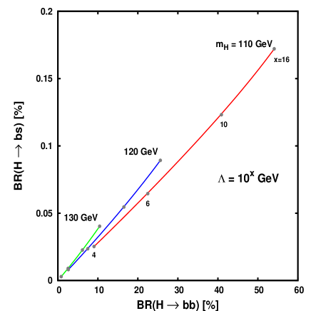
In Fig.7, we show correlations between BR and BR, for 110, 120, 130 GeV. For each value, we show by grey bubbles the points corresponding to GeV, that are univocally set by BR, for any given . Note that the dependence in the slopes is much reduced with respect to the flavor-diagonal decay correlations in Fig.5 (right). This is because, in the Eqs.(11)-(13) for the FC couplings, the dependence on is subdominant (i.e., depleted by radiative couplings) with respect to the Eqs.(4)-(7) for the flavor-diagonal couplings, where terms are enhanced by the ChSB fermion masses.
In Table 5, we report the expected number of events for the FC Higgs decay , corresponding to the production channel at GeV and with integrated luminosity of 500 fb-1. One can see that 18 (120) events are expected for and GeV, decreasing to 2.1 (10) for and GeV. Considering the moderate background environment of the linear collider, we then expect that a detailed study including backgrounds and detection efficiencies could confirm the possibility of making a measurement of BR for a quite wide range of the model parameters.
6 Conclusions
In this paper, we examined the potential of a linear collider program for testing the effective Yukawa scenario. With respect to the SM, this theoretical framework is characterized by a Higgs boson with radiative (and hence depleted) Yukawa couplings to fermions, and unaltered couplings to EW massive vector bosons. LHC will be able to pinpoint this scenario that, at hadron colliders, for GeV, foresees a Higgs boson mainly produced by vector-boson fusion with SM cross sections, with enhanced decays to . The direct investigation of the fermionic sector of the Higgs-boson couplings requires instead the clean environment of a linear collider program. We showed, that, with a typical setup with GeV and 500 fb-1 of integrated luminosity, the production rates for a Higgs boson decaying into are sufficiently large to allow a nice determination of the corresponding effective Yukawa couplings, for GeV. Furthermore, since fermionic BR’s are particularly sensitive to the large energy scale (where the Yukawa couplings are assumed to vanish at tree level), a measurement of the high-statistic channel is expected to provide a good determination even for GeV, where the sensitivity to the scale of BR decreases. Another sector where LHC can not compete with a linear collider is the study of the enhanced FC Higgs-boson decay , for which the low hadronic background of a linear collider is vital for detection. In particular, we showed that BR, that is almost of the same order of BR and BR, is expected for , with a corresponding event statistic sufficient for a nice BR determination. More detailed conclusions will require a more refined phenomenological analysis including the relevant backgrounds and detection efficiencies.
Acknowledgments
We would like to thank Gad Eilam for pointing out reference [12]. B.M. was partially supported by the RTN European Programme Contract No. MRTN-CT-2006-035505 (HEPTOOLS, Tools and Precision Calculations for Physics Discoveries at Colliders).
References
- [1] For a review see e.g. A. Djouadi, Phys. Rept. 457, 1 (2008), arXiv:hep-ph/0503172.
- [2] J. A. Aguilar-Saavedra et al. [ECFA/DESY LC Physics Working Group], “TESLA Technical Design Report Part III: Physics at an e+e- Linear Collider”, R.D.Heuer, D.Miller, F.Richard, P.Zerwas, Eds., arXiv:hep-ph/0106315, http://tesla.desy.de/newpages/TDRCD/start.html .
- [3] E. Accomando et al. [CLIC Physics Working Group], “Physics at the CLIC multi-TeV linear collider”, M. Battaglia, A. De Roeck, J. Ellis, D. Schulte, Eds., CERN-2004-005, arXiv:hep-ph/0412251.
- [4] E. Gabrielli and B. Mele, Phys. Rev. D 82, 113014 (2010), arXiv:1005.2498 [hep-ph].
- [5] See, for instance, H. E. Haber, G. L. Kane and T. Sterling, Nucl. Phys. B 161, 493 (1979); J. F. Gunion, R. Vega and J. Wudka, Phys. Rev. D 42, 1673 (1990); P. Bamert and Z. Kunszt, Phys. Lett. B 306, 335 (1993), arXiv:hep-ph/9303239; A. G. Akeroyd, Phys. Lett. B 368, 89 (1996), arXiv:hep-ph/9511347; A. Barroso, L. Brucher and R. Santos, Phys. Rev. D 60, 035005 (1999), arXiv:hep-ph/9901293; L. Brucher and R. Santos, Eur. Phys. J. C 12, 87 (2000), arXiv:hep-ph/9907434.
- [6] R. Barate et al. (LEP Working Group for Higgs Boson Searches and ALEPH Collaboration), Phys. Lett. B 565, 61 (2003), arXiv:hep-ex/0306033.
- [7] CDF and D0 collaborations, Phys. Rev. Lett. 104, 061802 (2010); updated in arXiv:1007.4587 [hep-ex].
- [8] G. Aarons et al. [ILC Collaboration], “International Linear Collider Reference Design Report, Volume 2: PHYSICS AT THE ILC”, A.Djouadi, J.Lykken, K.Mönig, Y.Okada, M.Oreglia, S.Yamashita, Eds., arXiv:0709.1893 [hep-ph].
- [9] M. Battaglia, “The International Linear Collider”, arXiv:0705.3997 [hep-ex].
- [10] M. Battaglia, “Measuring Higgs branching ratios and telling the SM from a MSSM Higgs boson at the e+ e- linear collider”, arXiv:hep-ph/9910271.
- [11] G. Eilam, B. Haeri and A. Soni, Phys. Rev. D 41, 875 (1990).
- [12] A. Arhrib, Phys. Lett. B 612, 263 (2005), arXiv:hep-ph/0409218.
- [13] A. M. Curiel, M. J. Herrero and D. Temes, Phys. Rev. D 67, 075008 (2003), arXiv:hep-ph/0210335; A. M. Curiel, M. J. Herrero, W. Hollik, F. Merz and S. Penaranda, Phys. Rev. D 69, 075009 (2004), arXiv:hep-ph/0312135; S. Bejar, J. Guasch and J. Sola, JHEP 0510, 113 (2005), arXiv:hep-ph/0508043; W. Hollik, S. Penaranda and M. Vogt, Eur. Phys. J. C 47, 207 (2006), arXiv:hep-ph/0511021; S. Bejar, F. Dilme, J. Guasch and J. Sola, JHEP 0408, 018 (2004), arXiv:hep-ph/0402188; A. Arhrib, D. K. Ghosh, O. C. W. Kong and R. D. Vaidya, Phys. Lett. B 647, 36 (2007), arXiv:hep-ph/0605056; S. Bejar, J. Guasch, D. Lopez-Val and J. Sola, Phys. Lett. B 668, 364 (2008), arXiv:0805.0973 [hep-ph].
- [14] H. Arason, D. J. Castano, B. Keszthelyi, S. Mikaelian, E. J. Piard, P. Ramond and B. D. Wright, Phys. Rev. D 46 (1992) 3945.
- [15] D. Atwood, L. Reina and A. Soni, Phys. Rev. D 55, 3156 (1997), arXiv:hep-ph/9609279.
- [16] K. Nakamura et al. [Particle Data Group], “Review of particle physics”, J. Phys. G 37, 075021 (2010).
- [17] J. Laiho, E. Lunghi and R. S. Van de Water, Phys. Rev. D 81, 034503 (2010), arXiv:0910.2928 [hep-ph].
- [18] E. Golowich, J. Hewett, S. Pakvasa, A. A. Petrov and G. K. Yeghiyan, arXiv:1102.0009 [hep-ph].