Fractional variational problems
depending on indefinite integrals

Abstract

We obtain necessary optimality conditions for variational problems with a Lagrangian depending on a Caputo fractional derivative, a fractional and an indefinite integral. Main results give fractional Euler–Lagrange type equations and natural boundary conditions, which provide a generalization of previous results found in the literature. Isoperimetric problems, problems with holonomic constraints and depending on higher-order Caputo derivatives, as well as fractional Lagrange problems, are considered.

MSC 2010: 49K05, 49S05, 26A33, 34A08.

Keywords: calculus of variations, fractional calculus, Caputo derivatives, fractional necessary optimality equations.

1 Introduction

In the 18th century, Euler considered the problem of optimizing functionals depending not only on some unknown function $y$ and some derivative of $y$, but also on an antiderivative of $y$ (see [19]). Similar problems have been recently investigated in [24], where Lagrangians containing higher-order derivatives and optimal control problems are considered. More generally, it has been shown that the results of [24] hold on an arbitrary time scale [30]. Here we study such problems within the framework of fractional calculus.

Roughly speaking, a fractional calculus defines integrals and derivatives of non-integer order. Let $\alpha>0$ be a real number and $n\in\mathbb{N}$ be such that $n-1<\alpha<n$. Here we follow [8] and [26, 31]. Let $f:[a,b]\to\mathbb{R}$ be piecewise continuous on $(a,b)$ and integrable on $[a,b]$. The left and right Riemann–Liouville fractional integrals of $f$ of order $\alpha$ are defined respectively by

$${{}_{a}I_{x}^{\alpha}}f(x)=\frac{1}{\Gamma(\alpha)}\int_{a}^{x}(x-t)^{\alpha-1}f(t)dt\quad\mbox{and}\quad{{}_{x}I_{b}^{\alpha}}f(x)=\frac{1}{\Gamma(\alpha)}\int_{x}^{b}(t-x)^{\alpha-1}f(t)dt.$$

Here $\Gamma$ is the well-known Gamma function. Then the left ${{}_{a}D_{x}^{\alpha}}$ and right ${{}_{x}D_{b}^{\alpha}}$ Riemann–Liouville fractional derivatives of $f$ of order $\alpha$ are defined (if they exist) as

$${{}_{a}D_{x}^{\alpha}}f(x)=\frac{1}{\Gamma(n-\alpha)}\frac{d^{n}}{dx^{n}}\int_{a}^{x}(x-t)^{n-\alpha-1}f(t)dt$$ (1)

and

$${{}_{x}D_{b}^{\alpha}}f(x)=\frac{(-1)^{n}}{\Gamma(n-\alpha)}\frac{d^{n}}{dx^{n}}\int_{x}^{b}(t-x)^{n-\alpha-1}f(t)dt.$$ (2)

The fractional derivatives (1) and (2) have one disadvantage when modeling real world phenomena: the fractional derivative of a constant is not zero. To eliminate this problem, one often considers fractional derivatives in the sense of Caputo. Let $f$ belong to the space $AC^{n}([a,b];\mathbb{R})$ of absolutely continuous functions. The left and right Caputo fractional derivatives of $f$ of order $\alpha$ are defined respectively by

$${{}_{a}^{C}D_{x}^{\alpha}}f(x)=\frac{1}{\Gamma(n-\alpha)}\int_{a}^{x}(x-t)^{n-\alpha-1}f^{(n)}(t)dt$$

and

$${{}_{x}^{C}D_{b}^{\alpha}}f(x)=\frac{1}{\Gamma(n-\alpha)}\int_{x}^{b}(-1)^{n}(t-x)^{n-\alpha-1}f^{(n)}(t)dt.$$

These fractional integrals and derivatives define a rich calculus. For details see the books [26, 31, 39]. Here we just recall a useful property for our purposes: integration by parts. For fractional integrals,

$$\int_{a}^{b}g(x)\cdot{{}_{a}I_{x}^{\alpha}}f(x)dx=\int_{a}^{b}f(x)\cdot{{}_{x}I_{b}^{\alpha}}g(x)dx$$

(see, e.g., [26, Lemma 2.7]), and for Caputo fractional derivatives

$$\int_{a}^{b}g(x)\cdot{{}_{a}^{C}D_{x}^{\alpha}}f(x)dx=\displaystyle\int_{a}^{b}f(x)\cdot{{}_{x}D_{b}^{\alpha}}g(x)dx+\sum_{j=0}^{n-1}\left[{{}_{x}D_{b}^{\alpha+j-n}}g(x)\cdot f^{(n-1-j)}(x)\right]_{a}^{b}$$

(see, e.g., [3, Eq. (16)]). In particular, for $\alpha\in(0,1)$ one has

$$\int_{a}^{b}g(x)\cdot{{}_{a}^{C}D_{x}^{\alpha}}f(x)dx=\int_{a}^{b}f(x)\cdot{{}_{x}D_{b}^{\alpha}}g(x)dx+\left[{{}_{x}I_{b}^{1-\alpha}}g(x)\cdot f(x)\right]_{a}^{b}.$$ (3)

When $\alpha\rightarrow 1$, ${{}_{a}^{C}D_{x}^{\alpha}}=\frac{d}{dx}$, ${{}_{x}D_{b}^{\alpha}}=-\frac{d}{dx}$, ${{}_{x}I_{b}^{1-\alpha}}$ is the identity operator, and (3) gives the classical formula of integration by parts.

The fractional calculus of variations concerns finding extremizers for variational functionals depending on fractional derivatives instead of integer ones. The theory started in 1996 with the work of Riewe, in order to better describe non-conservative systems in mechanics [37, 38]. The subject is now under strong development due to its many applications in physics and engineering, providing more accurate models of physical phenomena (see, e.g., [4, 9, 12, 14, 15, 18, 20, 21, 33, 35]). With respect to results on fractional variational calculus via Caputo operators, we refer the reader to [2, 5, 10, 23, 28, 32, 34] and references therein.

Our main contribution is an extension of the results presented in [2, 24] by considering Lagrangians containing an antiderivative, that in turn depend on the unknown function, a fractional integral, and a Caputo fractional derivative (Section 2). Transversality conditions are studied in Section 3, where the variational functional $J$ depends also on the terminal time $T$, $J(y,T)$, and where we obtain conditions for a pair $(y,T)$ to be an optimal solution to the problem. In Section 4 we consider isoperimetric problems with integral constraints of the same type as the cost functionals considered in Section 2. Fractional problems with holonomic constraints are considered in Section 5. The situation when the Lagrangian depends on higher order Caputo derivatives, i.e., it depends on ${}^{C}_{a}D_{x}^{\alpha_{k}}y(x)$ for $\alpha_{k}\in(k-1,k)$, $k\in\{1,\ldots,n\}$, is studied in Section 6, while Section 7 considers fractional Lagrange problems and the Hamiltonian approach. In Section 8 we obtain sufficient conditions of optimization under suitable convexity assumptions on the Lagrangian. We end with Section 9, discussing a numerical scheme for solving the proposed fractional variational problems. The idea is to approximate fractional problems by classical ones. Numerical results for two illustrative examples are described in detail.

2 The fundamental problem

Let $\alpha\in(0,1)$ and $\beta>0$. The problem that we address is stated in the following way. Minimize the cost functional

$$J(y)=\int_{a}^{b}L(x,y(x),{{}^{C}_{a}D_{x}^{\alpha}}y(x),{{}_{a}I_{x}^{\beta}}y(x),z(x))dx,$$ (4)

where the variable $z$ is defined by

$$z(x)=\int_{a}^{x}l(t,y(t),{{}^{C}_{a}D_{t}^{\alpha}}y(t),{{}_{a}I_{t}^{\beta}}y(t))dt,$$

subject to the boundary conditions

$$y(a)=y_{a}\quad\mbox{and}\quad y(b)=y_{b}.$$ (5)

We assume that the functions $(x,y,v,w,z)\to L(x,y,v,w,z)$ and $(x,y,v,w)\to l(x,y,v,w)$ are of class $C^{1}$, and the trajectories $y:[a,b]\to\mathbb{R}$ are absolute continuous functions, $y\in AC([a,b];\mathbb{R})$, such that ${{}^{C}_{a}D_{x}^{\alpha}}y(x)$ and ${{}_{a}I_{x}^{\beta}}y(x)$ exist and are continuous on $[a,b]$. We denote such class of functions by $\mathcal{F}([a,b];\mathbb{R})$. Also, to simplify, by $[\cdot]$ and $\{\cdot\}$ we denote the operators

$$[y](x)=(x,y(x),{{}^{C}_{a}D_{x}^{\alpha}}y(x),{{}_{a}I_{x}^{\beta}}y(x),z(x))\quad\mbox{and}\quad\{y\}(x)=(x,y(x),{{}^{C}_{a}D_{x}^{\alpha}}y(x),{{}_{a}I_{x}^{\beta}}y(x)).$$

Theorem 1.

Let $y\in\mathcal{F}([a,b];\mathbb{R})$ be a minimizer of $J$ as in (4), subject to the boundary conditions (5). Then, for all $x\in[a,b]$, $y$ is a solution of the fractional equation

$$\frac{\partial L}{\partial y}[y](x)+{{}_{x}D^{\alpha}_{b}}\left(\frac{\partial L}{\partial v}[y](x)\right)+{{}_{x}I_{b}^{\beta}}\left(\frac{\partial L}{\partial w}[y](x)\right)+\int_{x}^{b}\frac{\partial L}{\partial z}[y](t)dt\cdot\frac{\partial l}{\partial y}\{y\}(x)\\ +{{}_{x}D^{\alpha}_{b}}\left(\int_{x}^{b}\frac{\partial L}{\partial z}[y](t)dt\cdot\frac{\partial l}{\partial v}\{y\}(x)\right)+{{}_{x}I^{\beta}_{b}}\left(\int_{x}^{b}\frac{\partial L}{\partial z}[y](t)dt\cdot\frac{\partial l}{\partial w}\{y\}(x)\right)=0.$$ (6)

Proof.

Let $h\in\mathcal{F}([a,b];\mathbb{R})$ be such that $h(a)=0=h(b)$, and $\epsilon$ be a real number with $|\epsilon|\ll 1$. If we define $j$ as $j(\epsilon)=J(y+\epsilon h)$, then $j^{\prime}(0)=0$. Differentiating $j$ at $\epsilon=0$, we get

$$\int_{a}^{b}\left[\frac{\partial L}{\partial y}[y](x)h(x)+\frac{\partial L}{\partial v}[y](x){{}^{C}_{a}D^{\alpha}_{x}}h(x)+\frac{\partial L}{\partial w}[y](x){{}_{a}I^{\beta}_{x}}h(x)\right.\\ \left.+\frac{\partial L}{\partial z}[y](x)\int_{a}^{x}\left(\frac{\partial l}{\partial y}\{y\}(t)h(t)+\frac{\partial l}{\partial v}\{y\}(t){{}^{C}_{a}D^{\alpha}_{t}}h(t)+\frac{\partial l}{\partial w}\{y\}(t){{}_{a}I^{\beta}_{t}}h(t)\right)dt\right]dx=0.$$

The necessary condition (6) follows from the next relations and the fundamental lemma of the calculus of variations (cf., e.g., [41, p. 32]):

$$\int_{a}^{b}\frac{\partial L}{\partial v}[y](x){{}^{C}_{a}D^{\alpha}_{x}}h(x)dx=\int_{a}^{b}{{}_{x}D_{b}^{\alpha}}\left(\frac{\partial L}{\partial v}[y](x)\right)h(x)dx+\left[{{}_{x}I_{b}^{1-\alpha}}\left(\frac{\partial L}{\partial v}[y](x)\right)h(x)\right]_{a}^{b},$$

$$\int_{a}^{b}\frac{\partial L}{\partial w}[y](x){{}_{a}I^{\beta}_{x}}h(x)dx=\int_{a}^{b}{{}_{x}I_{b}^{\beta}}\left(\frac{\partial L}{\partial w}[y](x)\right)h(x)dx,$$

$$\int_{a}^{b} \frac{\partial L}{\partial z}[y](x)\left(\int_{a}^{x}\frac{\partial l}{\partial y}\{y\}(t)h(t)dt\right)dx=\int_{a}^{b}\left(-\frac{d}{dx}\int_{x}^{b}\frac{\partial L}{\partial z}[y](t)dt\right)\left(\int_{a}^{x}\frac{\partial l}{\partial y}\{y\}(t)h(t)dt\right)dx$$

$$=\left[-\left(\int_{x}^{b}\frac{\partial L}{\partial z}[y](t)dt\right)\left(\int_{a}^{x}\frac{\partial l}{\partial y}\{y\}(t)h(t)dt\right)\right]_{a}^{b}+\int_{a}^{b}\left(\int_{x}^{b}\frac{\partial L}{\partial z}[y](t)dt\right)\frac{\partial l}{\partial y}\{y\}(x)h(x)\,dx$$

$$=\int_{a}^{b}\left(\int_{x}^{b}\frac{\partial L}{\partial z}[y](t)dt\right)\frac{\partial l}{\partial y}\{y\}(x)h(x)\,dx,$$

$$\int_{a}^{b} \frac{\partial L}{\partial z}[y](x)\left(\int_{a}^{x}\frac{\partial l}{\partial v}\{y\}(t){{}^{C}_{a}D^{\alpha}_{t}}h(t)dt\right)dx=\int_{a}^{b}\left(-\frac{d}{dx}\int_{x}^{b}\frac{\partial L}{\partial z}[y](t)dt\right)\left(\int_{a}^{x}\frac{\partial l}{\partial v}\{y\}(t){{}^{C}_{a}D^{\alpha}_{t}}h(t)dt\right)dx$$

$$=\left[-\left(\int_{x}^{b}\frac{\partial L}{\partial z}[y](t)dt\right)\left(\int_{a}^{x}\frac{\partial l}{\partial v}\{y\}(t){{}^{C}_{a}D^{\alpha}_{t}}h(t)dt\right)\right]_{a}^{b}+\int_{a}^{b}\left(\int_{x}^{b}\frac{\partial L}{\partial z}[y](t)dt\right)\frac{\partial l}{\partial v}\{y\}(x){{}^{C}_{a}D^{\alpha}_{x}}h(x)\,dx$$

$$=\int_{a}^{b}{{}_{x}D^{\alpha}_{b}}\left(\int_{x}^{b}\frac{\partial L}{\partial z}[y](t)dt\frac{\partial l}{\partial v}\{y\}(x)\right)h(x)\,dx+\left[{{}_{x}I^{1-\alpha}_{b}}\left(\int_{x}^{b}\frac{\partial L}{\partial z}[y](t)dt\frac{\partial l}{\partial v}\{y\}(x)\right)h(x)\right]_{a}^{b},$$

and

$$\int_{a}^{b}\frac{\partial L}{\partial z}[y](x)\left(\int_{a}^{x}\frac{\partial l}{\partial w}\{y\}(t){{}_{a}I^{\beta}_{t}}h(t)dt\right)dx=\int_{a}^{b}{{}_{x}I^{\beta}_{b}}\left(\int_{x}^{b}\frac{\partial L}{\partial z}[y](t)dt\frac{\partial l}{\partial w}\{y\}(x)\right)h(x)\,dx.$$

∎

The fractional Euler–Lagrange equation (6) involves not only fractional integrals and fractional derivatives, but also indefinite integrals. Theorem 1 gives a necessary condition to determine the possible choices for extremizers.

Definition 2.

Solutions to the fractional Euler–Lagrange equation (6) are called extremals for $J$ defined by (4).

Example 3.

Consider the functional

$$J(y)=\int_{0}^{1}\left[({{}^{C}_{0}D_{x}^{\alpha}}y(x)-\Gamma(\alpha+2)x)^{2}+z(x)\right]dx,$$ (7)

where $\alpha\in(0,1)$ and

$$z(x)=\int_{0}^{x}(y(t)-t^{\alpha+1})^{2}\,dt,$$

defined on the set

$$\left\{y\in\mathcal{F}([0,1];\mathbb{R}):\,y(0)=0\,\mbox{ and }\,y(1)=1\right\}.$$

Let

$$y_{\alpha}(x)=x^{\alpha+1},\quad x\in[0,1].$$ (8)

Then,

$${{}^{C}_{0}D_{x}^{\alpha}}y_{\alpha}(x)=\Gamma(\alpha+2)x.$$

Since $J(y)\geq 0$ for all admissible functions $y$, and $J(y_{\alpha})=0$, we have that $y_{\alpha}$ is a minimizer of $J$. The Euler–Lagrange equation applied to (7) gives

$${{}_{x}D_{1}^{\alpha}}({{}^{C}_{0}D_{x}^{\alpha}}y(x)-\Gamma(\alpha+2)x)+\int_{x}^{1}1dt\,(y(x)-x^{\alpha+1})=0.$$ (9)

Obviously, $y_{\alpha}$ is a solution of the fractional differential equation (9).

The extremizer (8) of Example 3 is smooth on the closed interval $[0,1]$. This is not always the case. As next example shows, minimizers of (4)–(5) are not necessarily $C^{1}$ functions.

Example 4.

Consider the following fractional variational problem: to minimize the functional

$$J(y)=\int_{0}^{1}\left[\left({{}^{C}_{0}D_{x}^{\alpha}}y(x)-1\right)^{2}+z(x)\right]dx$$ (10)

on

$$\left\{y\in\mathcal{F}([0,1];\mathbb{R})\,:\,y(0)=0\quad\mbox{and}\quad y(1)=\frac{1}{\Gamma(\alpha+1)}\right\},$$

where $z$ is given by

$$z(x)=\int_{0}^{x}\left(y(t)-\frac{t^{\alpha}}{\Gamma(\alpha+1)}\right)^{2}dt.$$

Since ${{}^{C}_{0}D_{x}^{\alpha}}x^{\alpha}=\Gamma(\alpha+1)$, we deduce easily that function

$$\overline{y}(x)=\frac{x^{\alpha}}{\Gamma(\alpha+1)}$$ (11)

is the global minimizer to the problem. Indeed, $J(y)\geq 0$ for all $y$, and $J(\overline{y})=0$. Let us see that $\overline{y}$ is an extremal for $J$. The fractional Euler–Lagrange equation (6) becomes

$$2\,{{}_{x}D_{1}^{\alpha}}({{}^{C}_{0}D_{x}^{\alpha}}y(x)-1)+\int_{x}^{1}1\,dt\cdot 2\left(y(x)-\frac{x^{\alpha}}{\Gamma(\alpha+1)}\right)=0.$$ (12)

Obviously, $\overline{y}$ is a solution of equation (12).

Remark 5.

The minimizer (11) of Example 4 is not differentiable at 0, as $0<\alpha<1$. However, $\overline{y}(0)=0$ and ${{}^{C}_{0}D_{x}^{\alpha}}\overline{y}(x)={{}_{0}D_{x}^{\alpha}}\overline{y}(x)=\Gamma(\alpha+1)$ for any $x\in[0,1]$.

Corollary 6 (cf. equation (9) of [2]).

If $y$ is a minimizer of

$$J(y)=\int_{a}^{b}L(x,y(x),{{}^{C}_{a}D_{x}^{\alpha}}y(x))dx,$$ (13)

subject to the boundary conditions (5), then $y$ is a solution of the fractional equation

$$\frac{\partial L}{\partial y}[y](x)+{{}_{x}D^{\alpha}_{b}}\left(\frac{\partial L}{\partial v}[y](x)\right)=0.$$

Proof.

Follows from Theorem 1 with an $L$ that does not depend on ${{}_{a}I_{x}^{\beta}}y$ and $z$. ∎

We now derive the Euler–Lagrange equations for functionals containing several dependent variables, i.e., for functionals of type

$$J(y_{1},\ldots,y_{n})=\int_{a}^{b}L(x,y_{1}(x),\ldots,y_{n}(x),{{}^{C}_{a}D_{x}^{\alpha}}y_{1}(x),\ldots,{{}^{C}_{a}D_{x}^{\alpha}}y_{n}(x),{{}_{a}I_{x}^{\beta}}y_{1}(x),\ldots,{{}_{a}I_{x}^{\beta}}y_{n}(x),z(x))dx,$$ (14)

where $n\in\mathbb{N}$ and $z$ is defined by

$$z(x)=\int_{a}^{x}l(t,y_{1}(t),\ldots,y_{n}(t),{{}^{C}_{a}D_{t}^{\alpha}}y_{1}(t),\ldots,{{}^{C}_{a}D_{t}^{\alpha}}y_{n}(t),{{}_{a}I_{t}^{\beta}}y_{1}(t),\ldots,{{}_{a}I_{t}^{\beta}}y_{n}(t))dt,$$

subject to the boundary conditions

$$y_{k}(a)=y_{a,k}\quad\mbox{and}\quad y_{k}(b)=y_{b,k},\quad k\in\{1,\ldots,n\}.$$ (15)

To simplify, we consider $y$ as the vector $y=(y_{1},\ldots,y_{n})$. Consider a family of variations $y+\epsilon h$, where $|\epsilon|\ll 1$ and $h=(h_{1},\ldots,h_{n})$. The boundary conditions (15) imply that $h_{k}(a)=0=h_{k}(b)$, for $k\in\{1,\ldots,n\}$. The following theorem can be easily proved.

Theorem 7.

Let $y$ be a minimizer of $J$ as in (14), subject to the boundary conditions (15). Then, for all $k\in\{1,\ldots,n\}$ and for all $x\in[a,b]$, $y$ is a solution of the fractional Euler–Lagrange equation

$$\frac{\partial L}{\partial y_{k}}[y](x)+{{}_{x}D^{\alpha}_{b}}\left(\frac{\partial L}{\partial v_{k}}[y](x)\right)+{{}_{x}I^{\beta}_{b}}\left(\frac{\partial L}{\partial w_{k}}[y](x)\right)+\int_{x}^{b}\frac{\partial L}{\partial z}[y](t)dt\cdot\frac{\partial l}{\partial y_{k}}\{y\}(x)\\ +{{}_{x}D^{\alpha}_{b}}\left(\int_{x}^{b}\frac{\partial L}{\partial z}[y](t)dt\cdot\frac{\partial l}{\partial v_{k}}\{y\}(x)\right)+{{}_{x}I^{\beta}_{b}}\left(\int_{x}^{b}\frac{\partial L}{\partial z}[y](t)dt\cdot\frac{\partial l}{\partial w_{k}}\{y\}(x)\right)=0.$$

3 Natural boundary conditions

In this section we consider a more general question. Not only the unknown function $y$ is a variable in the problem, but also the terminal time $T$ is an unknown. For $T\in[a,b]$, consider the functional

$$J(y,T)=\int_{a}^{T}L[y](x)dx,$$ (16)

where

$$[y](x)=(x,y(x),{{}^{C}_{a}D_{x}^{\alpha}}y(x),{{}_{a}I_{x}^{\beta}}y(x),z(x)).$$

The problem consists in finding a pair $(y,T)\in\mathcal{F}([a,b];\mathbb{R})\times[a,b]$ for which the functional $J$ attains a minimum value. First we give a remark that will be used later in the proof of Theorem 9.

Remark 8.

If $\phi$ is a continuous function, then (cf. [31, p. 46])

$$\lim_{x\to T}{{}_{x}I_{T}^{1-\alpha}}\phi(x)=0$$

for any $\alpha\in(0,1)$.

Theorem 9.

Let $(y,T)$ be a minimizer of $J$ as in (16). Then, for all $x\in[a,T]$, $(y,T)$ is a solution of the fractional equation

$$\frac{\partial L}{\partial y}[y](x)+{{}_{x}D^{\alpha}_{T}}\left(\frac{\partial L}{\partial v}[y](x)\right)+{{}_{x}I_{T}^{\beta}}\left(\frac{\partial L}{\partial w}[y](x)\right)+\int_{x}^{T}\frac{\partial L}{\partial z}[y](t)dt\cdot\frac{\partial l}{\partial y}\{y\}(x)\\ +{{}_{x}D^{\alpha}_{T}}\left(\int_{x}^{T}\frac{\partial L}{\partial z}[y](t)dt\cdot\frac{\partial l}{\partial v}\{y\}(x)\right)+{{}_{x}I^{\beta}_{T}}\left(\int_{x}^{T}\frac{\partial L}{\partial z}[y](t)dt\cdot\frac{\partial l}{\partial w}\{y\}(x)\right)=0$$

and satisfies the transversality conditions

$$\left[{{}_{x}I_{T}^{1-\alpha}}\left(\frac{\partial L}{\partial v}[y](x)+\int_{x}^{T}\frac{\partial L}{\partial z}[y](t)\,dt\cdot\frac{\partial l}{\partial v}\{y\}(x)\right)\right]_{x=a}=0$$

and

$$L[y](T)=0.$$

Proof.

Let $h\in\mathcal{F}([a,b];\mathbb{R})$ be a variation, and let $\triangle T$ be a real number. Define the function

$$j(\epsilon)=J(y+\epsilon h,T+\epsilon\triangle T)$$

with $|\epsilon|\ll 1$. Differentiating $j$ at $\epsilon=0$, and using the same procedure as in Theorem 1, we deduce that

$$\triangle T\cdot L[y](T)+\int_{a}^{T}\left[\frac{\partial L}{\partial y}[y](x)+{{}_{x}D^{\alpha}_{T}}\left(\frac{\partial L}{\partial v}[y](x)\right)+{{}_{x}I_{T}^{\beta}}\left(\frac{\partial L}{\partial w}[y](x)\right)+\int_{x}^{T}\frac{\partial L}{\partial z}[y](t)dt\cdot\frac{\partial l}{\partial y}\{y\}(x)\right.\\ \left.+{{}_{x}D^{\alpha}_{T}}\left(\int_{x}^{T}\frac{\partial L}{\partial z}[y](t)dt\cdot\frac{\partial l}{\partial v}\{y\}(x)\right)+{{}_{x}I^{\beta}_{T}}\left(\int_{x}^{T}\frac{\partial L}{\partial z}[y](t)dt\cdot\frac{\partial l}{\partial w}\{y\}(x)\right)\right]h(x)dx\\ +\left[{{}_{x}I_{T}^{1-\alpha}}\left(\frac{\partial L}{\partial v}[y](x)\right)h(x)\right]_{a}^{T}+\left[{{}_{x}I^{1-\alpha}_{T}}\left(\int_{x}^{T}\frac{\partial L}{\partial z}[y](t)dt\cdot\frac{\partial l}{\partial v}\{y\}(x)\right)h(x)\right]_{a}^{T}=0.$$

The theorem follows from the arbitrariness of $h$ and $\triangle T$. ∎

Remark 10.

If $T$ is fixed, say $T=b$, then $\triangle T=0$ and the transversality conditions reduce to

$$\left[{{}_{x}I_{b}^{1-\alpha}}\left(\frac{\partial L}{\partial v}[y](x)+\int_{x}^{b}\frac{\partial L}{\partial z}[y](t)\,dt\cdot\frac{\partial l}{\partial v}\{y\}(x)\right)\right]_{a}=0.$$ (17)

Example 11.

Consider the problem of minimizing the functional $J$ as in (10), but without given boundary conditions. Besides equation (12), extremals must also satisfy

$$\left[{{}_{x}I_{1}^{1-\alpha}}\left({{}^{C}_{0}D_{x}^{\alpha}}y(x)-1\right)\right]_{0}=0.$$ (18)

Again, $\overline{y}$ given by (11) is a solution of (12) and (18).

As a particular case, the following result of [2] is deduced.

Corollary 12 (cf. equations (9) and (12) of [2]).

If $y$ is a minimizer of $J$ as in (13), then $y$ is a solution of

$$\frac{\partial L}{\partial y}[y](x)+{{}_{x}D^{\alpha}_{b}}\left(\frac{\partial L}{\partial v}[y](x)\right)=0$$

and satisfies the transversality condition

$$\left[{{}_{x}I_{b}^{1-\alpha}}\left(\frac{\partial L}{\partial v}[y](x)\right)\right]_{a}=0.$$

Proof.

The Lagrangian $L$ in (13) does not depend on ${{}_{a}I_{x}^{\beta}}y$ and $z$, and the result follows from Theorem 9. ∎

Remark 13.

Observe that the condition

$$\left[{{}_{x}I_{b}^{1-\alpha}}\left(\frac{\partial L}{\partial v}[y](x)\right)\right]_{b}=0$$

is implicitly satisfied in Corollary 12 (cf. Remark 8).

4 Fractional isoperimetric problems

An isoperimetric problem deals with the question of optimizing a given functional under the presence of an integral constraint. This is a very old question, with its origins in the ancient Greece. They where interested in determining the shape of a closed curve with a fixed length and maximum area. This problem is known as Dido’s problem, and is an example of an isoperimetric problem of the calculus of variations [41]. For recent advancements on the subject we refer the reader to [6, 7, 17, 27] and references therein. In our case, within the fractional context, we state the isoperimetric problem in the following way. Determine the minimizers of a given functional

$$J(y)=\int_{a}^{b}L(x,y(x),{{}^{C}_{a}D_{x}^{\alpha}}y(x),{{}_{a}I_{x}^{\beta}}y(x),z(x))dx$$ (19)

subject to the boundary conditions

$$y(a)=y_{a}\quad\mbox{and}\quad y(b)=y_{b}$$ (20)

and the fractional integral constraint

$$I(y)=\int_{a}^{b}G(x,y(x),{{}^{C}_{a}D_{x}^{\alpha}}y(x),{{}_{a}I_{x}^{\beta}}y(x),z(x))dx=\gamma,\quad\gamma\in\mathbb{R},$$ (21)

where $z$ is defined by

$$z(x)=\int_{a}^{x}l(t,y(t),{{}^{C}_{a}D_{t}^{\alpha}}y(t),{{}_{a}I_{t}^{\beta}}y(t))dt.$$

As usual, we assume that all the functions $(x,y,v,w,z)\to L(x,y,v,w,z)$, $(x,y,v,w)\to l(x,y,v,w)$, and $(x,y,v,w,z)\to G(x,y,v,w,z)$ are of class $C^{1}$.

Theorem 14.

Let $y$ be a minimizer of $J$ as in (19), under the boundary conditions (20) and isoperimetric constraint (21). Suppose that $y$ is not an extremal for $I$ in (21). Then there exists a constant $\lambda$ such that $y$ is a solution of the fractional equation

$$\frac{\partial F}{\partial y}[y](x)+{{}_{x}D^{\alpha}_{b}}\left(\frac{\partial F}{\partial v}[y](x)\right)+{{}_{x}I^{\beta}_{b}}\left(\frac{\partial F}{\partial w}[y](x)\right)+\int_{x}^{b}\frac{\partial F}{\partial z}[y](t)dt\cdot\frac{\partial l}{\partial y}\{y\}(x)\\ +{{}_{x}D^{\alpha}_{b}}\left(\int_{x}^{b}\frac{\partial F}{\partial z}[y](t)dt\cdot\frac{\partial l}{\partial v}\{y\}(x)\right)+{{}_{x}I^{\beta}_{b}}\left(\int_{x}^{b}\frac{\partial F}{\partial z}[y](t)dt\cdot\frac{\partial l}{\partial w}\{y\}(x)\right)=0,$$

where $F=L-\lambda G$, for all $x\in[a,b]$.

Proof.

Let $\epsilon_{1},\epsilon_{2}\in\mathbb{R}$ be two real numbers such that $|\epsilon_{1}|\ll 1$ and $|\epsilon_{2}|\ll 1$, with $\epsilon_{1}$ free and $\epsilon_{2}$ to be determined later, and let $h_{1}$ and $h_{2}$ be two functions satisfying

$$h_{1}(a)=h_{1}(b)=h_{2}(a)=h_{2}(b)=0.$$

Define functions $j$ and $i$ by

$$j(\epsilon_{1},\epsilon_{2})=J(y+\epsilon_{1}h_{1}+\epsilon_{2}h_{2})$$

and

$$i(\epsilon_{1},\epsilon_{2})=I(y+\epsilon_{1}h_{1}+\epsilon_{2}h_{2})-\gamma.$$

Doing analogous calculations as in the proof of Theorem 1, one has

$$\left.\frac{\partial i}{\partial\epsilon_{2}}\right|_{(0,0)}=\int_{a}^{b}\left[\frac{\partial G}{\partial y}[y](x)+{{}_{x}D^{\alpha}_{b}}\left(\frac{\partial G}{\partial v}[y](x)\right)+{{}_{x}I^{\alpha}_{b}}\left(\frac{\partial G}{\partial w}[y](x)\right)+\int_{x}^{b}\frac{\partial G}{\partial z}[y](t)dt\cdot\frac{\partial l}{\partial y}\{y\}(x)\right.\\ \left.+{{}_{x}D^{\alpha}_{b}}\left(\int_{x}^{b}\frac{\partial G}{\partial z}[y](t)dt\cdot\frac{\partial l}{\partial v}\{y\}(x)\right)+{{}_{x}I^{\beta}_{b}}\left(\int_{x}^{b}\frac{\partial G}{\partial z}[y](t)dt\cdot\frac{\partial l}{\partial w}\{y\}(x)\right)\right]h_{2}(x)\,dx.$$

By hypothesis, $y$ is not an extremal for $I$ and therefore there must exist a function $h_{2}$ for which

$$\left.\frac{\partial i}{\partial\epsilon_{2}}\right|_{(0,0)}\not=0.$$

Since $i(0,0)=0$, by the implicit function theorem there exists a function $\epsilon_{2}(\cdot)$, defined in some neighborhood of zero, such that

$$i(\epsilon_{1},\epsilon_{2}(\epsilon_{1}))=0.$$ (22)

On the other hand, $j$ attains a minimum value at $(0,0)$ when subject to the constraint (22). Because $\nabla i(0,0)\neq(0,0)$, by the Lagrange multiplier rule [41, p. 77] there exists a constant $\lambda$ such that

$$\nabla(j(0,0)-\lambda i(0,0))=(0,0).$$

So

$$\left.\frac{\partial j}{\partial\epsilon_{1}}\right|_{(0,0)}-\lambda\left.\frac{\partial i}{\partial\epsilon_{1}}\right|_{(0,0)}=0.$$

Differentiating $j$ and $i$ at zero, and doing the same calculations as before, we get the desired result. ∎

Using the abnormal Lagrange multiplier rule [41, p. 82], the previous result can be generalized to include the case when the minimizer is an extremal of $I$.

Theorem 15.

Let $y$ be a minimizer of $J$ as in (19), subject to the constraints (20) and (21). Then there exist two constants $\lambda_{0}$ and $\lambda$, not both zero, such that $y$ is a solution of equation

$$\frac{\partial K}{\partial y}[y](x)+{{}_{x}D^{\alpha}_{b}}\left(\frac{\partial K}{\partial v}[y](x)\right)+{{}_{x}I^{\beta}_{b}}\left(\frac{\partial K}{\partial w}[y](x)\right)+\int_{x}^{b}\frac{\partial K}{\partial z}[y](t)dt\cdot\frac{\partial l}{\partial y}\{y\}(x)\\ +{{}_{x}D^{\alpha}_{b}}\left(\int_{x}^{b}\frac{\partial K}{\partial z}[y](t)dt\cdot\frac{\partial l}{\partial v}\{y\}(x)\right)+{{}_{x}I^{\beta}_{b}}\left(\int_{x}^{b}\frac{\partial K}{\partial z}[y](t)dt\cdot\frac{\partial l}{\partial w}\{y\}(x)\right)=0$$

for all $x\in[a,b]$, where $K=\lambda_{0}L-\lambda G$.

Corollary 16 (cf. Theorem 3.4 of [10]).

Let $y$ be a minimizer of

$$J(y)=\int_{a}^{b}L(x,y(x),{{}^{C}_{a}D_{x}^{\alpha}}y(x))dx$$

subject to the boundary conditions

$$y(a)=y_{a}\quad\mbox{and}\quad y(b)=y_{b}$$

and the isoperimetric constraint

$$I(y)=\int_{a}^{b}G(x,y(x),{{}^{C}_{a}D_{x}^{\alpha}}y(x))dx=\gamma,\quad\gamma\in\mathbb{R}.$$

Then, there exist two constants $\lambda_{0}$ and $\lambda$, not both zero, such that $y$ is a solution of equation

$$\frac{\partial K}{\partial y}\left(x,y(x),{{}^{C}_{a}D_{x}^{\alpha}}y(x)\right)+{{}_{x}D^{\alpha}_{b}}\left(\frac{\partial K}{\partial v}\left(x,y(x),{{}^{C}_{a}D_{x}^{\alpha}}y(x)\right)\right)=0$$

for all $x\in[a,b]$, where $K=\lambda_{0}L-\lambda G$. Moreover, if $y$ is not an extremal for $I$, then we may take $\lambda_{0}=1$.

5 Holonomic constraints

In this section we consider the following problem. Minimize the functional

$$J(y_{1},y_{2})=\int_{a}^{b}L(x,y_{1}(x),y_{2}(x),{{}^{C}_{a}D_{x}^{\alpha}}y_{1}(x),{{}^{C}_{a}D_{x}^{\alpha}}y_{2}(x),{{}_{a}I_{x}^{\beta}}y_{1}(x),{{}_{a}I_{x}^{\beta}}y_{2}(x),z(x))dx,$$ (23)

where $z$ is defined by

$$z(x)=\int_{a}^{x}l(t,y_{1}(t),y_{2}(t),{{}^{C}_{a}D_{t}^{\alpha}}y_{1}(t),{{}^{C}_{a}D_{t}^{\alpha}}y_{2}(t),{{}_{a}I_{t}^{\beta}}y_{1}(t),{{}_{a}I_{t}^{\beta}}y_{2}(t))dt,$$

when restricted to the boundary conditions

$$(y_{1}(a),y_{2}(a))=(y_{1}^{a},y_{2}^{a})\mbox{ and }(y_{1}(b),y_{2}(b))=(y_{1}^{b},y_{2}^{b}),\quad y_{1}^{a},y_{2}^{a},y_{1}^{b},y_{2}^{b}\in\mathbb{R},$$ (24)

and the holonomic constraint

$$g(x,y_{1}(x),y_{2}(x))=0.$$ (25)

As usual, here

$$(x,y_{1},y_{2},v_{1},v_{2},w_{1},w_{2},z)\to L(x,y_{1},y_{2},v_{1},v_{2},w_{1},w_{2},z),$$

$$(x,y_{1},y_{2},v_{1},v_{2},w_{1},w_{2})\to l(x,y_{1},y_{2},v_{1},v_{2},w_{1},w_{2})$$

and

$$(x,y_{1},y_{2})\to g(x,y_{1},y_{2})$$

are all smooth. In what follows we make use of the operator $[\cdot,\cdot]$ given by

$$[y_{1},y_{2}](x)=(x,y_{1}(x),y_{2}(x),{{}^{C}_{a}D_{x}^{\alpha}}y_{1}(x),{{}^{C}_{a}D_{x}^{\alpha}}y_{2}(x),{{}_{a}I_{x}^{\beta}}y_{1}(x),{{}_{a}I_{x}^{\beta}}y_{2}(x),z(x))\,,$$

we denote $(x,y_{1}(x),y_{2}(x))$ by $(x,\mathbf{y}(x))$, and the Euler–Lagrange equation obtained in (6) with respect to $y_{i}$ by $(ELE_{i})$, $i=1,2$.

Remark 17.

For simplicity, we are considering functionals depending only on two functions $y_{1}$ and $y_{2}$. Theorem 18 is, however, easily generalized for $n$ variables $y_{1},\ldots,y_{n}$.

Theorem 18.

Let the pair $(y_{1},y_{2})$ be a minimizer of $J$ as in (23), subject to the constraints (24)–(25). If $\frac{\partial g}{\partial y_{2}}\not=0$, then there exists a continuous function $\lambda:[a,b]\to\mathbb{R}$ such that $(y_{1},y_{2})$ is a solution of

$$\frac{\partial F}{\partial y_{i}}[y_{1},y_{2}](x)+{{}_{x}D^{\alpha}_{b}}\left(\frac{\partial F}{\partial v_{i}}[y_{1},y_{2}](x)\right)+{{}_{x}I_{b}^{\beta}}\left(\frac{\partial F}{\partial w_{i}}[y_{1},y_{2}](x)\right)+\int_{x}^{b}\frac{\partial F}{\partial z}[y_{1},y_{2}](t)dt\cdot\frac{\partial l}{\partial y_{i}}\{y_{1},y_{2}\}(x)\\ +{{}_{x}D^{\alpha}_{b}}\left(\int_{x}^{b}\frac{\partial F}{\partial z}[y_{1},y_{2}](t)dt\cdot\frac{\partial l}{\partial v_{i}}\{y_{1},y_{2}\}(x)\right)+{{}_{x}I^{\beta}_{b}}\left(\int_{x}^{b}\frac{\partial F}{\partial z}[y_{1},y_{2}](t)dt\cdot\frac{\partial l}{\partial w_{i}}\{y_{1},y_{2}\}(x)\right)=0$$ (26)

for all $x\in[a,b]$ and $i=1,2$, where $F[y_{1},y_{2}](x)=L[y_{1},y_{2}](x)-\lambda(x)g(x,\mathbf{y}(x))$.

Proof.

Consider a variation of the optimal solution of type

$$(\overline{y}_{1},\overline{y}_{2})=(y_{1}+\epsilon h_{1},y_{2}+\epsilon h_{2}),$$

where $h_{1},h_{2}$ are two functions defined on $[a,b]$ satisfying

$$h_{1}(a)=h_{1}(b)=h_{2}(a)=h_{2}(b)=0,$$

and $\epsilon$ is a sufficiently small real parameter. Since $\frac{\partial g}{\partial y_{2}}(x,\overline{y}_{1}(x),\overline{y}_{2}(x))\not=0$ for all $x\in[a,b]$, we can solve equation $g(x,\overline{y}_{1}(x),\overline{y}_{2}(x))=0$ with respect to $h_{2}$, $h_{2}=h_{2}(\epsilon,h_{1})$. Differentiating $J(\overline{y}_{1},\overline{y}_{2})$ at $\epsilon=0$, and proceeding similarly as done in the proof of Theorem 1, we deduce that

$$\int_{a}^{b}(ELE_{1})h_{1}(x)+(ELE_{2})h_{2}(x)\,dx=0.$$ (27)

Besides, since $g(x,\overline{y}_{1}(x),\overline{y}_{2}(x))=0$, differentiating at $\epsilon=0$ we get

$$h_{2}(x)=-\frac{\frac{\partial g}{\partial y_{1}}(x,\mathbf{y}(x))}{\frac{\partial g}{\partial y_{2}}(x,\mathbf{y}(x))}h_{1}(x).$$ (28)

Define the function $\lambda$ on $[a,b]$ as

$$\lambda(x)=\frac{(ELE_{2})}{\frac{\partial g}{\partial y_{2}}(x,\mathbf{y}(x))}.$$ (29)

Combining (28) and (29), equation (27) can be written as

$$\int_{a}^{b}\left[(ELE_{1})-\lambda(x)\frac{\partial g}{\partial y_{1}}(x,\mathbf{y}(x))\right]h_{1}(x)\,dx=0.$$

By the arbitrariness of $h_{1}$, if follows that

$$(ELE_{1})-\lambda(x)\frac{\partial g}{\partial y_{1}}(x,\mathbf{y}(x))=0.$$

Define $F$ as

$$F[y_{1},y_{2}](x)=L[y_{1},y_{2}](x)-\lambda(x)g(x,\mathbf{y}(x)).$$

Then, equations (26) follow. ∎

6 Higher order Caputo derivatives

In this section we consider fractional variational problems, when in presence of higher order Caputo derivatives. We will restricted ourselves to the case where the orders are non integer, since the integer case is already well studied in the literature (for a modern account see [13, 16, 29]).

Let $n\in\mathbb{N}$, $\beta>0$, and $\alpha_{k}\in\mathbb{R}$ be such that $\alpha_{k}\in(k-1,k)$ for $k\in\{1,\ldots,n\}$. Admissible functions $y$ belong to $AC^{n}([a,b];\mathbb{R})$ and are such that ${{}^{C}_{a}D_{x}^{\alpha_{k}}}y$, $k=1,\ldots,n$, and ${{}_{a}I_{x}^{\beta}}y$ exist and are continuous on $[a,b]$. We denote such class of functions by $\mathcal{F}^{n}([a,b];\mathbb{R})$. For $\alpha=(\alpha_{1},\ldots,\alpha_{n})$, define the vector

$${{}_{a}^{C}D_{x}^{\alpha}}y(x)=({{}_{a}^{C}D_{x}^{\alpha_{1}}}y(x),\ldots,{{}_{a}^{C}D_{x}^{\alpha_{n}}}y(x)).$$ (30)

The optimization problem is the following: to minimize or maximize the functional

$$J(y)=\int_{a}^{b}L(x,y(x),{{}^{C}_{a}D_{x}^{\alpha}}y(x),{{}_{a}I_{x}^{\beta}}y(x),z(x))dx,$$ (31)

$y\in\mathcal{F}^{n}([a,b];\mathbb{R})$, subject to the boundary conditions

$$y^{(k)}(a)=y_{a,k}\quad\mbox{and}\quad y^{(k)}(b)=y_{b,k},\quad k\in\{0,\ldots,n-1\},$$ (32)

where $z:[a,b]\to\mathbb{R}$ is defined by

$$z(x)=\int_{a}^{x}l(t,y(t),{{}^{C}_{a}D_{t}^{\alpha}}y(t),{{}_{a}I_{t}^{\beta}}y(t))dt.$$

Theorem 19.

If $y\in\mathcal{F}^{n}([a,b];\mathbb{R})$ is a minimizer of $J$ as in (31), subject to the boundary conditions (32), then $y$ is a solution of the fractional equation

$$\frac{\partial L}{\partial y}[y](x)+\sum_{k=1}^{n}{{}_{x}D^{\alpha_{k}}_{b}}\left(\frac{\partial L}{\partial v_{k}}[y](x)\right)+{{}_{x}I^{\beta}_{b}}\left(\frac{\partial L}{\partial w}[y](x)\right)+\int_{x}^{b}\frac{\partial L}{\partial z}[y](t)dt\cdot\frac{\partial l}{\partial y}\{y\}(x)\\ +\sum_{k=1}^{n}{{}_{x}D^{\alpha_{k}}_{b}}\left(\int_{x}^{b}\frac{\partial L}{\partial z}[y](t)dt\cdot\frac{\partial l}{\partial v_{k}}\{y\}(x)\right)+{{}_{x}I^{\beta}_{b}}\left(\int_{x}^{b}\frac{\partial L}{\partial z}[y](t)dt\cdot\frac{\partial l}{\partial w}\{y\}(x)\right)=0$$

for all $x\in[a,b]$, where $[y](x)=\left(x,y(x),{{}^{C}_{a}D_{x}^{\alpha}}y(x),{{}_{a}I_{x}^{\beta}}y(x),z(x)\right)$ with ${{}^{C}_{a}D_{x}^{\alpha}}y(x)$ as in (30).

Proof.

Let $h\in\mathcal{F}^{n}([a,b];\mathbb{R})$ be such that $h^{(k)}(a)=h^{(k)}(b)=0$, for $k\in\{0,\ldots,n-1\}$. Define the new function $j$ as $j(\epsilon)=J(y+\epsilon h)$. Then

$$\int_{a}^{b}\left[\frac{\partial L}{\partial y}[y](x)h(x)+\sum_{k=1}^{n}\frac{\partial L}{\partial v_{k}}[y](x){{}^{C}_{a}D^{\alpha_{k}}_{x}}h(x)+\frac{\partial L}{\partial w}[y](x){{}_{a}I^{\beta}_{x}}h(x)\right.\\ \left.+\frac{\partial L}{\partial z}[y](x)\int_{a}^{x}\left(\frac{\partial l}{\partial y}\{y\}(t)h(t)+\sum_{k=1}^{n}\frac{\partial l}{\partial v_{k}}\{y\}(t){{}^{C}_{a}D^{\alpha_{k}}_{t}}h(t)+\frac{\partial l}{\partial w}\{y\}(t){{}_{a}I^{\beta}_{t}}h(t)\right)dt\right]dx=0.$$ (33)

Integrating by parts, we get that

$$\int_{a}^{b}\frac{\partial L}{\partial v_{k}}[y](x){{}^{C}_{a}D^{\alpha_{k}}_{x}}h(x)dx=\int_{a}^{b}{{}_{x}D_{b}^{\alpha_{k}}}\left(\frac{\partial L}{\partial v_{k}}[y](x)\right)h(x)dx\\ +\sum_{m=0}^{k-1}\left[{{}_{x}D_{b}^{\alpha_{k}+m-k}}\left(\frac{\partial L}{\partial v_{k}}[y](x)\right)h^{(k-1-m)}(x)\right]_{a}^{b}=\int_{a}^{b}{{}_{x}D_{b}^{\alpha_{k}}}\left(\frac{\partial L}{\partial v_{k}}[y](x)\right)h(x)dx$$

for all $k\in\{1,\ldots,n\}$. Moreover, one has

$$\int_{a}^{b}\frac{\partial L}{\partial w}[y](x){{}_{a}I^{\beta}_{x}}h(x)dx=\int_{a}^{b}{{}_{x}I_{b}^{\beta}}\left(\frac{\partial L}{\partial w}[y](x)\right)h(x)dx,$$

$$\int_{a}^{b}\frac{\partial L}{\partial z}[y](x)\int_{a}^{x}\frac{\partial l}{\partial y}\{y\}(t)h(t)dt\,dx=\int_{a}^{b}\left(\int_{x}^{b}\frac{\partial L}{\partial z}[y](t)dt\right)\frac{\partial l}{\partial y}\{y\}(x)h(x)\,dx,$$

$$\int_{a}^{b} \frac{\partial L}{\partial z}[y](x)\left(\int_{a}^{x}\frac{\partial l}{\partial v_{k}}\{y\}(t){{}^{C}_{a}D^{\alpha_{k}}_{t}}h(t)dt\right)dx=\int_{a}^{b}\left(\int_{x}^{b}\frac{\partial L}{\partial z}[y](t)dt\right)\frac{\partial l}{\partial v_{k}}\{y\}(x){{}^{C}_{a}D^{\alpha_{k}}_{x}}h(x)\,dx$$

$$=\int_{a}^{b}{{}_{x}D^{\alpha_{k}}_{b}}\left(\int_{x}^{b}\frac{\partial L}{\partial z}[y](t)dt\frac{\partial l}{\partial v_{k}}\{y\}(x)\right)h(x)\,dx$$

$$\qquad+\sum_{m=0}^{k-1}\left[{{}_{x}D_{b}^{\alpha_{k}+m-k}}\left(\int_{x}^{b}\frac{\partial L}{\partial z}[y](t)dt\frac{\partial l}{\partial v_{k}}\{y\}(x)\right)h^{(k-1-m)}(x)\right]_{a}^{b}$$

$$=\int_{a}^{b}{{}_{x}D^{\alpha_{k}}_{b}}\left(\int_{x}^{b}\frac{\partial L}{\partial z}[y](t)dt\frac{\partial l}{\partial v_{k}}\{y\}(x)\right)h(x)\,dx,$$

and

$$\int_{a}^{b}\frac{\partial L}{\partial z}[y](x)\left(\int_{a}^{x}\frac{\partial l}{\partial w}\{y\}(t){{}_{a}I^{\beta}_{t}}h(t)dt\right)dx=\int_{a}^{b}{{}_{x}I^{\beta}_{b}}\left(\int_{x}^{b}\frac{\partial L}{\partial z}[y](t)dt\frac{\partial l}{\partial w}\{y\}(x)\right)h(x)\,dx.$$

Replacing these last relations into equation (33), and applying the fundamental lemma of the calculus of variations, we obtain the intended necessary condition. ∎

We now consider the higher-order problem without the presence of boundary conditions (32).

Theorem 20.

If $y\in\mathcal{F}^{n}([a,b];\mathbb{R})$ is a minimizer of $J$ as in (31), then $y$ is a solution of the fractional equation

$$\frac{\partial L}{\partial y}[y](x)+\sum_{k=1}^{n}{{}_{x}D^{\alpha_{k}}_{b}}\left(\frac{\partial L}{\partial v_{k}}[y](x)\right)+{{}_{x}I^{\beta}_{b}}\left(\frac{\partial L}{\partial w}[y](x)\right)+\int_{x}^{b}\frac{\partial L}{\partial z}[y](t)dt\cdot\frac{\partial l}{\partial y}\{y\}(x)\\ +\sum_{k=1}^{n}{{}_{x}D^{\alpha_{k}}_{b}}\left(\int_{x}^{b}\frac{\partial L}{\partial z}[y](t)dt\cdot\frac{\partial l}{\partial v_{k}}\{y\}(x)\right)+{{}_{x}I^{\beta}_{b}}\left(\int_{x}^{b}\frac{\partial L}{\partial z}[y](t)dt\cdot\frac{\partial l}{\partial w}\{y\}(x)\right)=0$$

for all $x\in[a,b]$, and satisfies the natural boundary conditions

$$\sum_{m=k}^{n}\left[{{}_{x}D_{b}^{\alpha_{m}-k}}\left(\frac{\partial L}{\partial v_{k}}[y](x)+\int_{x}^{b}\frac{\partial L}{\partial z}[y](t)dt\frac{\partial l}{\partial v_{k}}\{y\}(x)\right)\right]_{a}^{b}=0,\quad\mbox{for all}\quad k\in\{1,\ldots,n\}.$$ (34)

Proof.

The proof follows the same pattern as the proof of Theorem 19. Since admissible functions $y$ are not required to satisfy given boundary conditions, the variation functions $h$ may take any value at the boundaries as well, and thus the condition

$$h^{(k)}(a)=h^{(k)}(b)=0,\quad\mbox{for }k\in\{0,\ldots,n-1\},$$ (35)

is no longer imposed a priori. If we consider the first variation of $J$ for variations $h$ satisfying condition (35), we obtain the Euler–Lagrange equation. Replacing it on the expression of the first variation, we conclude that

$$\sum_{k=1}^{n}\sum_{m=0}^{k-1}\left[{{}_{x}D_{b}^{\alpha_{k}+m-k}}\left(\frac{\partial L}{\partial v_{k}}[y](x)+\int_{x}^{b}\frac{\partial L}{\partial z}[y](t)dt\frac{\partial l}{\partial v_{k}}\{y\}(x)\right)h^{(k-1-m)}(x)\right]_{a}^{b}=0.$$

To obtain the transversality condition with respect to $k$, for $k\in\{1,\ldots,n\}$, we consider variations satisfying the condition

$$h^{(k-1)}(a)\not=0\not=h^{(k-1)}(b)\quad\mbox{and }h^{(j-1)}(a)=0=h^{(j-1)}(b),\quad\mbox{for all }j\in\{0,\ldots,n\}\setminus\{k\}.$$

∎

Remark 21.

Some of the terms that appear in the natural boundary conditions (34) are equal to zero (cf. Remark 8 and Remark 13).

7 Fractional Lagrange problems

We now prove a necessary optimality condition for a fractional Lagrange problem, when the Lagrangian depends again on an indefinite integral. Consider the cost functional defined by

$$J(y,u)=\int_{a}^{b}L\left(x,y(x),u(x),{{}_{a}I_{x}^{\beta}}y(x),z(x)\right)dx,$$ (36)

to be minimized or maximized subject to the fractional dynamical system

$${{}^{C}_{a}D_{x}^{\alpha}}y(x)=f(x,y(x),u(x),{{}_{a}I_{x}^{\beta}}y(x),z(x))$$ (37)

and the boundary conditions

$$y(a)=y_{a}\quad\mbox{and}\quad y(b)=y_{b},$$ (38)

where

$$z(x)=\int_{a}^{x}l\left(t,y(t),{{}^{C}_{a}D_{t}^{\alpha}}y(t),{{}_{a}I_{t}^{\beta}}y(t)\right)dt.$$

We assume the functions $(x,y,v,w,z)\to f(x,y,v,w,z)$, $(x,y,v,w,z)\to L(x,y,v,w,z)$, and $(x,y,v,w)\to l(x,y,v,w)$, to be of class $C^{1}$ with respect to all their arguments.

Remark 22.

If $f(x,y(x),u(x),{{}_{a}I_{x}^{\beta}}y(x),z(x))=u(x)$, the Lagrange problem (36)–(38) reduces to the fractional variational problem (4)–(5) studied in Section 2.

An optimal solution is a pair of functions $(y,u)$ that minimizes $J$ as in (36), subject to the fractional dynamic equation (37) and the boundary conditions (38).

Theorem 23.

If $(y,u)$ is an optimal solution to the fractional Lagrange problem (36)–(38), then there exists a function $p$ for which the triplet $(y,u,p)$ satisfies the Hamiltonian system

$$\left\{\begin{array}[]{ll}{{}^{C}_{a}D_{x}^{\alpha}}y(x)&=\displaystyle\frac{\partial H}{\partial p}\lceil y,u,p\rceil(x),\\ {{}_{x}D_{b}^{\alpha}}p(x)&=\displaystyle\frac{\partial H}{\partial y}\lceil y,u,p\rceil(x)+{{}_{x}I_{b}^{\beta}}\left(\frac{\partial H}{\partial w}\lceil y,u,p\rceil(x)\right)+\int_{x}^{b}\frac{\partial H}{\partial z}\lceil y,u,p\rceil(t)dt\cdot\frac{\partial l}{\partial y}\{y\}(x)\\ &\quad+\displaystyle{{}_{x}D^{\alpha}_{b}}\left(\int_{x}^{b}\frac{\partial H}{\partial z}\lceil y,u,p\rceil(t)dt\cdot\frac{\partial l}{\partial v}\{y\}(x)\right)+{{}_{x}I^{\beta}_{b}}\left(\int_{x}^{b}\frac{\partial H}{\partial z}\lceil y,u,p\rceil(t)dt\cdot\frac{\partial l}{\partial w}\{y\}(x)\right)\end{array}\right.$$

and the stationary condition

$$\frac{\partial H}{\partial u}\lceil y,u,p\rceil(x)=0,$$

where the Hamiltonian $H$ is defined by

$$H\lceil y,u,p\rceil(x)=L(x,y(x),u(x),{{}_{a}I_{x}^{\beta}}y(x),z(x))+p(x)f(x,y(x),u(x),{{}_{a}I_{x}^{\beta}}y(x),z(x))$$

and

$$\lceil y,u,p\rceil(x)=(x,y(x),u(x),{{}_{a}I_{x}^{\beta}}y(x),z(x),p(x))\,,\quad\{y\}(x)=(x,y(x),{{}^{C}_{a}D_{x}^{\alpha}}y(x),{{}_{a}I_{x}^{\beta}}y(x)).$$

Proof.

The result follows applying Theorem 7 to

$${J^{*}}(y,u,p)=\int_{a}^{b}H\lceil y,u,p\rceil(x)-p(x){{}^{C}_{a}D_{x}^{\alpha}}y(x)dx$$

with respect to $y$, $u$ and $p$. ∎

In the particular case when $L$ does not depend on ${{}_{a}I_{x}^{\beta}}y$ and $z$, we obtain [22, Theorem 3.5].

Corollary 24 (Theorem 3.5 of [22]).

Let $(y(x),u(x))$ be a solution of

$$J(y,u)=\int_{a}^{b}L(x,y(x),u(x))dx\longrightarrow\min$$

subject to the fractional control system ${{}^{C}_{a}D_{x}^{\alpha}}y(x)=f(x,y(x),u(x))$ and the boundary conditions $y(a)=y_{a}$ and $y(b)=y_{b}$. Define the Hamiltonian by $H(x,y,u,p)=L(x,y,u)+pf(x,y,u)$. Then there exists a function $p$ for which the triplet $(y,u,p)$ fulfill the Hamiltonian system

$$\begin{cases}{{}^{C}_{a}D_{x}^{\alpha}}y(x)=\frac{\partial H}{\partial p}(x,y(x),u(x),p(x)),\\ {{}_{x}D_{b}^{\alpha}}p(x)=\frac{\partial H}{\partial y}(x,y(x),u(x),p(x)),\end{cases}$$

and the stationary condition $\frac{\partial H}{\partial u}(x,y(x),u(x),p(x))=0$.

8 Sufficient conditions of optimality

To begin, let us recall the notions of convexity and concavity for $C^{1}$ functions of several variables.

Definition 25.

Given $k\in\{1,\ldots,n\}$ and a function $\Psi:D\subseteq\mathbb{R}^{n}\to\mathbb{R}$ such that $\partial\Psi/\partial x_{i}$ exist and are continuous for all $i\in\{k,\ldots,n\}$, we say that $\Psi$ is convex (concave) in $(x_{k},\ldots,x_{n})$ if

$$\Psi(x_{1}+\tau_{1},\ldots,x_{k-1}+\tau_{k-1},x_{k}+\tau_{k},\ldots,x_{n}+\tau_{n})-\Psi(x_{1},\ldots,x_{k-1},x_{k},\ldots,x_{n})\\ \geq\,(\leq)\,\frac{\partial\Psi}{\partial x_{k}}(x_{1},\ldots,x_{k-1},x_{k},\ldots,x_{n})\tau_{k}+\cdots+\frac{\partial\Psi}{\partial x_{n}}(x_{1},\ldots,x_{k-1},x_{k},\ldots,x_{n})\tau_{n}$$

for all $(x_{1},\ldots,x_{n}),(x_{1}+\tau_{1},\ldots,x_{n}+\tau_{n})\in D$.

Theorem 26.

Consider the functional $J$ as in (4), and let $y\in\mathcal{F}([a,b];\mathbb{R})$ be a solution of the fractional Euler–Lagrange equation (6) satisfying the boundary conditions (5). Assume that $L$ is convex in $(y,v,w,z)$. If one of the two following conditions is satisfied,

1. $l$ is convex in $(y,v,w)$ and $\frac{\partial L}{\partial z}[y](x)\geq 0$ for all $x\in[a,b]$;

2. $l$ is concave in $(y,v,w)$ and $\frac{\partial L}{\partial z}[y](x)\leq 0$ for all $x\in[a,b]$;

then $y$ is a (global) minimizer of problem (4)–(5).

Proof.

Consider $h$ of class $\mathcal{F}([a,b];\mathbb{R})$ such that $h(a)=h(b)=0$. Then,

$$\begin{split}J(y+h)&-J(y)=\int_{a}^{b}L\Biggl{(}x,y(x)+h(x),{{}^{C}_{a}D_{x}^{\alpha}}y(x)+{{}^{C}_{a}D_{x}^{\alpha}}h(x),{{}_{a}I_{x}^{\beta}}y(x)+{{}_{a}I_{x}^{\beta}}h(x),\\ &\qquad\qquad\qquad\qquad\int_{a}^{x}l(t,y(t)+h(t),{{}^{C}_{a}D_{t}^{\alpha}}y(t)+{{}^{C}_{a}D_{t}^{\alpha}}h(t),{{}_{a}I_{t}^{\beta}}y(t)+{{}_{a}I_{t}^{\beta}}h(t))dt\Biggr{)}dx\\ &\quad-\int_{a}^{b}L(x,y(x),{{}^{C}_{a}D_{x}^{\alpha}}y(x),{{}_{a}I_{x}^{\beta}}y(x),\int_{a}^{x}l(t,y(t),{{}^{C}_{a}D_{t}^{\alpha}}y(t),{{}_{a}I_{t}^{\beta}}y(t))dt)dx\\ &\geq\int_{a}^{b}\left[\frac{\partial L}{\partial y}[y](x)h(x)+\frac{\partial L}{\partial v}[y](x){{}^{C}_{a}D^{\alpha}_{x}}h(x)+\frac{\partial L}{\partial w}[y](x){{}_{a}I^{\beta}_{x}}h(x)\right.\\ &\quad\left.+\frac{\partial L}{\partial z}[y](x)\int_{a}^{x}\left(\frac{\partial l}{\partial y}\{y\}(t)h(t)+\frac{\partial l}{\partial v}\{y\}(t){{}^{C}_{a}D^{\alpha}_{t}}h(t)+\frac{\partial l}{\partial w}\{y\}(t){{}_{a}I^{\beta}_{t}}h(t)\right)dt\right]dx\\ &=\int_{a}^{b}\left[\frac{\partial L}{\partial y}[y](x)+{{}_{x}D^{\alpha}_{b}}\left(\frac{\partial L}{\partial v}[y](x)\right)+{{}_{x}I_{b}^{\beta}}\left(\frac{\partial L}{\partial w}[y](x)\right)+\int_{x}^{b}\frac{\partial L}{\partial z}[y](t)dt\cdot\frac{\partial l}{\partial y}\{y\}(x)\right.\\ &\quad\left.+{{}_{x}D^{\alpha}_{b}}\left(\int_{x}^{b}\frac{\partial L}{\partial z}[y](t)dt\cdot\frac{\partial l}{\partial v}\{y\}(x)\right)+{{}_{x}I^{\beta}_{b}}\left(\int_{x}^{b}\frac{\partial L}{\partial z}[y](t)dt\cdot\frac{\partial l}{\partial w}\{y\}(x)\right)\right]h(x)dx=0.\end{split}$$

∎

One can easily include the case when the boundary conditions (5) are not given.

Theorem 27.

Consider functional $J$ as in (4) and let $y\in\mathcal{F}([a,b];\mathbb{R})$ be a solution of the fractional Euler–Lagrange equation (6) and the fractional natural boundary condition (17). Assume that $L$ is convex in $(y,v,w,z)$. If one of the two next conditions is satisfied,

1. $l$ is convex in $(y,v,w)$ and $\frac{\partial L}{\partial z}[y](x)\geq 0$ for all $x\in[a,b]$;

2. $l$ is concave in $(y,v,w)$ and $\frac{\partial L}{\partial z}[y](x)\leq 0$ for all $x\in[a,b]$;

then $y$ is a (global) minimizer of (4).

9 Numerical simulations

Solving a variational problem usually means solving Euler–Lagrange differential equations subject to some boundary conditions. It turns out that most fractional Euler–Lagrange equations cannot be solved analytically. Therefore, in practical terms, numerical methods need to be developed and used in order to solve the fractional variational problems. A numerical scheme to solve fractional Lagrange problems has been presented in [1]. The method is based on approximating the problem to a set of algebraic equations using some basis functions. A more general approach can be found in [40] that uses the Oustaloup recursive approximation of the fractional derivative, and reduces the problem to an integer order (classical) optimal control problem. A similar approach is presented in [25], using an expansion formula for the left Riemann–Liouville fractional derivative developed in [11]. Here we use a modified approximation (see Remark 29) based on the same expansion, to reduce a given fractional problem to a classical one. The expansion formula is given in the following lemma.

Lemma 28 (cf. equation (12) of [11]).

Suppose that $f\in AC^{2}[0,b]$, ${f^{\prime\prime}}\in L_{1}[0,b]$ and $0<\alpha\leq 1$. Then the left Riemann–Liouville fractional derivative can be expanded as

$${{}_{0}D_{x}^{\alpha}}f(x)=A(\alpha)x^{-\alpha}f(x)+B(\alpha)x^{1-\alpha}{f^{\prime}}(x)-\sum_{k=2}^{\infty}C(k,\alpha)x^{1-k-\alpha}v_{k}(x),$$

where

$${v^{\prime}}_{k}(x) = (1-k)x^{k-2}f(x),\qquad v_{k}(0)=0,\qquad k=2,3,\ldots,$$

$$A(\alpha) = \frac{1}{\Gamma(1-\alpha)}-\frac{1}{\Gamma(2-\alpha)\Gamma(\alpha-1)}\sum_{k=2}^{\infty}\frac{\Gamma(k-1+\alpha)}{(k-1)!},$$

$$B(\alpha) = \frac{1}{\Gamma(2-\alpha)}\left[1+\sum_{k=1}^{\infty}\frac{\Gamma(k-1+\alpha)}{\Gamma(\alpha-1)k!}\right],$$

$$C(k,\alpha) = \frac{1}{\Gamma(2-\alpha)\Gamma(\alpha-1)}\frac{\Gamma(k-1+\alpha)}{(k-1)!}.$$

In practice, we only keep a finite number of terms in the series. We use the approximation

$${{}_{0}D_{x}^{\alpha}}f(x)\simeq A(\alpha,N)x^{-\alpha}f(x)+B(\alpha,N)x^{1-\alpha}{f^{\prime}}(x)-\sum_{k=2}^{N}C(k,\alpha)x^{1-k-\alpha}v_{k}(x)$$ (39)

for some fixed number $N$, where

$$A(\alpha,N) = \frac{1}{\Gamma(1-\alpha)}-\frac{1}{\Gamma(2-\alpha)\Gamma(\alpha-1)}\sum_{k=2}^{N}\frac{\Gamma(k-1+\alpha)}{(k-1)!},$$

$$B(\alpha,N) = \frac{1}{\Gamma(2-\alpha)}\left[1+\sum_{k=1}^{N}\frac{\Gamma(k-1+\alpha)}{\Gamma(\alpha-1)k!}\right].$$

Remark 29.

In [11] the authors use the fact that $1+\sum_{k=1}^{\infty}\frac{\Gamma(k-1+\alpha)}{\Gamma(\alpha-1)k!}=0$, and apply in their method the approximation

$${{}_{0}D_{x}^{\alpha}}f(x)\simeq A(\alpha,N)x^{-\alpha}f(x)-\sum_{k=2}^{N}C(k,\alpha)x^{1-k-\alpha}v_{k}(x).$$

Regarding the value of $B(\alpha,N)$ for some values of $N$ (see Table 1), we take the first derivative in the expansion into account and keep the approximation in the form of equation (39).

$N$	4	7	15	30	70	120	170
$B(0.3,N)$	0.1357	0.0928	0.0549	0.0339	0.0188	0.0129	0.0101
$B(0.5,N)$	0.3085	0.2364	0.1630	0.1157	0.0760	0.0581	0.0488
$B(0.7,N)$	0.5519	0.4717	0.3783	0.3083	0.2396	0.2040	0.1838
$B(0.9,N)$	0.8470	0.8046	0.7481	0.6990	0.6428	0.6092	0.5884

Table 1: Values of $B(\alpha,N)$ for $\alpha\in\{0.3,0.5,0.7,0.9\}$ and different values of $N$.

We illustrate with Examples 3 and 4 how the approximation (39) provides an accurate and efficient numerical method to solve fractional variational problems.

Example 30.

We obtain an approximated solution to the problem considered in Example 3. Since $y(0)=0$, the Caputo derivative coincides with the Riemann–Liouville derivative and we can approximate the fractional problem using (39). We reformulate the problem using the Hamiltonian formalism by letting ${}^{C}_{0}D_{x}^{\alpha}y(x)=u(x)$. Then,

$$A(\alpha,N)x^{-\alpha}y(x)+B(\alpha,N)x^{1-\alpha}{y^{\prime}}(x)-\sum_{k=2}^{N}C(k,\alpha)x^{1-k-\alpha}v_{k}(x)=u(x).$$ (40)

We also include the variable $z(x)$ with

$${z^{\prime}}(x)=\left(y(x)-x^{\alpha+1}\right)^{2}.$$

In summary, one has the following Lagrange problem:

$$\begin{gathered}\tilde{J}(y)=\int_{0}^{1}[(u(x)-\Gamma(\alpha+2)x)^{2}+z(x)]dx\longrightarrow\min\\ \begin{cases}{y^{\prime}}(x)=-AB^{-1}x^{-1}y(x)+\sum_{k=2}^{N}B^{-1}C_{k}x^{-k}v_{k}(x)+B^{-1}x^{\alpha-1}u(x)\\ {v^{\prime}}_{k}(x)=(1-k)x^{k-2}y(x),\qquad k=1,2,\ldots\\ {z^{\prime}}(x)=\left(y(x)-x^{\alpha+1}\right)^{2}\end{cases}\end{gathered}$$ (41)

subject to the boundary conditions $y(0)=0$, $z(0)=0$ and $v_{k}(0)=0$, $k=1,2,\ldots$ Setting $N=2$, the Hamiltonian is given by

$$H=-[(u(x)-\Gamma(\alpha+2)x)^{2}+z(x)]+p_{1}(x)\left(-AB^{-1}x^{-1}y(x)+B^{-1}C_{2}x^{-2}v_{2}(x)+B^{-1}x^{\alpha-1}u(x)\right)\\ -p_{2}(x)y(x)+p_{3}(x)\left(y(x)-x^{\alpha+1}\right)^{2}.$$

Using the classical necessary optimality condition for problem (41), we end up with the following two point boundary value problem:

$$\left\{\begin{array}[]{ll}{y^{\prime}}(x)&=-AB^{-1}x^{-1}y(x)+B^{-1}C_{2}x^{-2}v_{2}(x)+\frac{1}{2}B^{-2}x^{2\alpha-2}p_{1}(x)+\Gamma(\alpha+2)B^{-1}x^{\alpha}\\ {v^{\prime}_{2}}(x)&=-y(x)\\ {z^{\prime}}(x)&=(y(x)-x^{\alpha+1})^{2}\\ {p^{\prime}_{1}}(x)&=AB^{-1}x^{-1}p_{1}(x)+p_{2}(x)-2p_{3}(x)(y(x)-x^{\alpha+1})\\ {p^{\prime}_{2}}(x)&=-B^{-1}C_{2}x^{-2}p_{1}(x)\\ {p^{\prime}_{3}}(x)&=1\end{array}\right.$$ (42)

subject to the boundary conditions

$$\begin{cases}y(0)=0\\ v_{2}(0)=0\\ z(0)=0\end{cases}\qquad\begin{cases}y(1)=1\\ p_{2}(1)=0\\ p_{3}(1)=0.\end{cases}$$ (43)

We solved system (42) subject to (43) using the MATLAB^® built-in function bvp4c. The resulting graph for $y(x)$, together with the corresponding value of $J$, is given in Figure 1.

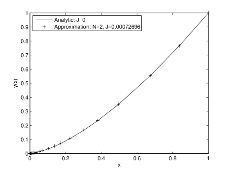
Figure 1: Analytic vs numerical solution to problem of Example 3.

Our numerical method works well, even in the case the minimizer is not a Lipschitz function.

Example 31.

An approximated solution to the problem considered in Example 4 can be obtained following exactly the same steps as in Example 30. Recall that the minimizer (11) to that problem is not a Lipschitz function. As before, one has $y(0)=0$ and the Caputo derivative coincides with the Riemann–Liouville derivative. We approximate the fractional problem using (39). Let ${}^{C}_{0}D_{x}^{\alpha}y(x)=u(x)$. Then (40) holds. In this case the variable $z(x)$ satisfies

$${z^{\prime}}(x)=\left(y(x)-\frac{x^{\alpha}}{\Gamma(\alpha+1)}\right)^{2}$$

and we approximate the fractional variational problem with the following classical one:

$$\begin{gathered}\tilde{J}(y)=\int_{0}^{1}[(u(x)-1)^{2}+z(x)]dx\longrightarrow\min\\ \begin{cases}{y^{\prime}}(x)=-AB^{-1}x^{-1}y(x)+\sum_{k=2}^{N}B^{-1}C_{k}x^{-k}v_{k}(x)+B^{-1}x^{\alpha-1}u(x)\\ {v^{\prime}}_{k}(x)=(1-k)x^{k-2}y(x),\qquad k=1,2,\ldots\\ {z^{\prime}}(x)=\left(y(x)-\frac{x^{\alpha}}{\Gamma(\alpha+1)}\right)^{2}\end{cases}\end{gathered}$$

subject to the boundary conditions $y(0)=0$, $z(0)=0$ and $v_{k}(0)=0$, $k=1,2,\ldots$ Setting $N=2$, the Hamiltonian is given by

$$H=-[(u(x)-1)^{2}+z(x)]+p_{1}(x)\left(-AB^{-1}x^{-1}y(x)+B^{-1}C_{2}x^{-2}v_{2}(x)+B^{-1}x^{\alpha-1}u(x)\right)\\ -p_{2}(x)y(x)+p_{3}(x)\left(y(x)-\frac{x^{\alpha}}{\Gamma(\alpha+1)}\right)^{2}.$$

The classical theory [36] tell us to solve the system

$$\left\{\begin{array}[]{ll}{y^{\prime}}(x)&=-AB^{-1}x^{-1}y(x)+B^{-1}C_{2}x^{-2}v_{2}(x)+\frac{1}{2}B^{-2}x^{2\alpha-2}p_{1}(x)+B^{-1}x^{\alpha-1}\\ {v^{\prime}_{2}}(x)&=-y(x)\\ {z^{\prime}}(x)&=(y(x)-\frac{x^{\alpha}}{\Gamma(\alpha+1)})^{2}\\ {p^{\prime}_{1}}(x)&=AB^{-1}x^{-1}p_{1}(x)+p_{2}(x)-2p_{3}(x)(y(x)-\frac{x^{\alpha}}{\Gamma(\alpha+1)})\\ {p^{\prime}_{2}}(x)&=-B^{-1}C_{2}x^{-2}p_{1}(x)\\ {p^{\prime}_{3}}(x)&=1\end{array}\right.$$ (44)

subject to boundary conditions

$$\begin{cases}y(0)=0\\ v_{2}(0)=0\\ z(0)=0\end{cases}\qquad\begin{cases}y(1)=\frac{1}{\Gamma(\alpha+1)}\\ p_{2}(1)=0\\ p_{3}(1)=0.\end{cases}$$ (45)

As done in Example 30, we solved (44)–(45) using the MATLAB^® built-in function bvp4c. The resulting graph for $y(x)$, together with the corresponding value of $J$, is given in Figure 2 in contrast with the exact minimizer (11).

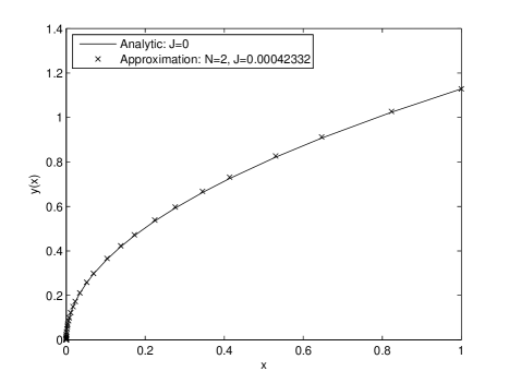
Figure 2: Analytic vs numerical solution to problem of Example 4.

References

- [1] O. P. Agrawal, A general formulation and solution scheme for fractional optimal control problems, Nonlinear Dynam. 38 (2004), no. 1-4, 323–337.
- [2] O. P. Agrawal, Generalized Euler-Lagrange equations and transversality conditions for FVPs in terms of the Caputo derivative, J. Vib. Control 13 (2007), no. 9-10, 1217–1237.
- [3] O. P. Agrawal, Fractional variational calculus in terms of Riesz fractional derivatives, J. Phys. A 40 (2007), no. 24, 6287–6303.
- [4] R. Almeida, A. B. Malinowska and D. F. M. Torres, A fractional calculus of variations for multiple integrals with application to vibrating string, J. Math. Phys. 51 (2010), no. 3, 033503, 12 pp. arXiv:1001.2722
- [5] R. Almeida, A. B. Malinowska and D. F. M. Torres, Fractional Euler-Lagrange differential equations via Caputo derivatives, in Fractional Dynamics and Control (eds: D. Baleanu, J. A. Tenreiro Machado, and A. Luo), Springer, in press.
- [6] R. Almeida and D. F. M. Torres, Hölderian variational problems subject to integral constraints, J. Math. Anal. Appl. 359 (2009), no. 2, 674–681. arXiv:0807.3076
- [7] R. Almeida and D. F. M. Torres, Isoperimetric problems on time scales with nabla derivatives, J. Vib. Control 15 (2009), no. 6, 951–958. arXiv:0811.3650
- [8] R. Almeida and D. F. M. Torres, Calculus of variations with fractional derivatives and fractional integrals, Appl. Math. Lett. 22 (2009), no. 12, 1816–1820. arXiv:0907.1024
- [9] R. Almeida and D. F. M. Torres, Leitmann’s direct method for fractional optimization problems, Appl. Math. Comput. 217 (2010), no. 3, 956–962. arXiv:1003.3088
- [10] R. Almeida and D. F. M. Torres, Necessary and sufficient conditions for the fractional calculus of variations with Caputo derivatives, Commun. Nonlinear Sci. Numer. Simulat. 16 (2011), no. 3, 1490–1500. arXiv:1007.2937
- [11] T. M. Atanackovic and B. Stankovic, On a numerical scheme for solving differential equations of fractional order, Mech. Res. Comm. 35 (2008), no. 7, 429–438.
- [12] N. R. O. Bastos, R. A. C. Ferreira and D. F. M. Torres, Discrete-time fractional variational problems, Signal Processing 91 (2011), no. 3, 513–524. arXiv:1005.0252
- [13] A. M. C. Brito da Cruz, N. Martins and D. F. M. Torres, Higher-order Hahn’s quantum variational calculus, Nonlinear Anal. (2011), in press. DOI: 10.1016/j.na.2011.01.015 arXiv:1101.3653
- [14] R. A. El-Nabulsi and D. F. M. Torres, Necessary optimality conditions for fractional action-like integrals of variational calculus with Riemann-Liouville derivatives of order , Math. Methods Appl. Sci. 30 (2007), no. 15, 1931–1939. arXiv:math-ph/0702099
- [15] R. A. El-Nabulsi and D. F. M. Torres, Fractional actionlike variational problems, J. Math. Phys. 49 (2008), no. 5, 053521, 7 pp. arXiv:0804.4500
- [16] R. A. C. Ferreira and D. F. M. Torres, Higher-order calculus of variations on time scales, in Mathematical control theory and finance (eds: A. Sarychev, A. Shiryaev, M. Guerra, and M. do R. Grossinho), 149–159, Springer, Berlin, 2008. arXiv:0706.3141
- [17] R. A. C. Ferreira and D. F. M. Torres, Isoperimetric problems of the calculus of variations on time scales, in Nonlinear Analysis and Optimization II (eds: A. Leizarowitz, B. S. Mordukhovich, I. Shafrir, and A. J. Zaslavski), Contemporary Mathematics, vol. 514, Amer. Math. Soc., Providence, RI, 2010, pp. 123–131. arXiv:0805.0278
- [18] R. A. C. Ferreira and D. F. M. Torres, Fractional -difference equations arising from the calculus of variations, Appl. Anal. Discrete Math. 5 (2011), in press. DOI: 10.2298/AADM110131002F arXiv:1101.5904
- [19] C. G. Fraser, Isoperimetric problems in the variational calculus of Euler and Lagrange, Historia Math. 19 (1992), no. 1, 4–23.
- [20] G. S. F. Frederico and D. F. M. Torres, A formulation of Noether’s theorem for fractional problems of the calculus of variations, J. Math. Anal. Appl. 334 (2007), no. 2, 834–846. arXiv:math/0701187
- [21] G. S. F. Frederico and D. F. M. Torres, Fractional conservation laws in optimal control theory, Nonlinear Dynam. 53 (2008), no. 3, 215–222. arXiv:0711.0609
- [22] G. S. F. Frederico and D. F. M. Torres, Fractional optimal control in the sense of Caputo and the fractional Noether’s theorem, Int. Math. Forum 3 (2008), no. 9-12, 479–493. arXiv:0712.1844
- [23] G. S. F. Frederico and D. F. M. Torres, Fractional Noether’s theorem in the Riesz-Caputo sense, Appl. Math. Comput. 217 (2010), no. 3, 1023–1033. arXiv:1001.4507
- [24] J. Gregory, Generalizing variational theory to include the indefinite integral, higher derivatives, and a variety of means as cost variables, Methods Appl. Anal. 15 (2008), no. 4, 427–435.
- [25] Z. D. Jelicic and N. Petrovacki, Optimality conditions and a solution scheme for fractional optimal control problems, Struct. Multidiscip. Optim. 38 (2009), no. 6, 571–581.
- [26] A. A. Kilbas, H. M. Srivastava and J. J. Trujillo, Theory and applications of fractional differential equations, North-Holland Mathematics Studies, 204, Elsevier, Amsterdam, 2006.
- [27] A. B. Malinowska and D. F. M. Torres, Delta-nabla isoperimetric problems, Int. J. Open Probl. Comput. Sci. Math. 3 (2010), no. 4, 124–137. arXiv:1010.2956
- [28] A. B. Malinowska and D. F. M. Torres, Generalized natural boundary conditions for fractional variational problems in terms of the Caputo derivative, Comput. Math. Appl. 59 (2010), no. 9, 3110–3116. arXiv:1002.3790
- [29] N. Martins and D. F. M. Torres, Calculus of variations on time scales with nabla derivatives, Nonlinear Anal. 71 (2009), no. 12, e763–e773. arXiv:0807.2596
- [30] N. Martins and D. F. M. Torres, Generalizing the variational theory on time scales to include the delta indefinite integral, submitted.
- [31] K. S. Miller and B. Ross, An introduction to the fractional calculus and fractional differential equations, A Wiley-Interscience Publication, Wiley, New York, 1993.
- [32] D. Mozyrska and D. F. M. Torres, Minimal modified energy control for fractional linear control systems with the Caputo derivative, Carpathian J. Math. 26 (2010), no. 2, 210–221. arXiv:1004.3113
- [33] D. Mozyrska and D. F. M. Torres, Modified optimal energy and initial memory of fractional continuous-time linear systems, Signal Process. 91 (2011), no. 3, 379–385. arXiv:1007.3946
- [34] T. Odzijewicz, A. B. Malinowska and D. F. M. Torres, Fractional variational calculus with classical and combined Caputo derivatives, Nonlinear Anal. (2011), in press. DOI: 10.1016/j.na.2011.01.010 arXiv:1101.2932
- [35] T. Odzijewicz and D. F. M. Torres, Fractional calculus of variations for double integrals, Balkan J. Geom. Appl. 16 (2011), in press. arXiv:1102.1337
- [36] L. S. Pontryagin, V. G. Boltyanskii, R. V. Gamkrelidze and E. F. Mishchenko, The mathematical theory of optimal processes, Translated from the Russian by K. N. Trirogoff; edited by L. W. Neustadt Interscience Publishers John Wiley & Sons, Inc. New York, 1962.
- [37] F. Riewe, Nonconservative Lagrangian and Hamiltonian mechanics, Phys. Rev. E (3) 53 (1996), no. 2, 1890–1899.
- [38] F. Riewe, Mechanics with fractional derivatives, Phys. Rev. E (3) 55 (1997), no. 3, part B, 3581–3592.
- [39] S. G. Samko, A. A. Kilbas and O. I. Marichev, Fractional integrals and derivatives, Translated from the 1987 Russian original, Gordon and Breach, Yverdon, 1993.
- [40] C. Tricaud and Y. Chen, An approximate method for numerically solving fractional order optimal control problems of general form, Comput. Math. Appl. 59 (2010), no. 5, 1644–1655.
- [41] B. van Brunt, The calculus of variations, Universitext, Springer, New York, 2004.