Clouds and the Faint Young Sun Paradox

Zusammenfassung

We investigate the role which clouds could play in resolving the Faint Young Sun Paradox (FYSP). Lower solar luminosity in the past means that less energy was absorbed on Earth (a forcing of ${-}$50 W m^-2 during the late Archean), but geological evidence points to the Earth being at least as warm as it is today, with only very occasional glaciations. We perform radiative calculations on a single global mean atmospheric column. We select a nominal set of three layered, randomly overlapping clouds, which are both consistent with observed cloud climatologies and reproduce the observed global mean energy budget of Earth. By varying the fraction, thickness, height and particle size of these clouds we conduct a wide exploration of how changed clouds could affect climate, thus constraining how clouds could contribute to resolving the FYSP. Low clouds reflect sunlight but have little greenhouse effect. Removing them entirely gives a forcing of ${+}$25 W m^-2 whilst more modest reduction in their efficacy gives a forcing of ${+}$10 to ${+}$15 W m^-2. For high clouds, the greenhouse effect dominates. It is possible to generate ${+}$50 W m^-2 forcing from enhancing these, but this requires making them 3.5 times thicker and 14 K colder than the standard high cloud in our nominal set and expanding their coverage to 100% of the sky. Such changes are not credible. More plausible changes would generate no more that ${+}$15 W m^-2 forcing. Thus neither fewer low clouds nor more high clouds can provide enough forcing to resolve the FYSP. Decreased surface albedo can contribute no more than ${+}$5 W m^-2 forcing. Some models which have been applied to the FYSP do not include clouds at all. These overestimate the forcing due to increased CO_2 by 20 to 25% when $p\chem{CO_{2}}$ is 0.01 to 0.1 bar.

Earth received considerably less energy from the Sun early in Earth’s history than today; ca. 2.5 Ga (billion years before present) the sun was only 80% as bright as today. Yet the geological evidence suggests generally warm conditions with only occasional glaciation. This apparent contradiction is known as the Faint Young Sun Paradox (FYSP, Ringwood, 1961; Sagan and Mullen, 1972). A warm or temperate climate under a faint sun implies that Earth had either a stronger greenhouse effect or a lower planetary albedo in the past, or both. In this study, we focus on the role of clouds in the FYSP. We both examine how their representation in models affects calculations of changes in the greenhouse effect, and constrain the direct contribution that changing clouds could make to resolving the FYSP.

Clouds have two contrasting radiative effects. In the spectral region of solar radiation (shortwave hereafter) clouds are highly reflective. Hence clouds contribute a large part of Earth’s planetary albedo (specifically the Bond albedo, which refers to the fraction of incident sunlight of all wavelengths reflected by the planet). In the spectral region of terrestrial thermal radiation (longwave hereafter), clouds are a strong radiative absorber, contributing significantly to the greenhouse effect. Cloud absorption is largely independent of wavelength (they approximate to “grey” absorbers), in contrast to gaseous absorbers which absorb only in certain spectral regions corresponding to the vibration–rotation lines of the molecules.

Despite the obvious, first-order, importance of clouds in climate, it has become conventional to omit them in models of early Earth climate and use instead an artificially high surface albedo. As described by Kasting et al. (1984):

Clouds are not included explicitly in the model; however, their effect on the radiation balance is accounted for by adjusting the effective albedo to yield a mean surface temperature of 288 K for the present Earth. The albedo is then held fixed for all calculations at reduced solar fluxes. $\ldots$we feel that the assumption of constant albedo is as good as can be done, given the large uncertainties in the effect of cloud and ice albedo feedbacks.

In effect, the surface is whitewashed in lieu of putting clouds in the atmosphere. This assumption has been used extensively in the models from Jim Kasting’s group (Kasting et al., 1984; Kasting and Ackerman, 1986; Kasting, 1987, 1988; Kasting et al., 1993; Pavlov et al., 2000, 2003; Kasting and Howard, 2006; Haqq-Misra et al., 2008), which, together with parametrisations and results based on these models (for example, Kasting et al., 1988; Caldeira and Kasting, 1992a, b; Kasting et al., 2001; Kasting, 2005; Tajika, 2003; Bendtsen and Bjerrum, 2002; Lenton, 2000; Franck et al., 1998, 2000; von Bloh et al., 2003a, b; Lenton and von Bloh, 2001; Bergman et al., 2004) have dominated early Earth palaeoclimate and other long term climate change research for the last two and a half decades. The validity of this method has not previously been tested.

Whilst Kasting’s approach is that changes to clouds are so difficult to constrain that one cannot justifiably invoke them to resolve the FYSP, others are more bold. Some recent papers have proposed cloud-based resolutions to the FYSP.

Rondanelli and Lindzen (2010) focus on increasing the warming effect of high clouds, finding that a total covering of high clouds which have been optimised for their warming effect could give a late Archean global mean temperature at freezing without increasing greenhouse gases. To justify such extensive clouds, they invoke the “iris” hypothesis (Lindzen et al., 2001) which postulates that cirrus coverage should increase if surface temperatures decrease (this hypothesis has received much criticism, e.g. Hartmann and Michelsen, 2002; Chambers et al., 2002).

Rosing et al. (2010) focus on decreasing the reflectivity of low level clouds so that the Earth absorbs more solar radiation. To justify this, they suggest that there was no emission of the important biogenic cloud condensation nuclei (CCN) precursor dimethyl sulphide (DMS) during the Archean and, consequently, clouds were thinner and had larger particle sizes.

We note that both Rondanelli and Lindzen (2010) and Rosing et al. (2010) predict early Earth temperatures substantially below today’s, which we do not consider a satisfactory resolution of the FYSP.

Shaviv (2003) and Svensmark (2007) proposes less low-level cloud on early Earth due to fewer galactic cosmic rays being incident on the lower troposphere. The underlying hypothesis is of a correlation between galactic cosmic ray incidence and stratus amount, through CCN creation due to tropospheric ionization (Svensmark and Friis-Christensen, 1997; Svensmark, 2007). This has received extensive study in relation to contemporary climate change and has been refuted (e.g. Sun and Bradley, 2002; Lockwood and Fröhlich, 2007; Kristjánsson et al., 2008; Bailer-Jones, 2009; Calogovic et al., 2010; Kulmala et al., 2010, and references therein).

In this study, we comprehensively asses how the radiative properties of clouds, and changes to these, can affect the FYSP. First, we explicitly evaluate how accurate cloud-free calculations of changes in the greenhouse effect are with respect to atmospheres with clouds included. We do this by considering a very wide range of cloud properties within a single global mean atmospheric column, finding a case study which matches Earth’s energy budget, then comparing the effect of more greenhouse gas in this column to a cloud-free calculation. Second, we conduct a very wide exploration of how changing clouds could directly influence climate. We vary fraction, thickness, height and particle size of the clouds and vary surface albedo. We do not advocate any particular set of changes to clouds. Rather, constraints on what direct contribution clouds can make towards resolving the FYSP emerges from our wide exploration of the phase space.

The heyday of clouds in 1-D models was the 1970s and 1980s. Improvements in radiative transfer codes and computational power over the last 30 years allow us to contribute new insight to the problem, in particular by widely exploring phase-space. Nonetheless, these classic papers retain their relevence and are instructive as to how one might treat clouds in such simple models (e.g. Schneider, 1972; Reck, 1979; Wang and Stone, 1980; Stephens and Webster, 1981; Charlock, 1982). With specific relevance to the FYSP, Kiehl and Dickinson (1987) included clouds in their model of methane and carbon dioxide warming on early Earth, and calculated radiative forcings from some changed cloud cases (our results here agree with this older work). Rossow et al. (1982) considered cloud feedbacks for early Earth.

Regarding whether a cloud-free model will correctly calculate the increased greenhouse effect with increases gaseous absorbers, we hypothesise that it will lead to an overestimation in the efficacy of enhanced greenhouse gases. In the absence of clouds, the broadest range of absorption is due to water vapour. However, whilst water vapour absorbs strongly at shorter and longer wavelengths, it absorbs weakly between 8 and 15 μm. This region of weak absorption is known as the water vapour window. It is coincident with the Wein peak of Earth’s surface thermal emission at 10 μm. Thus the water vapour window permits a great deal of surface radiation to escape to space unhindered. Other greenhouse gases – and clouds – do absorb here, so are especially important to the greenhouse effect. With clouds absorbing some fraction of the radiation at all wavelengths, the increase in absorption with increased greenhouse gas concentration would be less than if clouds were absent. Therefore, we think that a cloud-free model would overestimate increased gaseous absorption with increased greenhouse gas abundance and underestimate the greenhouse gas concentrations required to keep early Earth warm.

Comparison of cloudy and cloud-free radiative forcings in the context of anthropogenic climate change (Pinnock et al., 1995; Myhre and Stordal, 1997; Jain et al., 2000) supports our hypothesis. For CO_2, a clear-sky calculation overestimates the radiative forcing by 14%. For more exotic greenhouse gases, which are optically thin at standard conditions (CFCs, CCs, HCFCs, HFCs, PFCs, bromocarbons, iodocarbons), clear-sky calculations overestimate radiative forcing by 26–35%. CH_4 and N_2O are intermediate; their clear-sky radiative forcings are overestimated by 29% and 25%, respectively (Jain et al., 2000).

A roadmap of our paper is as follows. In Sect. 1 we describe our general methods, verification of the radiative transfer scheme and the atmospheric profile we use. In Sect. 2 we deal specifically with the development of a case study of three cloud layers representing the present climate and the model sensitivity to this. In Sect. 3 we compare cloudy and cloud-free calculations of the forcing from increased greenhouse gas concentration. In Sect. 4 we explore what direct forcing clouds could impart, and in section 5 we evaluate the aforementioned cloud-based hypotheses for resolving the FYSP.

1 Methods

1.1 Overview

Using a freely available radiative transfer code, we develop a set of cloud profiles for single-column models which is in agreement both with cloud climatology and the global mean energy budget. This serves as the basis for comparison of radiative forcing with a clear sky model and with changed cloud properties.

1.2 Radiative forcing

In work on contemporary climatic change, extensive use is made of radiative forcing to compare the efficacy of greenhouse gases (e.g. Forster et al., 2007). This is defined as the change in the net flux at the tropopause with a change in greenhouse gas concentration, calculated either on a single fixed temperature–pressure profile or a set of fixed profiles and in the absence of climate feedbacks. Surface temperature change is directly proportional to radiative forcing, with a radiative forcing of approximately 5 W m^-2 being required to cause a surface temperature change of 1 K (see Fig. 7 of Goldblatt et al., 2009b). Note that the tropopause must be defined as the level at which radiative heating becomes the dominant diabatic heating term (Forster et al., 1997), i.e. the lowest level at which the atmosphere is in radiative equilibrium.

We base all our analyses on radiative forcings here. As we make millions of radiative transfer code evaluations, saving in computational cost from comparing radiative forcings rather than running a radiative-convective climate model is significant, and facilitates the wide range of comparisons presented.

1.3 Global Annual Mean atmosphere

Tabelle 1: GAM profile at levels (layer boundaries). Note that the tropopause is at 100 hPa.

Pressure	Altitude	Temperature	Water vapour	Ozone
(Pa)	(km)	(K)	(g/kg)	(ppmv)
10	64.739	230.00	0.0036	1.080
20	59.912	245.61	0.0036	1.384
30	56.951	252.88	0.0036	1.626
50	53.114	260.00	0.0036	1.974
100	47.763	266.29	0.0035	2.600
200	42.393	260.33	0.0033	5.484
300	39.339	254.31	0.0032	6.810
500	35.612	243.24	0.0032	7.242
1000	30.842	228.11	0.0031	7.490
2000	26.290	222.10	0.0030	6.169
3000	23.671	218.71	0.0029	4.780
5000	20.445	212.59	0.0026	2.250
10000	16.204	206.89	0.0023	0.516
15000	13.727	211.83	0.0048	0.344
20000	11.914	219.01	0.0153	0.160
25000	10.461	225.87	0.0456	0.122
30000	9.237	233.27	0.1852	0.089
35000	8.168	240.52	0.3751	0.070
40000	7.215	247.19	0.6046	0.058
45000	6.352	253.27	0.8866	0.051
50000	5.562	258.62	1.2365	0.047
55000	4.834	263.15	1.6525	0.045
60000	4.159	267.14	2.1423	0.045
65000	3.529	270.73	2.7049	0.044
70000	2.938	274.00	3.3366	0.042
75000	2.381	277.05	4.1602	0.039
80000	1.855	279.84	5.2152	0.035
85000	1.356	282.28	6.3997	0.033
90000	0.882	284.08	7.8771	0.032
95000	0.431	285.85	9.5702	0.031
100000	0.000	289.00	11.1811	0.031

We perform all our radiative transfer calculations on a single Global Annual Mean (GAM) atmospheric profile (Table 1). This is based on the GAM profile of Christidis et al. (1997) with some additional high altitude data from Jain et al. (2000). Surface albedo is set as 0.125 (Trenberth et al., 2009). For standard conditions we use year 2000 gas compositions: 369 ppmv CO_2, 1760 ppbv CH_4 and, 316 ppbv N_2O. We use present day oxygen and ozone compositions throughout the work. Whilst comparisons without these might be interesting, they would necessitate using a different temperature profile in order to be self consistent. This would significantly complicate our methods, so no such calculations are performed. For solar calculations, we use the present solar flux and a zenith angle of 60.

Calculating radiative forcings on a single profile does introduce some error relative to using a set of profiles for various latitudes (Myhre and Stordal, 1997; Freckleton et al., 1998; Jain et al., 2000). However, as this is a methodological paper concerning single column radiative-convective models, it is the appropriate approach to take here.

1.4 Radiative transfer code and verification

We use the Atmosphere Environment Research (AER) Rapid Radiative Transfer Model (RRTM, Mlawer et al., 1997; Clough et al., 2005), longwave version 3.0 and shortwave version 2.5, which are available from http://rtweb.aer.com (despite different version numbers, these were both the most recent versions at the time of the research). RRTM has been parameterised for pressures between 0.01 and 1050 hPa and for temperatures deviating no more than 30 K from the standard mid-latitude summer (MLS) profile. We have verified that the GAM profile we use is within this region of pressure-temperature space. The cloud parameterisations in RRTM which we select follow Hu and Stamnes (1993) for water clouds and Fu et al. (1998) for ice clouds.

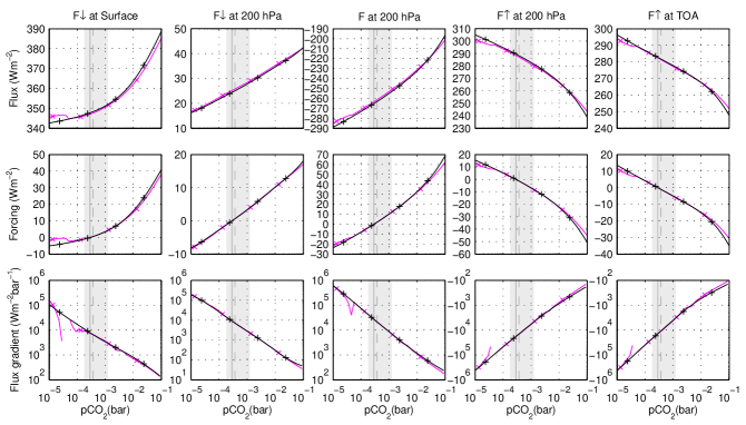
Abbildung 1: RRTM performance for CO_2 for each flux and each level. Colours (online only) and markers are: black ${+}$ for LBLRTM, magenta ${\times}$ for RRTM. Shaded areas are range from Quaternary minimum (180 ppmv) to SRES maximum (1248 ppmv) concentration. Grey lines in these areas are solid for pre-industrial (287 ppmv) and dashed for year 2000 (369 ppmv) concentrations.

RRTM has been designed primarily for contemporary atmospheric composition. Our intended use is for different atmospheric composition (higher greenhouse gas concentrations), so it is necessary for us to independently test the performance of the model under these conditions (Collins et al., 2006; Goldblatt et al., 2009b). Following the approach of Goldblatt et al. (2009b) we directly compare longwave clear sky radiative forcings from RRTM to the AER Line-by-Line Radiative Transfer Model (LBLRTM, Clough et al., 2005). These runs are done on a standard Mid-Latitude Summer (MLS) profile (McClatchey et al., 1971; Anderson et al., 1986) to take advantage of the large number of computationally expensive LBLRTM runs performed by Goldblatt et al. (2009b). Performance of the codes is evaluated at three levels: the top of the atmosphere (TOA), the MLS tropopause at 200 hPa and the surface. Upward and downward fluxes are considered separately. The surface is taken to be a black body, so the upward flux depends only on temperature ($F_{\mathrm{lw,surf}}^{\uparrow}=\sigma T_{*}^{4}$). The downward longwave flux at the TOA is zero. Neither vary with greenhouse gas concentrations, so changes in the net flux at these levels depends on one radiation stream only. At the tropopause the net flux is the sum of the two streams. It is defined positive downwards,

$$F_{\rm lw}=F_{\rm lw}^{\downarrow}-F_{\rm lw}^{\uparrow}{}\,.$$ (1)

In addition to the radiative flux, we show (Fig. 1) the forcing

$$\mathbb{F}_{\rm lw}=F_{\rm lw}-F_{\rm lw,std}{}\,,$$ (2)

where $F_{\rm lw,std}$ is the flux at preindustrial conditions and the flux gradient (change of flux with changing gas concentration)

$$\frac{\partial F}{\partial X}\approx\frac{\Delta F}{\Delta X}=\frac{F_{i+1}-F_{i}}{X_{i+1}-X_{i}}{}\,,$$ (3)

where $F_{i}$ is the flux at gas concentration $X_{i}$ (Goldblatt et al., 2009b).

Our focus is on comparison of cloudy to cloud-free profiles within RRTM, so we do not need high accuracy calculations of early Earth radiative forcings. We can therefore use rather relaxed and qualitative thresholds for acceptable model performance relative to LBLRTM: we require continuous and monotonic response to changing greenhouse gas concentration (no saturation), the forcing should be smooth and monotonic and divergence from the LBLRTM flux gradient should be limited. For CO_2, RRTM forcing is not smooth or monotonic below $p\chem{CO_{2}}{=}10^{-4}$ bar so this region is excluded (see Fig. 1). CO_2 concentrations up to $p\chem{CO_{2}}{=}10^{-1}$ bar are used, though there is some underestimation of radiative forcing by RRTM above $p\chem{CO_{2}}{=}10^{-2}$ bar. Also, collision-induced absorption (absorption due to forbidden transitions) becomes important at $p\chem{CO_{2}}\sim 0.1$ bar but coefficients for these are not included in the HITRAN database on which both RRTM and LBLRTM absorption coefficients are based. Therefore, it is emphasised that the radiative forcings presented here for high CO_2 will be underestimates, but valid for intra-comparison.

The comparison of RRTM to LBLRTM (Fig. 1) is only for the purpose of validating clear sky radiative forcing in the context of this methodological study. We have undoubtedly used RRTM outside its design range. This is not intended as an assessment of its use for the contemporary atmosphere or for anthropogenic climate change.

2 Cloud representation and model tuning

2.1 Practical problems and observational guidance

Generation of an appropriate cloud climatology for this work is not straightforward. Two fundamental problems are shortcomings in available cloud climatologies and averaging to a single profile. Concerning climatologies, the problem is one of observations: surface observers will see the lowest level cloud only, satellites will see the highest level of cloud only. Radiosondes are cloud penetrating and cloud properties may be inferred from measured relative humidity, but the spatial and temporal coverage of radiosonde stations is limited. See Wang et al. (2000) and Rossow et al. (2005) for extensive discussion of what progress can be made. Similarly, radar can profile clouds, but such observations are sparse. Concerning averaging, the dependence of the global energy budget on cloud properties is expected to be non-linear: one should not expect that a linear average of global cloud physical properties would translate into a set of clouds whose radiative properties would give energy balance in a single column. Nonetheless, available temporally and spatially averaged data for cloud properties can guide how clouds should be represented in the model.

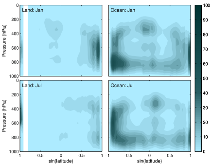
Abbildung 2: Average cloud fraction with altitude following Rossow et al. (2005, and W. Rossow, personal communication, 2009), for January and July, land and ocean. White areas are where there is either no land (the Southern and Arctic Oceans) or no ocean (Antarctica).

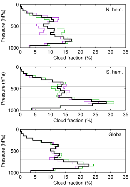
Abbildung 3: Average cloud fraction with altitude following Rossow et al. (2005, and W. Rossow, personal communication, 2009). (a) Northern Hemisphere. (b) Southern Hemisphere and (c) global for January (green), July (purple) and mean (black). Grey horizontal lines separate high, mid- and low-level clouds.

Rossow et al. (2005) deduce zonally-averaged cloud fraction profiles using a combination of International Satellite Cloud Climatology Program (ISCCP) and radiosonde data (Fig. 2). The existence of three distinct cloud layers and the pressure levels of these are immediately apparent when averaging the data meridionally (Fig. 3). Following Rossow and Schiffer (1999), we divide the clouds into three groups, with divisions at 450 and 700 hPa. “Low” cloud coresponds to cumulus, stratocumulus and stratus clouds. “Mid” level clouds correspond to altocumulus, altostratus and nimbostratus. “High” clouds correspond to cirrus and cirrostratus. Absolute cloud fractions cannot be extracted directly from these data as information on how the clouds overlap is lost in temporal and spatial averaging. A simple approach to give indicative values is to assume either maximum or random overlap within each group (high, middle and low), then to scale these cloud amounts by a constant such that randomly overlapping the three groups gives the IPCC mean global cloud fraction of 67.6% (Rossow and Schiffer, 1999). Maximum and random overlap within groups give cloud fractions $[f_{\rm high},f_{\rm mid},f_{\rm low}]{=}[0.24,0.25,0.43]$ and $[f_{\rm high},f_{\rm mid},f_{\rm low}]{=}[0.25,0.29,0.39]$, respectively.

Averaged cloud optical thickness or water paths are more difficult to constrain, as they are not directly available from the Rossow et al. (2005) data set . We proceed with ISCCP data only. Rossow and Schiffer (1999) report water paths of $[\,\mathcal{W}_{\rm high},\mathcal{W}_{\rm mid},\mathcal{W}_{\rm low}]{=}[23,60,51]$ g m^-2. ISCCP data are from downward looking satellite data only and overlap is not accounted for. Whilst the low cloud value will indicate low clouds only, high and mid level cloud values may include opacity contributions from the lower clouds which they obscure (see Fig. 2). Hence these water paths are indicative only.

Using fine resolution spatially and temporally resolved data would help resolve these issues. However, to do so would be beyond the scope of this work and, we feel, it is beyond what is necessary to address the first-order questions which are the subject of this paper.

2.2 Development of cloud profiles

We need to develop a set of cloud profiles which appropriately represents Earth’s cloud and energy budget climatologies. By necessity, we shall need to simplify cloud properties, tune our model clouds and consider sensitivity of the model energy budget to these clouds.

Even with the assumption that each cloud is homogeneous, each of our three cloud layers is represented by a cloud base and top, water path, liquid:ice ratio, and effective particle sizes for liquid and ice particles, giving 6 degrees of freedom for each cloud. With three layers, there are eight permutations for overlap, contributing another 7 degrees of freedom for the fractional coverage. A total of 25 degrees of freedom is clearly impossible to explore fully. As a necessary simplification, we fix the cloud base and top, take clouds to be either liquid (low and mid clouds) or ice (high clouds) and fix the particle size (following Rossow and Schiffer, 1999). We assume that cloud layers are randomly overlapped, so each cloud layer can be represented by a single fraction from which the overlap is calculated (many GCMs use a “maximum-random” overlap method where cloud fractions in adjacent layers are correlated; this is not relevant here as our discrete cloud layers are separated by intervals of clear sky, e.g. see Hogan and Illingworth, 2000).

Random overlap is easiest to explain for the case of two cloud levels (A and B), with cloud fractions $a$ and $b$. Fraction $ab$ of the sky would have both cloud layers, fraction $a(1{-}b)$ would only have level A clouds and fraction $(1{-}a)b$ would only have level B clouds, and fraction $(1{-}a)(1{-}b)$ would be cloud free. With three cloud layers, we have eight columns. Each column is evaluated separately in both longwave and shortwave spectral regions and the final single column is found as a weighted sum of these 16 evaluations. Different cloud fractions can be accounted for in this summation, reducing the number of RRTM evaluations needed.

Tabelle 2: Parameter values used in the large cloud tuning ensemble. Optical depth depends logarithmically on water path. Water path and cloud fraction are varied independently for each layer. Water paths range from optically thin to optically thick clouds (Curry and Webster, 1999) with 10 values. Cloud fractions range from 5% to 100% coverage with 20 cases. Effective radius is for water clouds (low and mid level) and generalised effective size is for ice clouds (high). There there are $10^{3}{\times}20^{3}{=}8{\times}10^{6}$ cases in total.

Fixed properties	High	Mid	Low
Cloud top (hPa)	300	550	750
Cloud base (hPa)	350	650	900
Liquid or ice	Ice	Liquid	Liquid
Effective radius (μm)	–	11	11
Generalised effective size (μm)	75	–	–
Variable properties	All layers
Water path (g m-2)	[$10^{0.4},10^{0.6},10^{0.8},\ldots,10^{2.2}$]
Cloud fraction	[0.05, 0.10, 0.15, …, 1.00]

For each cloud layer, cloud fraction and water path are varied widely whilst the other four parameters are fixed (Table 2). In all of the resulting cloud cases, we run the radiative transfer code for both standard and elevated CO_2 levels (369 ppmv and 50 000 ppmv), giving 16 million runs in total.

We refer to model runs in which we include clouds in this way as including “real clouds”. This is meant in the sense that clouds are included in the radiative transfer code in a detailed and physically based manner. This is by contrast to previous models (e.g. Kasting et al., 1984), where clouds are represented non-physically by changing surface albedo.

2.3 Sensitivity experiment

For each cloud case that we have defined (the large ensemble, Table 2), we calculate the radiative forcing at the tropopause ($\mathbb{F}_{\rm trop}$), to which change in surface temperature is proportional. Radiative forcing is the change in net flux (here with increasing $\chem{CO_{2}}$):

$$\mathbb{F}_{\rm trop}=F_{\rm[trop,high\chem{CO_{2}}]}-F_{\rm[trop,std\chem{CO_{2}}]}\,,$$ (4)

where $F$ in each case is the net flux as a sum of longwave and shortwave spectral regions and upward and downward streams of radiation:

$$F=(F_{\rm lw}^{\downarrow}-F_{\rm lw}^{\uparrow})+(F_{\rm sw}^{\downarrow}-F_{\rm sw}^{\uparrow})\,.$$ (5)

We consider two subsets of the large ensemble:

1. Cloud sets which give energy balance at the TOA. This is the most basic constraint on a possible climate. With $|F_{\rm TOA}|{<}5$ W m^-2, a subset of 1.0 million cases remains. A relatively large $|F_{\rm TOA,std\chem{CO_{2}}}|$ is allowed as variations in the water path are coarse, but it is corrected for by calculating radiative forcings so cannot bias the outcome.

2. Cloud sets which give energy balance at the TOA and are close to observed longwave and shortwave fluxes at the TOA (Trenberth et al., 2009). Constraints are $|F_{\rm TOA,std\chem{CO_{2}}}|{<}5$ W m^-2, $95{<}F\uparrow_{\rm TOA,SW,std\chem{CO_{2}}}{<}115$ W m^-2 and $227{<}F\uparrow_{\rm TOA,LW,std{CO_{2}}}{<}247$ W m^-2). This gives a subset of 36 985 cases.

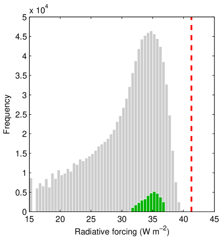
Abbildung 4: Histogram of radiative forcings from two subsets of cloud profiles. Cloud sets which give energy balance at the TOA (subset 1) in light grey, cloud sets which give energy balance at the TOA and are close to observed longwave and shortwave fluxes at the TOA superimposed darker (green online). Dashed vertical line (red online) shows radiative forcing cloud-free case for comparison.

The distribution of radiative forcings in these two subsets is shown relative to the cloud-free radiative forcing of 41.3 W m^-2 (Fig. 4). The maximum radiative forcing from subset 1 is 40.2 W m^-2; all physically plausible cloud sets give a smaller radiative forcing than a cloud-free model. Subset 2 – of cloud sets which give Earth-like climate – has a mean radiative forcing of 34.6 with a standard deviation of 1.3 W m^-2. The radiative forcing from the cloud-free case is 4.9 standard deviations above the mean radiative forcing from realistic, Earth-like, clouds.

Note that we perform these runs at the standard solar constant, as for all model runs herein. Given that $\chem{CO_{2}}$ is not a strong absorber in the shortwave spectral region, selecting a lower solar constant for the sensitivity experiment would not cause any noticeable change to Fig. 4. For example, using a solar flux 80% of the present value yields forcings different by 0.2 to 0.3 W m^-2.

2.4 Case study selection

Tabelle 3: Cloud properties used in case study. $f_{\rm total}{=}0.66$.

Property	High	Mid	Low
Cloud top (hPa)	250	500	700
Cloud base (hPa)	300	600	850
Cloud fraction	0.25	0.25	0.40
Water path (g m-2)	20	25	40
Liquid or ice	Ice	Liquid	Liquid
Generalised effective size ( μm)	75	–	–
Effective radius (μm)	–	11	11

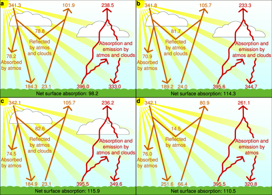
Abbildung 5: Comparison of global annual mean energy budgets: two estimates for contemporary climate, (a) Trenberth et al. (2009), based on a composite of data and (b) Zhang et al. (2004), from ISCCP-FD data, compared to models used in this paper, (c) case study with real clouds (d) cloud-free model.

As discussed, there are many problems associated with selecting a set of cloud profiles. However, the radiative forcings from CO_2 enhancement in all Earth-like cloud sets are closely grouped (Fig. 4) and the mean of these is significantly different from the cloud-free case. This justifies definition of a case study which can be used to represent Earth’s clouds. To do this from subset 2, we additionally constrain cloud fractions (each layer and the resultant total) and water paths of each layer to be close to climatological values, optimising for agreement with longwave and shortwave fluxes at the TOA. We found that, whilst shortwave fluxes could be found that were in good agreement with climatological values, the outgoing longwave fluxes were slightly too high in all cases from ensemble 2. Increasing the height of the clouds by 50 hPa gives a better fit for longwave fluxes. Case study cloud properties are given in Table 3 and the radiative outcome in Fig. 5c.

2.5 Cloud-free case

In order to compare calculated cloudy and cloud-free radiative forcings we need a cloud-free model as a comparison case. To generate this, we follow Kasting et al. (1984) and tune the surface albedo of the GAM profile to achieve energy balance at the top of the atmosphere for a clear sky profile. The required surface albedo is 0.264.

3 Real clouds and cloud-free model compared

First, consider the energy budget at standard conditions relative to observational climatology (Fig. 5). Our case study with real clouds (Fig. 5c) is in very good agreement with observational climatology (Fig. 5a,b). By contrast, almost all of the variable fluxes in the cloud-free model (Fig. 5d) are markedly different; omitting clouds means that the global energy budget is not properly represented. Overall in the cloud-free model, more absorption of solar radiation (only 81 W m^-2 of outgoing shortwave radiation is reflected rather than 106 W m^-2, a lower overall planetary albedo) is balanced by a weaker greenhouse effect (with an elevated outgoing longwave flux of 261 W m^-2 rather than 236 W m^-2 and depressed downward longwave at the surface).

Whilst no 1-D model can perfectly represent global climate, our real cloud case study, which is constrained by observational cloud climatology, gives good agreement with the observed energy budget. This justifies using it as an internal standard, against which the cloud-free model can be compared.

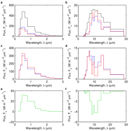
Abbildung 6: Comparison of spectrally resolved energy budgets in Real Cloud (RC, blue) and Cloud Free (CF, red) models. Black lines are for both cases. Green is for differences (CF${-}$RC). (a) $F\downarrow_{\rm SW}^{\rm TOA}$ for both cases in black, $F\uparrow_{\rm SW}^{\rm TOA}$ in colours. (b) $F\uparrow_{\rm LW}^{\rm surf}$ for both cases in black, $F\uparrow_{\rm LW}^{\mathrm{TOA}}$ in colours. (c) Absorption of solar radiation: $A{=}F\downarrow_{\rm SW}^{\rm TOA}{-}F\uparrow_{\rm SW}^{\rm TOA}$ (d) Greenhouse effect: $G{=}F\uparrow_{\rm LW}^{\rm surf}{-}F\uparrow_{\rm LW}^{\rm TOA}$ (e) Difference in solar absorption: $D_{A}{=}A({\rm CF}){-}A({\rm RC}$) (f) Difference in greenhouse effect: $D_{G}{=}G({\rm CF}){-}G({\rm RC}$).

Again at standard conditions, compare the spectrally resolved fluxes (Fig. 6). In the shortwave, the difference in adsorption between cloud-free and real cloud models (Fig. 6e) has the same shape as the Planck function of solar radiation (Fig. 6c). This is because the surface albedo is constant with wavelength by definition and the wavelength dependence of cloud scattering is weak. Rayleigh scattering is spectrally dependent (short wavelengths are preferentially scattered), but this is a small term (14.5 W m^-2 in the cloud-free case). By contrast, in the longwave, there is strong spectral dependence in the differences between the real cloud and cloud-free models. The cloud-free model has a weaker greenhouse effect than real clouds in the water vapour window region. Whilst other spectral regions are optically thick (with gaseous absorption by water vapour and carbon dioxide dominating) the water vapour window is optically thin and the cloud greenhouse is important.

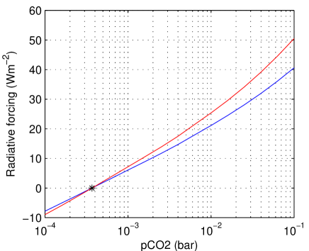
Abbildung 7: Radiative forcing with increasing $p\chem{CO_{2}}$. Real clouds in blue and cloud-free in red. Present $p\chem{CO_{2}}$ marked (✳).

Now consider the effect of changing CO_2 concentration (Fig. 7). Radiative forcing is strongly overestimated by the cloud-free model relative to our real cloud case study; to produce a given radiative forcing, twice as much CO_2 is needed with the real cloud case study than is indicated by the cloud-free model.

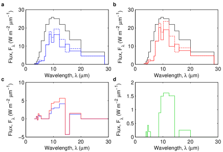
Abbildung 8: Comparison of spectrally resolved longwave forcings for increase from standard to 50 000 ppmv CO_2 in real cloud (RC, blue) and cloud-free (CF, red) models. Green is for differences in cases (CF${-}$RC) and black is for fluxes common between cases. (a) RC: $F\uparrow_{\rm LW}^{\rm surf}$ in black, $F\uparrow_{\rm LW}^{\rm TOA}$ dashed blue for standard CO_2 and solid blue for elevated CO_2; (b) CF: $F\uparrow_{\rm LW}^{\rm surf}$ in black, $F\uparrow_{\rm LW}^{\rm TOA}$ dashed red for standard CO_2 and solid red for elevated CO_2; (c) greenhouse forcing from increased CO_2: $\mathbb{G}{=}G({\rm High}\chem{CO_{2}}){-}G({\rm Std}\chem{CO_{2}}$) where $G{=}F\uparrow_{\rm LW}^{\rm surf}{-}F\uparrow_{\rm LW}^{\rm TOA}$; (d) difference in greenhouse forcing: $D_{\mathbb{G}}{=}\mathbb{G}({\rm CF}){-}\mathbb{G}({\rm RC}$).

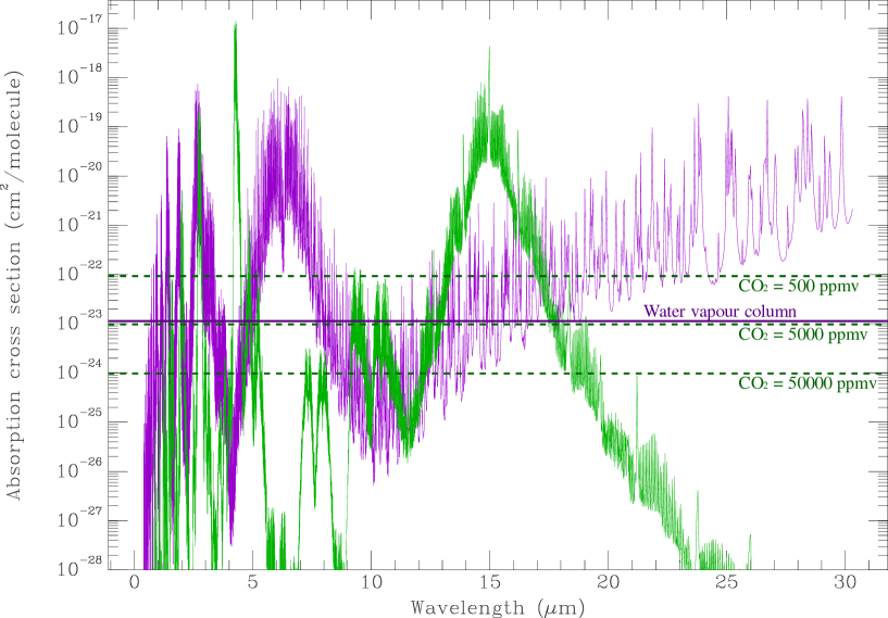
Abbildung 9: Absorption cross sections for CO_2 (green) and water vapour (purple) from HITRAN (shown at 900 hPa and 285 K). Horizontal lines indicate the cross section for which the gas has an optical depth of unity, solid purple for the GAM water vapour column, dashed green for various CO_2 concentrations. The column depth of the atmosphere is $2.1{\times}10^{25}$ molecules cm^-2.

The radiative forcing in the longwave is an order of magnitude larger than the radiative forcing in the shortwave region, so we focus on the longwave region when comparing spectrally resolved forcing (Fig. 8). The greenhouse effect with real clouds is stronger at standard conditions than the cloud-free model (inclusion of cloud greenhouse). However, the greenhouse forcing (increase in strength of the greenhouse effect), is larger in the cloud-free model. This is true across all bands where CO_2 imparts a greenhouse effect and is most important in the water vapour window. Here, the atmosphere is optically thin in the absence of clouds, so the effect of increasing CO_2 is large even though its absorption lines are weak (Fig. 9). With clouds, these regions will be optically thicker initially so increasing CO_2 has less of an effect.

At 15 μm, increasing CO_2 causes increased longwave emission. This is due to increased emission in the stratosphere and is therefore unaffected by tropospheric clouds.

Our GAM profile includes O_3 which absorbs at 9.5 μm and 9.7 μm. This would be absent in the anoxic Archean atmosphere, making the water vapour window optically thinner. The overestimation of forcing by the cloud-free model is, therefore, likely larger than suggested here and even more CO_2 would actually be needed to cause equivalent warming.

The other perturbation to consider is the change in incoming solar flux. The cloud-free model absorbs a higher proportion of the incoming solar flux (has a lower planetary albedo), so will have a proportionately larger response to changing solar flux. For an 20% decrease in solar flux, representative of the late Archean, the decrease in absorbed solar flux is 52.3 W m^-2 for the cloud-free model compared to 47.2 W m^-2 for the real-cloud case study. Taking the Archean to be lower solar flux but higher CO_2, this error is of opposite sign to the error in radiative forcing from increased CO_2 and around half the magnitude. Whilst these errors could be said to partially offset in these conditions, reliance on errors of opposing sign is not strong.

4 Variation of cloud and surface properties

The problem of cloud feedback on climate change is notoriously difficult. We do not attempt to address this in full; rather, we explore how variations in cloud amounts and properties could affect climate. In all cases here, our baseline case is the real cloud case study and we consider the radiative effect of changes in cloud or surface properties. As comparison values, if we increase or decrease the humidity in the model profile by 10% (50%), the radiative forcings are 1.7 W m^-2 (7.8 W m^-2) and ${-}$1.9 W m^-2 (${-}$11.2 W m^-2), respectively. A fainter sun in the late Archean is equivalent to a forcing of around ${-}$50 W m^-2 (assuming a planetary albedo of 0.3).

4.1 Surface albedo

In the cloud-free model, the use of a non-physical surface albedo means that real changes in surface albedo cannot be considered. This limitation is removed with explicit clouds. We limit discussion here to changes in surface albedo not from ice, though the use of a physically realistic surface with RC means that a parameterised ice-albedo feedback could be included in 1-D climate models, a significant improvement on the status quo.

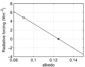
Abbildung 10: Radiative forcing with changed surface albedo. (✳) is the case study and ( $\circ$ ) is the end-member case of an ocean covered planet.

The surface albedo we use of 0.125 represents a weighted average of land (0.214) and ocean (0.090) albedos (Trenberth et al., 2009). Continental volume is generally thought to have increased over time, with perhaps up to 5% of the present amount at the beginning of the Archean and 20%–60% of the present amount by the end of the Archean (e.g. Hawkesworth and Kemp, 2006). In Fig. 10 we consider a range of variation of surface albedo appropriate for a changed land fraction. For the end-member case relevant to the Archean of a water-world, the radiative forcing is 4.8 W m^-2. Without land, relative humidity would likely be higher, contributing extra forcing.

4.2 Cloud fraction and water path

There are more clouds over ocean than land (Fig. 2). The zonally uninterrupted Southern Ocean is especially cloudy. One might therefore expect that when there was less land there would have been more cloud, and more still if there was a greater extent of zonally uninterrupted ocean. Comparison of the Northern and Southern Hemispheres of Earth (Fig. 3), the former having a higher land fraction, may be indicative of the minimum expected degree of variation. The Southern Hemisphere has 20–50% greater cloud fraction in each layer than the Northern Hemisphere.

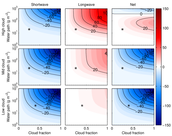
Abbildung 11: Cloud radiative forcing with cloud fraction and water path relative to no cloud in that layer. For each cloud layer, these properties are varied whilst the clouds in other layers remain fixed at the case study values, marked (✳). Particle sizes, ice/water ratio and height are as case study. Colour/contour scale is in W m^-2. For comparison, resolution of the late Archean FYSP would require a forcing of approximately 50 W m^-2.

We consider a wide range of water paths, from optically thin to thick clouds, and fractional cloud cover from zero to 1 for each cloud layer. In Fig. 11 we show the radiative forcing from these clouds relative to no cloud in the given layer. The competing shortwave and longwave effects of changing clouds can readily be seen. Increasing fraction or water path causes a negative forcing in the shortwave region (more reflection) but a positive forcing in the longwave (greenhouse effect). The greenhouse effect operates by absorption of thermal radiation emitted by a warm surface followed by emission at a lower temperature. Therefore the magnitude of changes in the greenhouse effect varies with cloud height, as higher clouds are colder. For low and mid level clouds, shortwave effects dominate and increasing cloud fraction or thickness will cause a net negative forcing (cooling the planet). For high clouds, shortwave and longwave effects are of similar magnitudes so the character of the net response is more complicated. For water paths less than 350 g m^-2, high clouds cause a net positive forcing (greenhouse warming the planet). The converse is true above 350 g m^-2, but such high water paths would typically correspond to deep convective clouds, not high clouds (cirrus or cirrostratus) (Rossow and Schiffer, 1999). Positive forcing is maximum for $\sim$70 g m^-2 high clouds.

4.3 Cloud particle size

Cloud particle size depends very strongly on the availability of cloud condensation nuclei (CCN). Whilst the global mean droplet size is 11 μm, this is biased by smaller droplets over land (average 8.5 μm), where there are more CCN than over the ocean (average 12.5 μm). Over the ocean, around half of CCNs are presently derived from oxidation products of biogenic dimethyl sulphide (DMS), especially sulphuric acid (there are various oxidation pathways of DMS (e.g. von Glasow and Crutzen, 2004), but only sulphuric acid can cause nucleation of new droplets (Kreidenweis and Seinfeld, 1988)). The climatic feedbacks involving DMS (Charlson et al., 1987) have been subject of long debate. Whilst DMS is prevalent today due to production by eukaryotes, other biogenic sulphur gases are produced by bacteria, in particular hydrogen sulphide (H_2S) and methyl mercaptan (CH_3SH) (Kettle et al., 2001). These will react chemically to form sulphates, which will provide CCN.

We do not delve deeply into CCN feedbacks here, but accept that various changes in the Earth system (e.g. atmospheric oxidation state, sulphur cycle, volcanic fluxes, biological fluxes) may well have changed CCN availability. Fewer CCN give larger cloud drops, which should both rain out quicker (so less cloud) and be less reflective. Conversely, more CCN give more extensive and more reflective clouds.

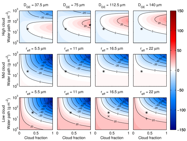
Abbildung 12: Change in net cloud radiative forcing with cloud particle size, across a range of cloud fractions and water paths. Particle size is varied for each layer independently (values in subplot titles), whilst all properties for other cloud layers remain as case study. The change is shown relative to the case study (so panels for $r_{\rm eff}{=}11$ μm and $D_{\rm GE}{=}75$ μm contain the same information as Fig. 11 net fluxes). Cloud fraction and water path for case study are marked (✳); values at the point of these markers are for changing particle size only, values elsewhere in each panel are for changing water path or fraction too. Markers (${\times}$) and (${+}$) refer to reduction in water path by factors of 2.2 and 3.7, respectively, for comparison to Rosing et al. (2010), as discussed in the text. Marker (✳) corresponds to the relatively thick and maximum extent clouds invoked by Rondanelli and Lindzen (2010). Colour/contour scale is in W m^-2.

We consider the effect of changing liquid droplet size by factors of 0.5, 1.5 and 2 relative to the case study ($r_{\rm eff}{=}11$ μm) and ice particle size by factors of 0.5, 1.5 and 1.87 relative to the case study ($D_{\rm GE}{=}75$ μm; the maximum of the parameterisation used is 140 μm). In Fig. 12, we show the net (shortwave plus longwave) radiative forcing from changing particle size for all water paths and fractions. The effect is strongest for low clouds. With no change to cloud fraction or water path, increasing $r_{\rm eff}$ by 50% gives a forcing of 7.5 W m^-2 and doubling $r_{\rm eff}$ gives a forcing of 10.4 W m^-2. Decreasing $r_{\rm eff}$ by 50% gives a forcing of ${-}$13.6 W m^-2.

Satellite observations of the modern ocean (Bréon et al., 2002) suggests a limit on how large droplet size actually becomes in nature. Particle size is rarely larger than 15 μm, even in the remotest and least productive regions of the ocean. Here, the DMS flux is low and remaining CCN derive from abiological sources (e.g. sea spray). $r_{\rm eff}{=}15$ μm can then be seen as the baseline case for lower CCN availability, corresponding to a 36% size increase relative to present day mean (20% relative to present day ocean).

If there was a larger CCN flux, the droplet size for clouds over land ($r_{\rm eff}{=}8.5$ μm, 23% less than mean) is an indicator of likely droplet size.

Larger droplets will rain out more effectively, but model representations of this feedback vary dramatically (Penner et al., 2006; Kump and Pollard, 2008). For the case of $r_{\rm eff}{=}17$ μm droplets over the ocean, Kump and Pollard (2008) choose a mid-strength assumption of this feedback, implying a decrease of water path by a factor of 2.2. This is marked (${\times}$) in the low cloud, 16.5 μm panel of Fig. 12; the radiative forcing is then 15.4 W m^-2, twice that of solely increasing droplet size. Clearly, an increased precipitation feedback is of first order importance and must be treated carefully in any model addressing the climatic effect of changed particle size.

4.4 Cloud height

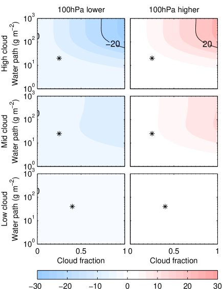
Abbildung 13: Cloud radiative forcing with changed cloud height relative to standard height clouds (see Fig. 11). Colour/contour scale is in W m^-2.

To test the sensitivity to cloud height, each cloud layer is raised or lowered 100 hPa and the forcing is calculated relative to the standard heights for all water paths and fractions. As temperature decreases with height, higher clouds emit at a lower temperature. It is this longwave effect which is dominant. There are only small changes in the shortwave effect, due to changed path length above the cloud (a greater path length means decreased insolation due to more Rayleigh scattering in the overlying atmosphere). In Fig. 13 we show only the net forcing. For the high clouds in the case study, which cover one-quarter of the sky and have a water path of 20 g m^-2, the effect of raising them is relatively small (2.8 W m^-2). There is a larger forcing from raising clouds which are thicker or cover more of the sky initially; the greater the radiative longwave effect of the cloud at its standard height, the greater the effect of changing it height would be.

Changes in the temperature–pressure structure of the atmosphere might have induced changes in clouds. The Archean atmosphere was anoxic and did not have an ozone layer (Kasting and Donahue, 1980; Goldblatt et al., 2006). Consequently, there would likely not have been a strong stratospheric temperature inversion, and deep atmospheric convection may have reached higher altitudes, where the atmosphere is colder. A major source of high clouds is detrainment of cirrus from deep convective clouds. Where detrainment is due to wind sheer, this could then result in higher clouds. Conversely, without an inversion a the tropopause, cumulonimbus incus (anvil shaped clouds) will not form. As the forcing from raising the high clouds in the case study is small, other climatic effects might be larger (loss of ozone as a greenhouse effect and lower stratospheric emission temperature). Also, the pressure of Archean atmosphere was likely not 1 bar. Not only was there no oxygen (0.21 bar today), but the nitrogen inventory was likely different (Goldblatt et al., 2009a). Varying pressure would have changed both the lapse rate and tropopause pressure (Goldblatt et al., 2009a).

5 Evaluating cloud-based proposals to resolve the Faint Young Sun Paradox

5.1 Increased cirrus

Rondanelli and Lindzen (2010) proposed that near total coverage of cirrus clouds could resolve the FYSP. Their proposed mechanism is that the planet would be colder and have lower sea surface temperatures, which would give more cirrus coverage (the controversial “iris” hypothesis of Lindzen et al., 2001), acting as a strong negative feedback on temperature. The first premise here, of colder temperatures, is contrary to the geological record; this suggests less frequent glaciation through the Archean and Proterozoic than in the Phanerozoic, not more. The second premise, of strong cloud feedback, is based on a statistical relationship for Earth’s tropics (Lindzen et al., 2001) the authenticity of which has been questioned (e.g. Hartmann and Michelsen, 2002; Chambers et al., 2002). Application to very cold temperatures requires an extreme and unverifiable extrapolation. Rondanelli and Lindzen (2010) describe the high level clouds they use as “thin cirrus”; we note that the clouds they use actually have twice the water path of our standard high clouds. In their sensitivity tests, using a thinner high level clouds gives a weaker effect.

Here, we consider what would be required of cirrus or other high level clouds for them to resolve the FYSP. Informed by the experiments above, we construct an optimum cirrus cloud for warming: relative to our case study we make it 3.5 times thicker (a water path of 70 g m^-2) and make it cover the whole sky, not just one-quarter (similar to the suggestion of Rondanelli and Lindzen, 2010). This gives a forcing of 29.0 W m^-2, insufficient to counter the ${\sim}$50 W m^-2 deficit from the FYSP. If, in addition, we raise the cloud by 100 hPa (base at 200 hPa, making the cloud 14 K colder) the total radiative forcing becomes 50.7 W m^-2.

In principle, high clouds can resolve the FYSP. In practice, the requirement for total high level cloud cover seems implausible and the requirement that the clouds are higher (colder) is difficult to justify. That it takes an extreme end-member case to provide only just enough forcing to resolve the FYSP suggests that resolution with enhanced cirrus only is not a strong hypothesis.

5.2 Decreased stratus

Rosing et al. (2010) propose that there were less CCN available in the Archean, due to lower DMS emissions prior to the oxygenation of the atmosphere and widespread occurrence of eukarya. They suggest an increase in droplet size from 12 μm to 20 or 30 μm. Even over unproductive regions of today’s oceans, the effective radius of cloud particles rarely exceeds 15 μm (Bréon et al., 2002), so it is difficult to see how such large effective radii could be justified. Larger droplets lead to more rain, so should make clouds thinner. To account for this, Rosing et al. (2010) arbitrarily decrease the liquid water path of their stratus clouds by a factor of 3.7, which is at the high end of likely decreases (Penner et al., 2006). Even with these very strong assumptions, their model temperature is continually below the present temperature before 2 Ga.

In our framework of radiative forcings, the effects of changing effective radius and cloud water path are shown in Fig. 12. For the strong but arguably plausible case (discussed in Sect. 4.3) of doubling the effective radius and decreasing water path by a factor of 2.2 gives a radiative forcing of 15.4 W m^-2. For the yet stronger case of doubling the effective radius from 11 μm to 22 μm and decreasing cloud water path by a factor of 3.7, the radiative forcing is 20.5 W m^-2. Removing low cloud entirely gives a forcing of 25.3 W m^-2. We therefore conclude that reducing stratus cannot by itself resolve the FYSP.

A separate hypothesis (Shaviv, 2003; Svensmark, 2007) proposes less stratus on early Earth due to fewer galactic cosmic rays being incident on the lower troposphere. The underlying hypothesis is of a correlation between galactic cosmic ray incidence and stratus amount, through CCN creation due to tropospheric ionization (Svensmark and Friis-Christensen, 1997; Svensmark, 2007). This hypothesis has been refuted (e.g. Sun and Bradley, 2002; Lockwood and Fröhlich, 2007; Kristjánsson et al., 2008; Bailer-Jones, 2009; Calogovic et al., 2010; Kulmala et al., 2010, and references therein): galactic cosmic rays cause the formation of at most 10% of CCNs and there is no correlation between galactic cosmic ray incidence and cloudiness. Also of note is that Shaviv (2003) requires a highly non-standard climate sensitivity to force his model. In the sensitivity test where he uses a more standard climate sensitivity, it results in a mean temperature $\sim 0^{\circ}$C during the Archean. Even if the underlying hypothesis had not been refuted, the same arguments as above would apply: plausible decreases in stratus are insufficient to resolve the FYSP.

When calculating radiative forcing from increased greenhouse gas concentrations, we find that omitting clouds leads to a systematic overestimate relative to models in which clouds are included in a physically based manner. With 0.1 bar CO_2 (the relevant quantity for a CO_2 based resolution to the Faint Young Sun Paradox in the late Archean) the overestimate of radiative forcing from modelling without clouds approaches 10 W m^-2 in our model, equivalent to the clear-sky forcing from 100 ppm CH_4. As the radiative transfer code we use underestimates forcing from CO_2 at this level, and we include O_3 in our profile, the difference between the real cloud case study and the cloud-free model here must be seen as a lower bound on the error from omitting clouds. For other greenhouse gases, especially those which absorb strongly in the water vapour window, the overestimation by a cloud-free model would likely be larger. This would affect calculations of the warming by methane and ammonia and of recently proposed Archean greenhouse gases, ethane (Haqq-Misra et al., 2008) and OCS (Ueno et al., 2009).

The question of what direct effect clouds might have is a more interesting and difficult one. We can address this best by considering what radiative forcing can be generated in both the shortwave and longwave spectral regions by changing cloud physical properties, and whether such changes in cloud physical properties can be justified.

For solar radiation (shortwave), low level stratus clouds have the greatest effect. Removing them from the model entirely gives a forcing of 25 W m^-2. Even this end-member falls short of the 50 W m^-2 that is needed to resolve the FYSP. A more plausible combination of reduced fraction and water path and increased droplet size would give a maximum forcing of 10–15 W m^-2. However, suitable justification for these changes does not come easily. Rosing et al. (2010) asserted that DMS fluxes would be low in the Archean, but there may well have been other biological and chemical sources for the sulphuric acid on which water condenses (DMS is a precursor to this). For example, methyl mercaptan is produced abundantly by bacteria (Kettle et al., 2001). Observations of clouds show that the effective radius rarely becomes larger that 15 μm (Bréon et al., 2002), which implies that regionally low CCN flux does not lead to very large droplets. If there were less land early in Earth’s history and more zonally uninterrupted ocean, one might expect there to be more cloud rather than less (similar to how there is greater cloud fraction in the Southern Hemisphere than the Northern Hemisphere). Also relating to low cloud, Shaviv (2003) and Svensmark (2007) contend that less galactic cosmic rays were incident on the troposphere during the Archean and this would have led to less stratus. However, the underlying hypothesis for this has been refuted.

For terrestrial radiation (longwave), high level clouds are most important as they are coldest (the greenhouse effect depends on the temperature difference between the surface and the cloud). The end member case is 100% coverage of high clouds which are optimised for their greenhouse effect, being both thicker and higher than our case study. Such an end member case gives a forcing of 50 W m^-2, which would just be sufficient to resolve the FYSP. However, physical justification for any of the required changes is lacking. Rondanelli and Lindzen (2010) invoke a controversial negative feedback of increased cirrus fraction with decreased temperature (the “iris” hypothesis of Lindzen et al., 2001), but a true resolution to the FYSP should give temperatures equal or higher than present. Thus, even if the “iris” hypothesis was correct, it would act to oppose warming. It is difficult to think of other mechanisms to make high clouds wider and thicker. Whether clouds should have been higher in the Archean may warrant more study. The absence of the strong stratospheric temperature inversion presently caused by ozone might contribute. However, without increase in fraction or cloud water path, the forcing will likely be less than 5 W m^-2.

The question then naturally arises: How should one model early Earth climate? Some would look first towards a general circulation model (GCM), in order to better represent the dynamics on which clouds depend. We disagree. Whilst dynamics are certainly important, it is unrealistic to think that in the near future clouds could be resolved in a global scale climate model applicable to palaeoclimate. Even in “high resolution” models used for anthropogenic global change, cloud processes are parameterised sub-grid scale. As one moves towards deep palaeoclimate research, one moves further from the present atmospheric state for which the model may have been designed and can be validated. A larger model therefore introduces greater, and harder to track, uncertainty. Considering what radiative forcing or warming a given mixture of greenhouse gases will impart is a first-order question, and one which should be answerable with a first-order model. A 1-D model is sufficient for this, but clouds must be included. The appropriate starting point would likely be a model with fixed cloud optical depth and fixed cloud top temperature (see, for example Reck, 1979; Wang and Stone, 1980). For any proposed change to clouds, very great attention is needed to the feasibility of the mechanism involved. To model these, one should probably look towards a cloud microphysics resolving model, coupled to appropriate models of CCN supply and chemistry.

A stronger greenhouse effect likely contributes the largest part of the forcing required to keep early Earth warm. It is important to remember, however, that the forcing from a greenhouse gas depends on the logarithm of its abundance. Thus, a modest forcing from clouds could have a large effect on how much of a greenhouse gas in needed; indicatively, a 10 W m^-2 from CO_2 requires a increase in concentration of a factor of 2 to 3. A large atmospheric CO_2 reservoir ($\sim 0.1$ bar) may be slow to accumulate, as geochemical processes (principally volcanic outgassing) contributing linearly to concentration, so any other forcings may be rather useful in resolving the FYSP.

In summary, it is necessary to include clouds in climate models if these are to be accurate. Resolution of the faint young sun paradox likely requires a combination of a few different warming mechanisms, including strong contributions from one or more greenhouse gases. Changed clouds could contribute warming, but this has yet to be justified – and cooling caused by cloud changes is equally possible. Future work will no doubt propose novel mechanisms to change clouds. We hope that the results presented here will facilitate quick and accurate look-up the climatic effect of such changes. Proposed cloud-based resolutions with only limited greenhouse enhancement are not plausible.