Geometry and Curvature of Spin Networks

Abstract

A measure for the maximum quantum information transfer capacity (ITC) between nodes of a spin network is defined, and shown to induce a metric on a space of equivalence classes of nodes for homogeneous chains with XX and Heisenberg couplings. The geometry and curvature of spin chains with respect of this metric are studied and compared to the physical network geometry. For general networks hierarchical clustering is used to elucidate the proximity of nodes with regard to the maximum ITC. Finally, it is shown how minimal control can be used to overcome intrinsic limitations and speed up information transfer.

I Introduction

Networks of interacting quantum particles — so-called spin-networks — are important for transferring and distributing quantum information between different parts of a larger system such as different quantum components on a chip [1]. Spin chains, linear arrangements of spins, for example, can play the role of classical wires connecting two parts, and branched networks allow the distribution of quantum information to different nodes. The way quantum information propagates through spin networks, however, is quite different from classical information flow due to quantum inference effects. In particular, quantum state transfer between the nodes of the network is limited by fundamental physical principles and perfect quantum state transfer is usually possible only in very special cases. Quantifying state transfer fidelities for spin networks is not easy in general, but for certain types of networks such as spin-$\frac{1}{2}$ particles with interactions of so-called XXZ type, for example, this problem can be reduced to the maximum probability for a single excitation to propagate from one node to another, which can be computed efficiently numerically, and in some cases analytically. Thus, for the respective spin networks, the latter is a basic measure for the maximum information transfer capacity (ITC) between different nodes. For certain types of simple networks such as homogeneous chains the maximum ITC is shown to induce a metric on a set of equivalence classes. We study the topology of simple networks with regard to this metric, showing that it differs substantially from the physical geometry. Networks with trivial physical geometry such as linear chains can have a surprisingly rich geometric structure including curvature. Analysis of the latter shows that spin chains appear to be Gromov-hyperbolic with regard to this maximum ITC metric but unlike classical hyperbolic networks their Gromov boundary appears to be a single point. For more complex networks the maximum ITC does not induce a metric but we can use hierarchical clustering to assess the proximity of nodes with regard to information transfer capacity. Again, the resulting cluster structures differ substantially from the neighborhood relations induced by the physical geometry of the network, showing that the latter is not very useful in assessing the maximum ITC between nodes in a network, unlike in the classical case. Finally, we consider how minimal control of a single node in the network allows us to change information flow in the network, effectively changing the information transfer capacities (and network “topology”), allowing us to achieve higher state transfer fidelities as well as generally speeding up the rate of information transfer.

II Information Transfer Capacity

The Hilbert space of spin networks with XXZ interactions can be decomposed into so-called excitation subspaces $\mathcal{H}=\oplus_{n=0}^{N}\mathcal{H}_{n}$, where $n$ is the number of excitations in the network, ranging from $0$ to $N$. If we denote the spin basis states by $|{\uparrow}\rangle$ and $|{\downarrow}\rangle$, taking the latter to denote the ground state, then the $0$-excitation subspace consists of a single state $|0\rangle:=|{\downarrow}\rangle\otimes\cdots\otimes|{\downarrow}\rangle$, while the one-excitation subspace consists of $N$ states $|n\rangle:=|{\downarrow}\rangle\otimes\cdots\otimes|{\uparrow}\rangle\otimes\cdots\otimes|{\downarrow}\rangle$, where the excitation $|{\uparrow}\rangle$ is in the $n$th position. Thus transferring a quantum state $|\psi\rangle=\cos(\theta)|{\downarrow}\rangle+e^{i\phi}\sin(\theta)|{\uparrow}\rangle$ from spin $m$ to $n$ is equivalent to transferring an excitation $|{\uparrow}\rangle$ from spin $m$ to $n$:

$$|\psi\rangle_{m} =\cos(\theta)|0\rangle+e^{i\phi}\sin(\theta)|m\rangle$$

$$\mapsto\cos(\theta)|0\rangle+e^{i\phi}\sin(\theta)|n\rangle=|\psi\rangle_{n},$$

where we used the shorthand $|\psi\rangle_{n}$ to denote a product state $|{\downarrow}\rangle\otimes|\psi\rangle\otimes|{\downarrow}\rangle$, whose $n$th factor is $|\psi\rangle$, all others being $|{\downarrow}\rangle$.

$$\begin{array}[]{llll}\hline\cr N&\mbox{vertices/equivalence classes}&\mbox{geometry}&\mbox{Distances}\\ \hline\cr 3&a=\{1,3\},b=\{2\}&\mbox{single edge}&\overline{ab}=0.81\\ 4&a=\{1,4\},b=\{2,3\}&\mbox{single edge}&\overline{ab}=0.32\\ 5&a=\{1,5\},b=\{2,4\},c=\{3\}&\mbox{triangle}&0.33=\overline{ac}=\overline{bc}>\overline{ab}=0.87\\ 6&a=\{1,6\},b=\{2,5\},c=\{3,4\}&\mbox{triangle}&0.48=\overline{ab}=\overline{cb}>\overline{ac}=0.36\\ 7&a=\{1,7\},b=\{2,6\},c=\{3,5\},d=\{4\}&\mbox{triangular pyramid}&\overline{ad}=\overline{bc}=\overline{cd}\gg\overline{ab}=\overline{bc}=\overline{ac}\\ 8&a=\{1,8\},b=\{2,7\},c=\{3,6\},d=\{4,5\}&\mbox{triangular pyramid}&\overline{ad}=\overline{bc}=\overline{cd}>\overline{ab}=\overline{bc}=\overline{ac}\\ 9&a=\{1,9\},b=\{3,7\},c=\{4,6\},d=\{2,8\},e=\{5\}&\mbox{4-simplex}&\overline{ab}=\overline{ac}=\overline{bc}<\overline{ad}=\overline{bd}=\overline{cd}\ll\overline{ae}=\overline{be}=\overline{ce}\\ 10&a=\{1,10\},b=\{2,9\},c=\{4,7\},d=\{5,6\},e=\{3,8\}&\mbox{4-simplex}&\overline{ab}=\overline{ac}=\overline{bc}<\overline{ad}=\overline{bd}=\overline{cd}<\overline{ae}=\overline{be}=\overline{ce}\\ \hline\cr\end{array}$$

TABLE I: ITC geometry of linear Heisenberg chains.

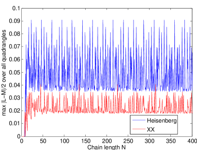
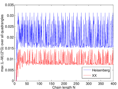
Figure 1: Chain length versus 4-point Gromov $\delta$ (left) and scaled 4-point Gromov $\delta$ (right). Scaled-Gromov $\delta$ remains below the upper bound singled out in [4], 4-point Gromov $\delta$ saturates at large chain length, revealing Gromov hyperbolic property. $G=L+M+S$ where $L$, $M$ and $S$ are the pairs of opposite diagonals of a quadrangle corresponding to the largest, medium and smallest length.

The probability that an excitation created at site $|i\rangle$ has propagated to site $|j\rangle$ after some time $t$ is given by

$$p(|i\rangle,|j\rangle,t)=|\langle j|e^{-\imath Ht}|i\rangle|^{2}$$ (1)

in the system of units where $\hbar=1$. The maximum of this probability $p(i,j)=\max_{t\geq 0}p(i,j,t)$, or a monotonic function thereof such as

$$d(i,j)=-\log p(i,j)$$ (2)

gives a measure for the maximum state transfer fidelity between two nodes in a spin network without control, quantifying the intrinsic capacity of a spin network for quantum state transfer tasks. It can be shown that

$$p(i,j) =\left|\langle i|e^{-\imath Ht}|j\rangle\right|=\left|\sum_{k}\langle i|v_{k}\rangle\langle v_{k}|j\rangle e^{-\imath\lambda_{k}t}\right|$$

$$\leq\sum_{k}\left|\langle i|v_{k}\rangle\langle v_{k}|j\rangle\right|,$$

where $H=\sum_{k=1}^{N}\lambda_{k}|v_{k}\rangle\langle v_{k}|$ is the eigendecomposition of the Hamiltonian operator $H$ of the network in the first excitation subspace $\mathcal{H}_{1}$. If the rescaled eigenvalues $\frac{\lambda_{1}}{\pi},\ldots,\frac{\lambda_{N}}{\pi}$ are rationally independent [2, Proposition 1.4.1] then it can be shown that for any $\epsilon>0$ there exists a $t_{\epsilon}>0$ such that $p_{\max}(i,j)-p(i,j,t_{\epsilon}))<\epsilon$, i.e., the maximum ITC is a tight bound and attainable in the limit.

III ITC Geometry & Curvature of Chains

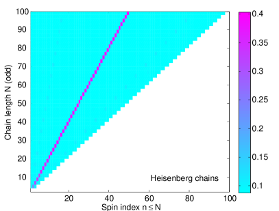
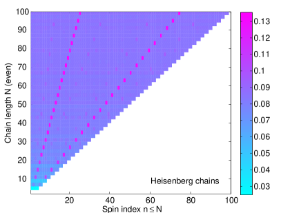
Figure 2: Inertia ($\alpha=2$) versus chain length plots for Heisenberg chains. For $N$ odd (left) the central node is a strong anti-gravity center. For $N$ even (right) there are weaker anti-gravity centers between end spins and middle (right). The inertia is symmetric about the central node as antipodal spins belong to the same equivalence class.

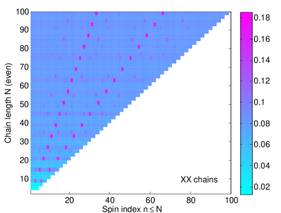
Figure 3: Inertia ($\alpha=2$) versus chain length plots for XX chains. For $N$ odd (left) the central node is a strong anti-gravity center and weaker anti-gravity centers exist for intermediate nodes. For $N$ (even) the anti-gravity centers are located between end and central spins. Again, the inertia is symmetric about the central node as antipodal spins belong to the same equivalence class.

Inspired by [3] we may hope that the maximum ITC measure $d(i,j)$ defined above can be shown to be a distance. $d(i,j)$ clearly satisfies $d(i,i)=0$ as $p(i,i)=1$, and we also have symmetry as obviously $p(i,j)=p(j,i)$. However, $d(i,j)$ can vanish for $i\neq j$ if $p(i,j)=1$, and in general we cannot expect the triangle inequality to hold. In special cases, however, such as for homogeneous chains with either XX or Heisenberg coupling, numerical exploration for systems up to 500 spins shows that the triangle inequality

$$D_{ijk}=d(i,k)+d(j,k))-d(i,j)\geq 0.$$ (3)

seems to be universally satisfied. This renders $d(i,j)$ a semi-distance, which induces a proper distance on a set of equivalence classes defined by identifying nodes with $d(i,j)=0$. Specifically, for Heisenberg or XX chain with uniform coupling the $N$ spins can be shown to form $\lceil\tfrac{N}{2}\rceil$ equivalence classes comprised of spins $n$ and $N+1-n$, which we shall denote by $n$ for $n=1,\ldots,\lceil N/2\rceil$ in a slight abuse of notation. On this set of equivalence classes the ITC measure $d(i,j)$ is a metric, and it is interesting to study the induced geometry of a spin chain with respect to the ITC metric, and how it differs from the physical network geometry. Table I gives the ITC geometry for Heisenberg chains up to $N=10$, showing that it is very different from the (trivial) physical geometry. A Heisenberg chain of length $N=7$, for instance, appears as a pyramid structure with an equilateral triangle as its base formed by the vertices $a=\{1,7\}$, $b=\{2,6\}$, $c=\{3,5\}$ and $d=\{4\}$ as its apex, where $n$ refers to the index of the spin in the chain. Chains up to length $N=8$ can be embedded in $\mathbb{R}^{3}$ but for longer chains higher-dimensional spaces are required. By Schoenberg’s theorem [5] the distances $d(i,j)$ can be realized in $\mathbb{R}^{d}$ if and only if the Gram matrix $G=(G_{ij})$ is positive semi-definite of rank $d$, where

$$G_{ij}=\tfrac{1}{2}\left(d(i,N)^{2}+d(j,N)^{2}-d(i,j)^{2}\right).$$ (4)

(This is equivalent to the Cayley-Menger matrix criterion of [6].) We numerically verified that the Gram matrix for both Heisenberg and XX chains is positive semi-definite for spins up to $N=500$. Analysis of the rank of the Gram matrix furthermore suggests that the dimension $d$ required to embed a chain of length $N$ is $\lceil\tfrac{N-2}{2}\rceil$ for both Heisenberg and XX chains. Note that Schoenberg’s theorem also applies to the geometric realisability of general spin networks and whether our ITC measure fulfills the triangle inequality.

To better understand the geometry for very long chains we analyze its curvature à la Gromov. From both the Gromov and the scaled-Gromov point of view [7] spin chain of both Heisenberg and XX coupling type appear hyperbolic. The strict Gromov point of view is displayed in Fig. 1(a) and the scaled-Gromov point of view is shown in Fig. 1(b). The Gromov property might appear to conflict with the Euclidean embeddability of the metric space made up by the clusters with the ITC metric, as the Bonk-Schramm [8] theorem says that Gromov negatively curved spaces are embeddable in hyperbolic space. However, some metric spaces are embeddable in both Euclidean and hyperbolic spaces, the most striking example being that of a complete graph with uniform edge weight, and spin chains with uniform couplings appear to fall into this category.

Classical communication networks, both wired [7, 9] and wireless [3], have been shown to be Gromov hyperbolic. Gromov hyperbolic spaces have a unique vertex that achieves the minimum inertia [10], the so-called gravity center

$$g=\arg\min_{i}I(i)=\arg\min_{i}\sum_{j}d^{\alpha}(i,j),\quad\alpha\geq 1.$$ (5)

Classical networks indeed show a point of minimum inertia, which can be interpreted as a congestion point [11]. Classical networks also have the property that their Gromov boundary in the asymptotic limit is a Cantor set [12]. Quite surprisingly, quantum networks differ from their classical counterparts in that they have points of maximum inertia, or anti-gravity centers, as shown in Figs 2 and 3 for Heisenberg and XX chains, respectively, and their Gromov boundary is a single point. The interpretation of the antigravity center is that the information flow in the network avoids this node, making it difficult to transfer excitation to and from it. It is interesting to note in this context that the distance between antipodal nodes is $0$, meaning that we can achieve state transfer fidelities arbitrarily close to $1$, i.e., near perfect state transfer between the ends of the chain of any length given sufficient time, while near perfect state transfer is never possible between any pair of nodes with $d(i,j)>0$, no matter how long we wait.

IV ITC “Topology” Of General Networks

The maximum transfer probability is also a useful measure for the maximum fidelity of quantum state transfer in general spin networks. Although it is in general no longer a metric, it can still be used as a similarity measure to define a hierarchical clustering. We use the pairwise clustering algorithm introduced in [13]. Pairs of nodes are grouped hierarchically into clusters in order of their similarity, and only those clusters whose elements are closer to each other than any element outside the cluster are preserved. If we define a relation

$$|a\rangle=_{\epsilon}|b\rangle:\Leftrightarrow d(|a\rangle,|b\rangle)<\epsilon$$ (6)

for nodes $|a\rangle$, $|b\rangle$, then these clusters are the equivalence classes of $=_{\epsilon}$ for a certain $\epsilon$. The cluster hierarchy reveals the closeness of the nodes in terms of information transfer.

For example, consider a network of 10 spins distributed in a square forming a general spin network as shown in Fig. 4. The positions of the spins are indicated by the blue dots. Taking the coupling strength $J(i,j)$ between spins $i$ and $j$ to be inversely proportional to the cube of the physical distance between the nodes, we compute the Hamiltonian of the network, assuming XX-coupling. We then diagonalize this Hamiltonian and compute the maximum transfer probabilities $p(i,j)$ and the associated $d(i,j)$, which are used as input for our clustering algorithm. The resulting hierarchical clustering structure is shown in Fig. 4. Different colours indicate clusters for different similarity levels; i.e. for clusters marked in the same colour there exists an $\epsilon$ for which these are the equivalence classes of $=_{\epsilon}$. Again, the example shows that the physical distance of the spins is not a good measure of their proximity in an quantum information transfer fidelity sense. For instance, spin $9$ is physically closer to $3$ than any of the other nodes, yet the clustering indices that $9$ and $3$ are several levels removed with regard to the maximum ITC.

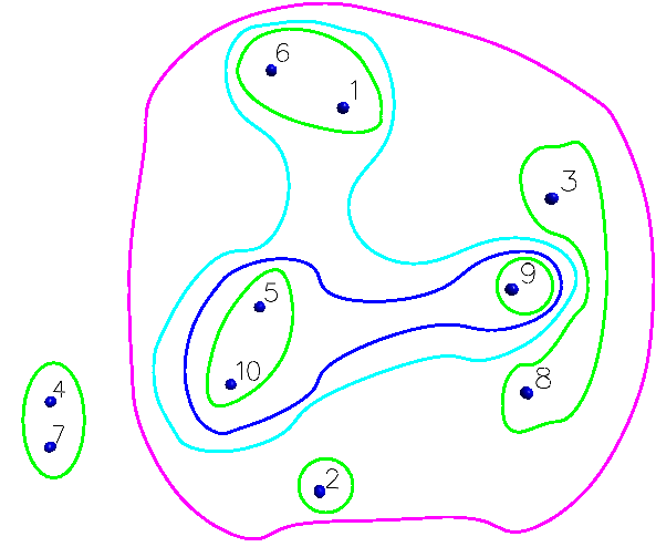
Figure 4: Clustering induced by maximum transfer probability measure for a general spin network shows that clustering differs from what would be expected if we clustered according to physical distance.

V Control of Information Transfer

To overcome intrinsic limitations on quantum state transfer or speed up transfer, one can either try to engineer spin chains or networks with non-uniform couplings or introduce dynamic control to change the network topology. The idea of engineered couplings was originally proposed to achieve perfect state transfer between the end spin in spin chain quantum wires [15]. The analysis above shows that engineering the couplings is not strictly necessary. As the distance between the end spins with regard to the ITC metric defined above is zero for uniform XX and Heisenberg chains, we can achieve arbitrary high fidelities state transfer between the end spins if we wait long enough. Engineering the couplings, however, can speed up certain state transfer tasks such as state transfer between the end spins at the expense of others.

A more flexible alternative to fixed engineered couplings is to apply control. For instance, suppose we would like to transfer an excitation from node $1$ to $4$ for an XX chain of length $N=7$. Node $4$ being the anti-gravity center, the maximum transfer probability without control is low regardless how long we are prepared to wait. If we are able to change the Hamiltonian of the network by applying some control perturbtation so that $H=H_{0}+u(t)H_{1}$ we can change the situation even if the control is restricted to $u(t)=0,1$, and $H_{1}$ is a local perturbation, e.g., of a single spin induced by a magnetic field, e.g., $H_{1}=\sigma_{z}^{(1)}$. Switching the control on/off at times $t_{n}$ induces the evolution

$$U_{u}(t_{n},0)=U_{n-1\!\!\!\mod 2}(t_{n},t_{n-1})\cdots U_{1}(t_{2},t_{1})U_{0}(t_{1},t_{0})$$ (7)

where $U_{0}(t_{k},t_{k-1})=e^{-\imath(t_{k}-t_{k-1})H_{0}}$ and $U_{1}(t_{k},t_{k-1})=e^{-\imath(t_{k}-t_{k-1})(H_{0}+H_{1})}$. By optimizing the control sequence, i.e., in this restricted case the switching times $\{t_{k}\}$, we can change the dynamics to achieve near perfect transfer of an excitation or quantum state to a desired target node. In [16] it was shown that applying a simple bang-bang control sequence to a single spin can significantly speed up quantum state transfer between the ends of a chain, but control also allows us to overcome fundamental limits imposed the maximum ITC, enabling us to achieve near perfect excitation transfer to the anti-gravity center in very short time, as shown in Fig. 5, for example. We can think of the control sequence as implementing an effective Hamiltonian $H_{\rm eff}$ defined by $e^{-iH_{\rm eff}t_{n}}=U_{u}(t_{n},0)$ at time $t_{n}$. This effective Hamiltonian differs from the system Hamiltonian $H_{0}$, as do the transition probabilities. For comparison, we diagonalize the effective Hamiltonian, compute the associated maximum transition probabilities $p_{\rm eff}(i,j)$, and use hierarchical clustering to elucitate the proximity relations between spins under the original and effective Hamiltonian. Fig. 6 shows that the results for a particular control example.

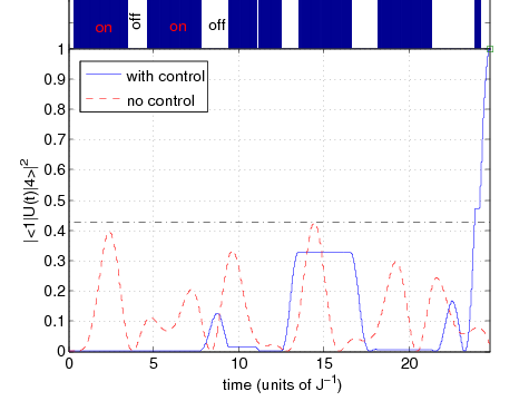
Figure 5: Population of $|4\rangle$ for a uniform chain XX chain of length $N=7$ under free and controlled evolution. Under free evolution (dashed) the population cannot exceed $0.4268$ (dash-dot line) but control can overcome this restriction resulting in near perfect excitation transfer.

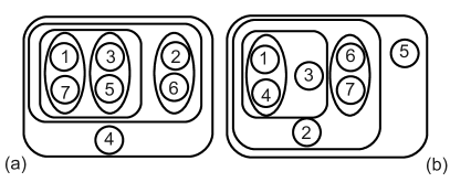
Figure 6: Clustering induced by maximum transfer probability for a uniform chain XX chain of length $N=7$ without control (a) and clustering induced by controlled transition probability (b) for a bang-bang control sequence designed to achieve perfect state transfer from spin $1$ to $4$.

VI Conclusions

Following the recent trend of geometrization of classical communication networks, we have here developed the geometry of spin networks using an Information Transfer Capacity metric. Classical and quantum networks bear the similarity that they are both Gromov hyperbolic, with the difference that classical networks have a Cantor Gromov boundary while spin chains have their Gromov boundary reduced to a point. This probably accounts for yet another discrepancy: classical networks have a gravity center (a congestion point) while quantum networks have an anti-gravity center, a spin difficult to communicate with. The broader implication of this geometrization is that it specifies where control is necessary to overcome such limitations of the physics.

VII Acknowledgments

Edmond Jonckheere acknowledges funding from US National Science Foundation under Grant CNS-NetSE-1017881. Sophie G Schirmer acknowledges funding from EPSRC ARF Grant EP/D07192X/1 and Hitachi. Frank C Langbein acknowledges funding for RIVIC One Wales National Research Centre from WAG.

-A proof of attainability

Theorem 1

If the numbers $\frac{\lambda_{1}}{\pi},\ldots,\frac{\lambda_{N}}{\pi}$ are rationally independent [2, Proposition 1.4.1], then $\forall\epsilon>0$ there exists a $t>0$ large enough such that $p(i,j)-p(i,j,t)<\epsilon$.

Proof:

Set the system of units such that $\hbar=1$. In order to reach the maximum probability exactly, one must find a $t$ such that

$$-\lambda_{k}t=(2m+1)\pi \mbox{ if }\operatorname{Sgn}(v_{ik}v_{jk})=-1$$

$$-\lambda_{k}t=(2m)\pi \mbox{ if }\operatorname{Sgn}(v_{ik}v_{jk})=+1$$

where $v_{ik}=\langle i|v_{k}\rangle$ is the projection of the eigenstate ${\bm{v}_{k}}$ onto the basis state $|i\rangle$, etc, and $v_{ik}^{*}=v_{ik}$ as the eigenstates are real for real-symmetric Hamiltonians. In other words, the state of the $N$-dimensional dynamical system

$$\dot{\tilde{x}}(t)=-\mbox{diag}\left\{\lambda_{1},...,\lambda_{N}\right\},\quad\tilde{x}(0)=0$$

must hit a point whose coordinates are integer multiples of $\pi$, with the correct parity. As the pariety is not affected by the modulo $2\pi$ operation the problem reduces to whether the state of the system

$$\dot{x}(t)=-\mbox{diag}\left\{\lambda_{1},...,\lambda_{N}\right\}\mod 2\pi,\quad x(0)=0$$ (8)

hits a point $x^{*}$ with coordinates $0$ or $\pi$, depending on the signs of the various $v_{ik}v_{jk}$. This dynamical system is the linear flow on the $N$-torus, $\mathbb{T}^{N}$ and by [2, Proposition 1.5.1] it is minimal [2, Definition 1.3.2], that is, the orbit of every point is dense. (Observe that minimality is stronger than topological transitivity [2, Definition 1.3.1]!) Hence we can get arbitrarily close to the point with desired coordinates provided we allow $t$ to be large enough. ∎

To get a quantitative estimate of how close the state $x(t)$ has to be to the target point $x^{*}$ with coordinates $0,\pi$ so that $p(i,j)-p(i,j,t)\leq\epsilon$ note that

$$\sqrt{p(i,j)}= \left|\sum_{k}(\pm 1)v_{ik}v_{jk}\right|$$

$$= \left|\sum_{k}v_{ik}v_{jk}e^{-\imath\lambda_{k}t}+v_{ik}v_{jk}\left(\pm 1-e^{-\imath\lambda_{k}t}\right)\right|$$

$$\leq \sqrt{p(i,j)}+\sum_{k}\left|v_{ij}v_{jk}\left(\pm 1-e^{-\imath\lambda_{k}t}\right)\right|$$

$$\leq \sqrt{p(i,j)}+\sum_{k}\left|\pm 1-e^{-\imath\lambda_{k}t}\right|.$$

Thus we have $\sqrt{p(i,j)}-\sqrt{p(i,j,t)}\leq\sum_{k}\left|\pm 1-e^{-\imath\lambda_{k}t}\right|$. From physical considerations we know that $0\leq p(i,j,t)\leq 1$.

$$p_{\max}-p=\left(\sqrt{p_{\max}}-\sqrt{p}\right)\left(\sqrt{p_{\max}}+\sqrt{p}\right)$$

thus shows that to secure $p_{\max}-p\leq\epsilon$, it suffices to make $\left|\pm 1-e^{-\imath\lambda_{k}t}\right|\leq\frac{\epsilon}{2N}$. If we set $x_{k}(t)=-\lambda_{k}t$ and denote the dynamical target state as $x^{*}_{k}:=0\mbox{ or }\pi$, it suffices that the target state and the actual state are within the specification $|x^{*}_{k}-x_{k}(t)|\leq\sin^{-1}\left(\frac{\epsilon}{2N}\right)$. Since the topology induced by hypercubes is equivalent to the usual topology induced by balls, the latter specification can be achieved by the density of the orbit of $0$.

-B Estimate of time to attain maximum probability

The preceding material only tells us that one can reach arbitrarily closely the maximum probability, but it does not tell us how much time it takes. A conservative estimate can be derived, conservative in the sense that it assumes that the dynamical evolution in $x$ has been discretized as the translation on the torus [2, Sec. 1.4],

$$x(n+1)=x(n)-\mbox{diag}\{\lambda_{1},...,\lambda_{N}\}\quad\bmod 2\pi,\quad x(0)=0$$

The key result is that, under the condition that $\frac{\lambda_{1}}{\pi},...,\frac{\lambda_{N}}{\pi},1$ are rationally independent, the translation on the torus is also minimal [2, Prop. 1.4.1]. In this case, the problem consists in finding $n\in\mathbb{N}$ such that

$$-\lambda_{k}n=(2m+1)\pi \mbox{ if }\operatorname{Sgn}(v_{ik}v_{jk})=-1$$

$$-\lambda_{k}n=(2m)\pi \mbox{ if }\operatorname{Sgn}(v_{ik}v_{ij})=+1$$

is satisfied with arbitrary accuracy, which can be derived from:

Theorem 2 (Nowak[14])

For any $\frac{\lambda_{k}}{\pi}\in\mathbb{R}\setminus\mathbb{Z}$, $k=1,...,N$, there exist infinitely many $((p_{1},...,p_{N}),q)\in\mathbb{Z}^{N}\times\mathbb{N}$ such that

$$\sum_{k=1}^{N}\left|-\frac{\lambda_{k}}{\pi}-\frac{p_{k}}{q}\right|\leq\frac{c_{N}^{-1/N}}{q^{1+1/N}}$$ (9)

where the supremum, $\bar{c}_{N}$, of all $c_{N}$’s satisfying the above is known as $\bar{c}_{1}=\sqrt{5}$, $\bar{c}_{2}=\sqrt{23}/2$, and for larger $N$ estimated as $\bar{c}_{3}\geq 1.7739$, and, for $N\geq 4$, $\bar{c}_{N}\geq(N+1)^{(N+1)/2}N^{-N/2}(\pi/2)^{(N+1)/2}/\Gamma((N+5)/2)$.

We already know by the minimality of the discrete flow, except for the error bound. Therefore, the set of $((p_{1},...,p_{N}),q)\in\mathbb{Z}^{N}\times\mathbb{N}$ of the above theorem and the set of those that satisfy the parity condition have a nonempty intersection. Take a $((p_{1},...,p_{N}),q)$ in this intersection; thus the $p_{k}$ are consistent with the parity condition. Hence

$$\sum_{k=1}^{N}\left|-\frac{\lambda_{k}n}{\pi}-\frac{p_{k}}{q}n\right|<\frac{c_{N}^{-1/N}}{q^{1+1/N}}n$$

Taking $n=q$ yields an $\ell^{1}$ error bound of $c_{N}^{-1/N}/q^{1/N}$ on the $(x/\pi)$-dynamics and furthermore an error bound of $\frac{\pi c_{N}^{-1/N}}{q^{1/N}}=:\epsilon$ on the $x$-dynamics. Thus the time it takes to be within an $\ell^{1}$-ball of “radius” $\epsilon$ around one of the desired points is estimated as $n=q\approx\frac{\pi^{N}c_{N}^{-1}}{\epsilon^{N}}$.

References

- [1] S. Bose Quantum Communication through Spin Chain Dynamics: an Introductory Oview. Contemporary Physics 48:13, 2007.
- [2] A. Katok and B. Hasselblatt. Introduction to the Modern Theory of Dynamical Systems. Cambridge, 1997.
- [3] F. Ariaei, M. Lou, E. Jonckheere, B. Krishnamachari, and M. Zuniga. Curvature of indoor sensor network: clustering coefficient. EURASIP Journal on Wireless Communications and Networking, 2008:20 pages, 2008. Article ID 213185; doi: 10.1155/2008/2131185.
- [4] F. Ariaie and E. Jonckheere. Upper bound on scaled Gromov 4-point delta: Sturm sequence approach. Available upon request.
- [5] I. J. Schoenberg. Remarks to a M. Fréchet’s article. Annals of Mathematics, 36:724–731, 1935.
- [6] L. M. Blumenthal. Theory and Applications of Distance Geometry. Oxford at the Clarendon Press, London, 1953.
- [7] E. Jonckheere, P. Lohsoonthorn, and F. Bonahon. Scaled Gromov hyperbolic graphs. Journal of Graph Theory, 57:157–180, 2008.
- [8] M. Bonk and O. Schramm. Embeddings of Gromov hyperbolic spaces. Geom. Funct. Analysis, 10:266–306, 2000.
- [9] Edmond Jonckheere, Mingji Lou, Francis Bonahon, and Yuliy Baryshnikov. Euclidean versus hyperbolic congestion in idealized versus experimental networks. Internet Mathematics, To appear.
- [10] J. Jost. Nonpositive Curvature: Geometric and Analytic Aspects. Lectures in Mathematics. Birkhauser, Basel-Boston-Berlin, 1997.
- [11] M. Lou, E. Jonckheere, Y. Baryshnikov, F. Bonahon, and B. Krishnamachari. Load balancing by network curvature control. International Journal of Computers, Communications and Control (IJCCC), 6(1):134–149, March 2011.
- [12] Edmond A. Jonckheere, Mingji Lou, Prabir Barooah, and Jo o P. Hespanha. Effective resistance of Gromov-hyperbolic graphs: Application to asymptotic sensor network problems. In IEEE Conference on Decision and Control, pages 1453–1458, New Orleans, LA, December 2007.
- [13] B. I. Mills, F. C. Langbein, A. D. Marshall, and R. R. Martin. Approximate symmetry detection for reverse engineering. In Proc. ACM Symp. Solid Modeling and Applications, pages 241–248, 2001.
- [14] W. G. Nowak. On simultaneous diophantine approximation. Rendiconti del Circolo Matematico di Palermo, XXXIII:456–460, 1984.
- [15] C. Albanese, M. Christandl, N. Datta, A. Ekert, Mirror Inversion of Quantum States in Linear Registers. Phys. Rev. Lett. 93:230502, 2004.
- [16] S. G. Schirmer and P. J. Pemberton-Ross. Fast high-fidelity information transmission through spin-chain quantum wires. Physical review A, 80:030301–1–030301–4, 2009.