Forbidden and intercombination lines of RR Telescopii: wavelength measurements and energy levels

Abstract

Ultraviolet and visible spectra of the symbiotic nova RR Telescopii are used to derive reference wavelengths for many forbidden and intercombination transitions of ions +1 to +6 of elements C, N, O, Ne, Na, Mg, Al, Si, P, S, Cl, Ar, K and Ca. The wavelengths are then used to determine new energy values for the levels within the ions’ ground configurations or first excited configuration. The spectra were measured by the Space Telescope Imaging Spectrograph of the Hubble Space Telescope and the UltraViolet Echelle Spectrograph of the European Southern Observatory in 2000 and 1999, respectively, and cover 1140 to 6915 Å. Particular care was taken to assess the accuracy of the wavelength scale between the two instruments. An investigation of the profiles of the emission lines reveals that the nebula consists of at least two plasma components at different velocities. The components have different densities, and a simple model of the lines’ emissions demonstrates that most of the lines principally arise from the high density component. Only these lines were used for the wavelength study.

1 Introduction

Forbidden lines of ions from low ionization stages having very long decay rates can only be measured in astronomical plasma sources as it is not possible to attain the necessary, very low plasma densities in laboratory plasma sources. For ’coronal’ ions, i.e., those with typically six or more electrons removed, it is possible to measure the forbidden lines in solar spectra taken above the solar limb and measurements obtained from Skylab and SOHO spectra are presented in Doschek et al. (1976b), Doschek et al. (1977), Sandlin et al. (1977) and Feldman & Doschek (2007). For lower ionization stages it is necessary to observe other astronomical sources and, in particular, nebulae. The wavelengths derived by Bowen (1960) are for many forbidden lines still the standard references used in astronomy and the present work seeks to update these values using emission line measurements of the nova RR Telescopii obtained with space-based and ground-based spectrographs. Of particular interest are forbidden lines observed below 3000 Å that were inaccessible at the time of Bowen’s work.

RR Tel has long been a favorite target of spectroscopists on account of its very rich emission line spectrum, and indeed updates to some of the Bowen wavelengths were provided by Thackeray (1977) and Penston et al. (1983) using visible and ultraviolet spectra of RR Tel. The emission lines arise from a nebula that envelopes a late-type giant and hot white dwarf, and the system is classified as a symbiotic nova that went into outburst in 1944. The white dwarf temperature was determined to be around 142,000 K from X-ray observations (Jordan et al., 1994) which is sufficient to produce ionization stages up to +6 in the nebula. Of great value for ultraviolet observations of RR Tel is the low extinction along the line-of-sight towards the system, with $E(B-V)$ values of between 0 and 0.10 determined by different methods (Young et al., 2005a; Selvelli et al., 2007), which ensures strong signals in short wavelength lines. In addition, the interstellar absorption lines are weak in the spectrum and redshifted relative to the system’s radial velocity of $-62$ km s^-1 (Thackeray, 1977).

In the present work new wavelengths for 88 forbidden and intercombination lines belonging to ion species with charge states between +1 and +6 are presented. Careful attention is paid to deriving an accurate rest wavelength scale for both the UV and visible spectra by using lines from low ionization stages, and to deriving accurate error estimates for the wavelengths. The wavelengths are then used in Sect. 7 to derive new energy level values for the ions.

2 Observations

The observations analyzed here were obtained with the Space Telescope Imaging Spectrograph (STIS) on board the Hubble Space Telescope (HST), and with the UVES (Dekker et al., 2000) echelle spectrometer installed at the Kueyen telescope of the Very Large Telescope (VLT). These data have been used previously by Selvelli & Bonifacio (2000), Keenan et al. (2002), Young et al. (2005a), Skopal (2007) and Selvelli et al. (2007) where more details can be found. We summarize the main details here.

The STIS observations were obtained on 2000 October 18 and yielded complete spectra over the wavelength range 1140–7051 Å. The visible spectra in the range 3022–7051 Å were obtained with the STIS CCD and are of low resolution so are not suitable for accurate wavelength measurements. The UV spectra in the range 1140–3120 Å have a high resolution of 30,000–45,000, and were obtained with three exposures. The first used the E140 echelle grating to cover the wavelength range 1140 to 1730 Å, while the following two exposures used the E230M grating to observe the wavelength ranges 1606–2367 and 2274–3120 Å. We will refer to the three STIS exposures as the short, medium and long wavelength (SW, MW and LW) exposures. The data were downloaded from the MAST archive which delivers calibrated 1D spectra. The data analyzed here had been processed with version 2.22 of CALSTIS, the STIS calibration pipeline.

The UVES spectra were obtained in 1999 October and cover two wavelength ranges: 3085–3914 Å and 4730–6915 Å. The spectra were reduced using the MIDAS package by one of the authors (A. Lobel) and have been corrected for the Earth’s motion using a velocity of $-24.6$ km s^-1 (Selvelli & Bonifacio, 2000).

3 Plasma components

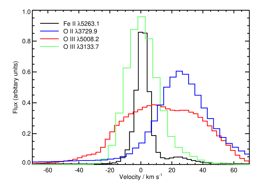
Figure 1: Comparison of line profiles found in the UVES spectrum. The velocity scale has been set to the radial velocity of the system, as determined from Fe ii lines (see text).

The aim of the present work is to derive updated reference wavelengths for forbidden and intercombination transitions of ionized atoms from the RR Tel spectra. This is achieved by first deriving a reference wavelength scale using emission lines with accurately-known wavelengths. A key assumption in the work is that all of the emission lines are emitted from a plasma with the same line-of-sight velocity such that the results are not affected by relative Doppler shifts of different species.

Inspection of certain line profiles (Fig. 1), however, clearly demonstrates that the RR Tel nebula has at least two distinct plasma components with different velocities. This was first noticed by Schild & Schmid (1997) who obtained high resolution line profiles for the density sensitive O iii $\lambda$5007 and $\lambda$4363 forbidden lines. Schild & Schmid (1997) suggested that the O iii emission can be assigned to a high density component at the radial velocity of the star, and a low density component blueshifted relative to this component by 20 km s^-1. The O iii $\lambda$4363 line profile presented by Crawford et al. (1999) also demonstrated ‘rest’ and blueshifted components, although the blueshift was 28 km s^-1 in this case. The authors also presented line profiles from four other emission lines that suggested up to four distinct velocity components in the system. Note that some caution should be attached to the results of these two papers as the Schild & Schmid (1997) work was a brief conference proceedings report with no discussion on how the velocity scale was derived, while Crawford et al. (1999) also did not give details about the derivation of the velocity scale.

The spectra from UVES presented here reveal a different velocity structure than those presented by Schild & Schmid (1997) and Crawford et al. (1999), and which is best illustrated by the line profiles presented in Fig. 1. Four emission line profiles are shown, and the velocity scale has been corrected for the average velocity of the Fe ii forbidden lines (Sect. 5.2). The Fe ii velocity corresponds to the classical radial velocity of the RR Tel nebula (Thackeray, 1950, 1977), and we term this the ‘rest’ component of the nebula. The four profiles belong to three forbidden lines, Fe ii $\lambda$5263.1, O ii 3729.9 and O iii $\lambda$5008.2, and the resonance line O iii 3133.7 which is actually fluoresced through the He ii $\lambda$304 EUV line and so is not optically thick. O ii $\lambda$3729 reveals a broad, nearly symmetric Gaussian that is redshifted by $\approx 20$ km s^-1. A comparison of the strength of this line with the nearby O ii $\lambda$3727.1 (which lies partly in the wing of Ca vi 3726.5, but can be accurately estimated) suggests a density of $<10^{3}$ cm^-3 using the atomic model from the CHIANTI atomic database (Dere et al., 1997, 2009). This is consistent with $\lambda$3729.9 being formed in the low density plasma component found by Schild & Schmid (1997), however the velocity shift is in the opposite direction. We speculate that there may be some time dependence to the velocity of the low density plasma component. Note that Crawford et al. (1999) presented a line profile of O ii $\lambda$4072.2 which showed a two component structure. This is a recombination line and so is formed in the O²⁺ emitting region.

O iii $\lambda$5008.2 shows a complex structure suggesting three plasma components: one at around $+20$ km s^-1 consistent with the O ii line, another at around $+10$ km s^-1, and a further one at around $-30$ to $-40$ km s^-1. It is somewhat similar to the profiles presented by Schild & Schmid (1997) and Crawford et al. (1999) however the main body of the profile here lies near the rest velocity of the system whereas in these two works it was blueshifted by 20–30 km s^-1. O iii $\lambda$3133 shows a strong component at the rest velocity of the system, with an extended wing on the long wavelength side of the profile, which may indicate a small contribution from the low density plasma component. A similar profile is found for a number of strong intercombination lines in the STIS spectrum, including C iii $\lambda$1908.7, O iii $\lambda$1666.2, O iv $\lambda$1401.2 and N iv 1486.5.

Finally we show Fe ii $\lambda$5263.1 which is one of the forbidden lines used to determine the RR Tel radial velocity. The profile actually consists of two components, the stronger is the one used to determine the radial velocity, while the weaker is close in velocity to the O ii $\lambda$3729 line.

The different velocity structure shown by these line profiles presents a fundamental problem: how can an RR Tel emission line be used to determine a rest wavelength for an atomic transition if there is uncertainty over which plasma component the line arises from? Appendix A presents a simple model of the RR Tel nebula represented by low density and high density plasma components. Using the emission models from CHIANTI it is demonstrated that only a small number of emission lines are expected to have significant emission from the low density, red-shifted plasma component (which gives rise to O ii $\lambda$3729.9). The vast majority of the lines studied in the present work predominantly arise from the rest component of the plasma (which gives rise to the strong, narrow component of the Fe ii $\lambda$5263.1 line).

The emission lines shown in Fig. 1 are from low ionization species, yet many of the lines studied in the present work are from higher ionization species. Therefore another uncertainty is whether further plasma components become apparent for higher ionizations that are not revealed in the lower ionization lines. This can be studied by considering two lines of O iv and O v, formed through recombination onto O⁴⁺ (IP=77.4 eV) and O⁵⁺ (IP=113.9 eV). Fig. 2 compares the line profiles of O iv $\lambda$3412.67 and O v $\lambda$2942.51 with two of the Fe ii emission lines used to determine the STIS and UVES rest wavelength scales. The O iv line is the $3p$ ${}^{2}P_{3/2}$ – $3d$ ${}^{2}D_{5/2}$ transition, while O v is $5g$ ${}^{1,3}G$ – $6h$ ${}^{1,3}H$ (an unresolved multiplet). Laboratory wavelengths for these transitions were measured by Bromander (1969) and Bockasten & Johansson (1968), respectively, to accuracies of 0.05 Å (5 km s^-1). The line profiles shown in Fig. 2 show that the line centroids of the two high ionization oxygen lines are in excellent agreement with the Fe ii lines, confirming that the high ionization species are emitted from the rest component of the RR Tel nebula plasma.

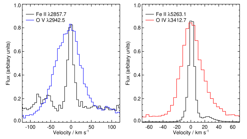
Figure 2: A comparison of high ionization line profiles with profiles for Fe ii wavelength fiducial lines. The left panel shows two profiles from the STIS spectra, the right panel two profiles from the UVES spectra. The velocity scale has been set to the radial velocity of the system as determined from the wavelength fiducial lines (see Sect. 5).

4 Time variability

As the two sets of spectra considered in the present work are separated by a year in time, we briefly discuss the time variability of the RR Tel emission line spectra. RR Tel has had only one known outburst, in 1944, and has evolved rather slowly since then. Thackeray (1977) performed a detailed analysis of the variability of the visible spectrum over the period 1951–1973, and Fig. 8 of this work illustrates the increasing levels of ionization in the nebula for iron over this time. From 1954 to around 1960, the sequence of iron ions from Fe iii to Fe vii progressively peaked and faded, with Fe vii (ionization potential, IP, of 99.1 eV) remaining strong at the end of the observation period. The ion with the highest IP, Ca vii with a value of 108.8 eV, only became apparent in 1968. Although the low ionization species generally declined in strength, they remained present in the spectrum.

RR Tel was regularly observed by IUE, and Zuccolo et al. (1997) presented measurements of emission line fluxes from 1978 to 1993. The level of ionization continued to increase since the work of Thackeray (1977), as best indicated by the emergence of UV lines of Mg vi (IP=141.3 eV) in 1983 which increased in strength by a factor three up to 1993. Comparing with the STIS spectrum of 2000, we find that all of the emission lines in the 1140–1900 Å range have become weaker since 1993, with the lower ionization stages (e.g., Fe ii, O i) by around a factor 10, moderate ionization stages (e.g., O iv, Si iv) by a factor of a few, and the highest ionization stage (Mg vi) by only 40%.

Kotnik-Karuza et al. (2006) have demonstrated that RR Tel has undergone three dust obscuration events, with the most recent in 1996–2000 which coincided with a decline in the visual brightness of RR Tel. Kotnik-Karuza et al. (2009) presented measurements of optical emission lines from 1996 and 2000 and found that all emission lines have declined in flux, with the lower ionization species showing larger falls and the higher ionization species showing smaller falls. This appears to be consistent with the change in ultraviolet emission line fluxes between 1993 and 2000.

No evidence has been presented in the literature for significant short term (timescales of 1 year) changes in the spectrum of RR Tel since the 1944 outburst and, additionally, Zuccolo et al. (1997) found no significant changes in emission line centroids with time for the IUE observations of 1978–1993. It is thus reasonable to assume that the STIS and UVES spectra can be combined to determine rest wavelengths for the system, however the radial velocity discrepancy discussed in Sect. 5.1 may point to a small anomaly between the two observations.

5 Absolute wavelength scale

In order to convert measured wavelengths to energy level separations in the ions, it is necessary to convert them to rest wavelengths. For RR Tel this means correctly establishing the radial velocity of the star (or more precisely the emitting nebula). Since rest wavelengths are accurately known for many low ionization states of elements (typically neutral, singly and doubly-ionized stages) the basic method employed here is to use these ions to establish the radial velocity of the star, which can then be used to place the highly-ionized ion lines on a rest wavelength scale.

The standard radial velocity used for RR Tel is the value $-62.3$ km s^-1 originally derived by Thackeray (1950), although no details were given. Thackeray (1977) cited this earlier result and presented new measurements that were found to be in good agreement with the earlier measurement. Note that Thackeray (1977) suggests the measurements from forbidden Fe ii lines are the most reliable, and these yielded a velocity of $-61.8\pm 0.5$ km s^-1.

Given the high spectral resolution of both the STIS and UVES spectra, it is appropriate to determine afresh the radial velocity using wavelength fiducials in the spectra. Following Thackeray (1977) the most appropriate lines in the optical are the forbidden lines of Fe ii and these will be discussed in Sect. 5.2. The situation is more complicated at the UV wavelengths covered by the STIS spectrum as many of the Fe ii lines are weak resonance transitions that show optical depth effects. Sect. 5.1 discusses the lines chosen here to establish a radial velocity for RR Tel.

5.1 The STIS wavelength scale

This section presents the STIS emission lines that were used as wavelength fiducials to determine the radial velocity of RR Tel and thus allow a wavelength frame to be determined for deriving rest wavelengths for the forbidden lines. Accurate error estimates are important for comparing with previous measurements and so we first give details on how these were determined.

The CALSTIS pipeline assigns 1$\sigma$ errors to the flux measurements at each pixel in the spectra, and these were used in the Gaussian fitting method to determine fitting errors for each line. The second source of error comes from the scatter in the velocities of the wavelength fiducial lines, which we determine as the standard deviation of the lines’ velocities. The three wavelength bands were considered separately and the error values are given later in this section.

A feature of echelle spectrographs is that there is often significant wavelength overlap of adjacent spectral orders, therefore a number of lines are measured twice. All such lines in the three wavelength bands that were isolated and had a good signal were selected, and their centroids determined through Gaussian fitting. The wavelength difference between the two occurrences of a line were determined and converted to a velocity, and then the velocities from all the line pairs in a wavelength band collected and the standard deviation found. For the SW, MW and LW bands the standard deviations were found to be 2.0, 1.5 and 2.1 km s^-1, respectively, and these numbers were treated as the third source of error.

A fourth source of errors was found by considering those ions for which an energy level has two decay paths. E.g., consider a three level ion where level 3 decays to level 2, giving an emission line of wavelength $\lambda_{32}$, and level 2 decays to level 1 giving an emission line of wavelength $\lambda_{21}$. Now suppose level 3 also decays directly to level 1 giving a line at wavelength $\lambda_{31}$. The three wavelengths are related by $\lambda_{31}^{-1}=\lambda_{32}^{-1}+\lambda_{21}^{-1}$, thus by measuring two of the line wavelengths one can predict the position of the third line. Six ions in the combined STIS and UVES spectra allow this check to be performed and the results and consequences on the error analysis are discussed in Sect. 5.3. We find that this error source dominates the others.

The rest wavelength scales for the three STIS channels were determined independently using emission lines from low ionization species for which laboratory wavelengths are accurately known. The criteria for choosing these lines are as follows:

1. the energy levels given in the NIST database must be accurate to 2 decimal places (or better);

2. resonance lines are not used except where optical depth effects are negligible; and

3. the lines are unblended and unaffected by interstellar absorption.

Criterion 1 restricts the selection to low ionization stages (neutral, singly-charged and doubly-charged) since the more highly-charged ions have less accurately known energies (which is in fact the motivation for this work). Criterion 2 follows from the fact that most resonance lines show a significant redshift compared to other lines, and are often asymmetric and/or broadened. For example, the strong resonance lines N v $\lambda$1238 and C iv $\lambda$1548 yield velocities of $-59$ and $-55$ km s^-1, compared to the final radial velocity of $-65$ to $-70$ km s^-1 found below. Considering lines of Fe ii, the resonance lines of UV multiplets 1 and 2 have widths of around 30–40 km s^-1, much larger than those of multiplets excited through radiative pumping such as 391 and 399 which have widths of 15–25 km s^-1. These latter Fe ii lines, although resonance transitions themselves, are not excited from the ground levels of Fe ii and so not subject to photon trapping. They are discussed further in Sect. 5.1.9 below.

The numbers of reference lines for the SW, MW and LW channels are 7, 8 and 35, respectively. The high number for the LW channel reflects the large number of Fe ii lines. The average radial velocities derived for the three channels are $-65.2\pm 1.8$, $-68.3\pm 1.2$ and $-69.7\pm 1.7$ km s^-1. Each emission line measured in the three channels was corrected by the relevant velocity to yield the rest wavelength.

We note that the radial velocity for the SW channel is not consistent with those of the MW and LW channels, and all three velocities are inconsistent with the UVES radial velocity of $-62.6\pm 1.3$ km s^-1 (Sect. 5.2). The latter is close to the radial velocity found by previous authors for RR Tel, suggesting that the STIS absolute velocity scale shows discrepancies of up to 7 km s^-1. It is possible that the cool lines in the RR Tel spectrum have moved by around 5–7 km s^-1 between 1999 and 2000, but this would be surprising given the relatively slow changes previously recorded in the RR Tel spectra. The discrepancy between the radial velocities is not a direct problem for the current work since we are interested in velocities relative to the radial velocity. The only problem would be if the low ionization, reference lines had drifted in velocity relative to the higher ionization lines, but the comparisons presented in Fig. 2 suggest that this is not the case.

The following sections discuss the individual ions and emission lines used as wavelength fiducials, and Table 1 gives the radial velocities from the selected reference lines.

5.1.1 O I

The $2s^{2}2p^{3}(^{4}S)3s$ ${}^{3}S_{1}$ level in O i is believed to be excited in giant stars through radiative pumping of the $2s^{2}2p^{3}(^{4}S)3d$ ${}^{3}D_{J}$ levels by H i Ly$\beta$: the ${}^{3}D$ levels decay to $2s^{2}2p^{3}(^{4}S)3p$ ${}^{3}P_{J}$, which in turn decay to the ${}^{3}S_{1}$ level, strongly enhancing the level’s population (Haisch et al., 1977). ${}^{3}S_{1}$ decays to the three ${}^{3}P_{J}$ levels in the ground configuration, giving rise to lines at 1302.2, 1304.9 and 1306.0 Å. Since $\lambda$1302.2 is a decay to the ground level of O i, interstellar neutral oxygen strongly absorbs the stellar spectrum at this wavelength, but the high radial velocity of the star leaves a portion of the stellar emission line which, however, is not useful for the present study. $\lambda$1304.9 is completely removed from the spectrum by interstellar Si ii $\lambda$1304.370. The remaining line, $\lambda$1306.0, is unaffected by interstellar absorption.

A further decay from ${}^{3}S_{1}$ occurs to the ${}^{1}D_{2}$ level in the ground configuration giving a line at 1641.305 Å, and this is found in the long wavelength wing of the very strong He ii $\lambda$1640.4. The line thus sits on a sloping background and was fit here with a single Gaussian rather than by attempting a double-Gaussian fit to the two lines together. The width of $\lambda$1641.305 is very narrow at 11.4 km s^-1, compared to 41.5 km s^-1 for $\lambda$1306.0. This implies that $\lambda$1306.0 is optically thick, which is confirmed by the flux ratio of 1.6 ($\lambda$1641.3/$\lambda$1306.0) which is much larger than the theoretical branching ratio of $2\times 10^{-5}$. For this reason $\lambda$1306.0 is not included in Table 1.

5.1.2 C III

Four lines are available for C iii with the strongest line, $\lambda$1908.7, showing a clearly asymmetric line profile with an extended long wavelength wing. The wing is likely related to the red-shifted, low density plasma components discussed in Sect. 3. The line profile was fitted with two Gaussians, each forced to have the same width, and the stronger, short wavelength Gaussian was assumed to correspond to the radial velocity of the system and the wavelength is given in Table 1. The weak forbidden line $\lambda$1906.7 is found to be redshifted relative to the expected wavelength by around 20 km s^-1 and Appendix A demonstrates that this is consistent with the line being formed in the redshifted, low density plasma component. It therefore is not useful as a wavelength fiducial here.

The remaining two lines, $\lambda$1247.4 and $\lambda$2297.6, are significantly weaker than $\lambda$1908.7 but have very similar line widths to this line and so appear to be unblended. Both lines are listed in Table 1.

The $2s2p$ ${}^{3}P_{J}$ – $2p^{2}$ ${}^{3}P_{J^{\prime}}$ multiplet is found at around 1175 Å but the spectrum is noisy in this region and ratios of the multiplet’s lines vary significantly from the optically thin case suggesting the lines are optically thick and possibly absorbed by the interstellar medium so they are not used as velocity references.

5.1.3 O III

The intercombination lines at 1660.8 and 1666.2 Å are very strong in RR Tel and show asymmetric profiles similar to C iii $\lambda$1908.7 discussed in the previous section. The centroids were derived in the same manner as the C iii line using two Gaussians of equal width. The O iii lines are found in both the SW and MW spectra but for both they are found to be around 3 km s^-1 blue-shifted relative to the other wavelength reference lines. For this reason they have not been used as reference lines.

The forbidden ${}^{3}P_{1}$–${}^{1}S_{0}$ transition at 2321.7 Å is strong in the RR Tel spectrum and has an asymmetric profile, with the long wavelength wing being significantly stronger than for the intercombination lines. Since the O iii forbidden lines in the visible have unusual profiles (Sect. 3) it was decided not to include the $\lambda$2321.7 line in the present analysis.

Ten Bowen fluorescence lines of O iii are found between 2800 and 3060 Å. The strongest lines, $\lambda$2837 and $\lambda$3048, clearly show asymmetric profiles similar to $\lambda$$\lambda$1660.8, 1666.2. The three lines at 2819.5, 3036.3 and 3060.2 Å were chosen as velocity references as they are each isolated in the spectrum and so unaffected by blending.

5.1.4 Mg II

The strong $\lambda$2796.4, 2803.5 resonance lines are not suitable as wavelength references as they are redshifted relative to other species, suggesting they are affected by P Cygni like absorption on the short wavelength side of their profiles. In addition both lines have strong interstellar absorption features on their long wavelength sides. The much weaker $3p$ ${}^{2}P_{3/2}$ – $3d$ ${}^{2}D_{5/2}$ transition lies between the two strong resonance lines at 2798.82 Å and is suitable as a wavelength reference. A further $3p$–$3d$ transition occurs at 2791.60 Å but is blended, probably with a Fe v transition. $3p$ ${}^{2}P_{3/2}$ – $4s$ ${}^{2}S_{1/2}$ is also found in the STIS spectrum at 2937.37 Å but it is very weak and is not used as a wavelength reference here.

5.1.5 Al II

The intercombination line at 2669.9 Å is unblended and does not show an asymmetric profile. Another Al ii line is the strong resonance transition at 1670.8 Å, however this clearly shows interstellar absorption on the long wavelength side of the profile and so is not suitable as a velocity reference.

5.1.6 Si II

The intercombination lines, $3s^{2}3p$ ${}^{2}P_{J}$ – $3s3p^{2}$ ${}^{4}P_{J^{\prime}}$, are found between 2329 and 2351 Å. The weakest line, $\lambda$2329.24, is too faint to be observed while $\lambda$2344.92 is coincident with Fe ii interstellar absorption and is not seen. The line at 2350.89 Å is close to Si vii $\lambda$2350.73, but this line will be very weak based on the strength of Si vii $\lambda$2147.40 and so we use $\lambda$2350.89 as a reference. The strongest line of the Si ii multiplet is $\lambda$2335.32 however this is notably broader than $\lambda$2350 which is likely due to blends from Si ii $\lambda$2335.12 (part of the same multiplet) and Fe ii $\lambda$2335.18. It is not possible to separate these components and so we do not use $\lambda$2335.32 as a wavelength reference.

5.1.7 Si III

As with other strong resonance lines, Si iii $\lambda$1206.5 is redshifted relative to other lines in the spectrum, and it also shows interstellar absorption on the long wavelength side of the profile. We thus do not use it as a wavelength reference. The intercombination line, $\lambda$1892.0 is actually much stronger than $\lambda$1206.5 and, like other strong intercombination lines in the spectrum, has an asymmetric line profile. The line has been fit with two Gaussians of equal width and the shorter wavelength component is taken to be at the radial velocity of the star. $\lambda$2542.6 is a much weaker line, but is narrow and unblended and we list it in Table 1.

5.1.8 S III

The $3s^{2}3p^{2}$ ${}^{3}P_{1,2}$ – $3s3p^{3}$ ${}^{5}S_{2}$ intercombination lines at 1713.1 and 1728.9 Å are narrow, although fairly weak, and suitable as wavelength references.

5.1.9 Fe II

Fe ii gives rise to more lines than any other species in the RR Tel spectrum and accurate wavelengths are known for many of them. However, many of the Fe ii lines are weak and/or blended which means care has to be taken in selecting lines as wavelength references. In addition it is noticeable that a number of the stronger Fe ii transitions are broad and redshifted relative to the other transitions. Examples include $a~{}^{6}D_{7/2}$–$z~{}^{6}D_{9/2}$ ($\lambda$2626.451), $a~{}^{6}G_{9/2}$–$z~{}^{6}H_{11/2}$ ($\lambda$2459.528) and $a~{}^{6}D_{9/2}$–$z~{}^{6}F_{11/2}$ ($\lambda$2382.765), which have velocities of $-60$ to $-62$ km s^-1 and widths of 30 to 45 km s^-1, compared to $-66$ to $-70$ km s^-1 and 15 to 25 km s^-1 for more typical lines.

There are few Fe ii lines in the STIS SW spectrum and we have used three lines between 1360 and 1414 Å. $\lambda$1360.2 is a narrow, well-observed line which was first identified as being fluoresced by H i Ly$\alpha$ by Johansson & Carpenter (1988), although O v $\lambda$1218.3 may also contribute to the radiative pumping (Hartman & Johansson, 2000). $\lambda$1392.1 and $\lambda$1413.7 are both excited through radiative pumping by He ii $\lambda$1084.9 and were identified by Hartman & Johansson (2000) and Jordan & Harper (1998), respectively.

Only two Fe ii lines in the MW spectrum are used as wavelength fiducials, and both arise from the $z~{}^{4}H_{11/2}$ level which is radiatively pumped by C iv $\lambda$1548.2 (Johansson, 1983) giving rise to 10 lines in all that are very prominent in the RR Tel Fe ii spectrum . Of the ten lines three are anomalously broad, indicating blending, and a fourth ($\lambda$2168.105) shows an anomalous blueshift. The six remaining lines have narrow widths between 20 and 25 km s^-1 and velocity shifts between $-67$ and $-70$ km s^-1 and have been used as reference lines.

The remaining Fe ii lines used for the wavelength calibration are all found in the LW spectrum and arise from four multiplets that are excited through radiative pumping by H i Ly$\alpha$, either directly or by cascading from fluoresced levels. There are four groups of lines in all, three corresponding to UV multiplets 78, 391 and 399, and a fourth corresponding to the unnumbered multiplet $z~{}^{4}P$–$e~{}^{4}D$.

UV multiplet 78 ($a~{}^{4}P$–$z~{}^{4}P$) gives rise to seven lines between 2944 and 3003 Å, which is a region less crowded than other parts of the STIS RR Tel spectrum. One line ($\lambda$2965.489) is a known blend with another Fe ii transition, but the remaining six lines have narrow widths between 20 and 23 km s^-1 and velocities ranging from $-67$ to $-71$ km s^-1, with an average of $-68.9$ km s^-1.

Five lines from UV multiplet 391 ($z~{}^{4}F$–$e~{}^{4}D$) are found in the RR Tel spectrum between 2840 and 2867 Å. Each line is unblended and the line widths range from 13 to 19 km s^-1, and the velocities from $-70$ to $-71$ km s^-1.

UV multiplet 399 ($z~{}^{4}D$–$e~{}^{4}D$) is also emitted from the e ${}^{4}D$ levels, and seven lines are found in the RR Tel spectrum between 2845 and 2886 Å. One line ($\lambda$2885.611) is significantly broader than the others, indicating it is blended. The remaining lines have narrow widths between $-15$ and $-18$ km s^-1 and velocities between $-70$ and $-72$ km s^-1.

Six lines are observed from the unnumbered UV multiplet $z~{}^{4}P$–$e~{}^{4}D$ between 3037 and 3080 Å. Five of these lines have never previously been reported in the RR Tel spectrum, with the remaining line ($\lambda$3079.574) first being reported by Jordan & Harper (1998). All of the lines appear to be unblended, with narrow line widths of between 16 and 25 km s^-1 and velocities between $-67$ and $-73$ km s^-1.

Table 1: Wavelength fiducial lines for RR Tel STIS spectrum.

			$\lambda_{\rm NIST}$	Velocity
Channel	Ion	Transition	(Å)	(km s-1)
SW	O i	$3s^{2}3p^{4}$ ${}^{1}D_{2}$ – $3s3p^{5}$ ${}^{3}S_{1}$	1641.305	$-67.0$
	C iii	$2s2p$ ${}^{1}D_{2}$ – $2p^{2}$ ${}^{1}S_{0}$	1247.383	$-65.4$
	Fe ii	$b~{}^{4}D_{5/2}$ – $(^{3}P)4s4p$ ${}^{4}F_{7/2}$	1360.178	$-67.7$
	Fe ii	$b~{}^{2}H_{11/2}$ – $u~{}^{2}G_{9/2}$	1392.148	$-64.0$
	Fe ii	$a~{}^{4}H_{11/2}$ – $sp~{}x~{}^{4}H_{11/2}$	1413.702	$-62.8$
	S iii	$3s^{2}3p^{2}$ ${}^{3}P_{1}$ – $3s3p^{3}$ ${}^{5}S_{2}$	1713.114	$-63.7$
	S iii	$3s^{2}3p^{2}$ ${}^{3}P_{2}$ – $3s3p^{3}$ ${}^{5}S_{2}$	1728.942	$-65.7$
MW	S iii	$3s^{2}3p^{2}$ ${}^{3}P_{1}$ – $3s3p^{3}$ ${}^{5}S_{2}$	1713.114	$-69.0$
	S iii	$3s^{2}3p^{2}$ ${}^{3}P_{2}$ – $3s3p^{3}$ ${}^{5}S_{2}$	1728.942	$-69.2$
	Si iii	$3s^{2}$ ${}^{1}S_{0}$ – $3s3p$ ${}^{3}P_{1}$	1892.030	$-66.6$
	C iii	$2s^{2}$ ${}^{1}S_{0}$ – $2s2p$ ${}^{3}P_{1}$	1908.734	$-69.1$
	Fe ii	$a~{}^{4}H_{13/2}$ – $y~{}^{4}H_{11/2}$	2211.806	$-70.1$
	Fe ii	$a~{}^{4}H_{11/2}$ – $y~{}^{4}H_{11/2}$	2220.585	$-67.2$
	C iii	$2s2p$ ${}^{1}P_{1}$ – $2p^{2}$ ${}^{1}D_{2}$	2297.587	$-67.6$
	Si ii	$3s^{2}3p$ ${}^{2}P_{3/2}$ – $3s3p^{2}$ ${}^{4}P_{1/2}$	2350.892	$-66.6$
LW	C iii	$2s2p$ ${}^{1}P_{1}$ – $2p^{2}$ ${}^{1}D_{2}$	2297.587	$-69.8$
	Si ii	$3s^{2}3p$ ${}^{2}P_{3/2}$ – $3s3p^{2}$ ${}^{4}P_{1/2}$	2350.892	$-66.7$
	Fe ii	$a~{}^{4}G_{11/2}$ – $y~{}^{4}H_{11/2}$	2436.959	$-68.9$
	Fe ii	$b~{}^{2}H_{11/2}$ – $y~{}^{4}H_{11/2}$	2481.799	$-69.1$
	Fe ii	$b~{}^{2}H_{9/2}$ – $y~{}^{4}H_{11/2}$	2493.096	$-66.6$
	Si iii	$3s3p$ ${}^{1}P_{1}$ – $3p^{2}$ ${}^{1}D_{2}$	2542.581	$-66.6$
	Al ii	$3s^{2}$ ${}^{1}S_{0}$ – $3s3p$ ${}^{3}P_{1}$	2669.948	$-69.7$
	Fe ii	$b~{}^{2}G_{9/2}$ – $y~{}^{4}H_{11/2}$	2772.004	$-68.3$
	Mg ii	$3p$ ${}^{2}P_{3/2}$ – $3d$ ${}^{2}D_{5/2}$	2798.823	$-70.3$
	O iii	$2p3p$ ${}^{3}D_{2}$ – $2p3d$ ${}^{3}P_{2}$	2819.527	$-70.4$
	Fe ii	$z~{}^{4}F_{9/2}$ – $e~{}^{4}D_{7/2}$	2840.348	$-69.6$
	Fe ii	$z~{}^{4}D_{1/2}$ – $e~{}^{4}D_{1/2}$	2845.795	$-70.1$
	Fe ii	$z~{}^{4}D_{3/2}$ – $e~{}^{4}D_{3/2}$	2846.261	$-71.1$
	Fe ii	$z~{}^{4}F_{7/2}$ – $e~{}^{4}D_{5/2}$	2846.433	$-70.1$
	Fe ii	$z~{}^{4}D_{5/2}$ – $e~{}^{4}D_{5/2}$	2848.944	$-70.7$
	Fe ii	$z~{}^{4}F_{5/2}$ – $e~{}^{4}D_{3/2}$	2849.157	$-70.7$
	Fe ii	$z~{}^{4}F_{3/2}$ – $e~{}^{4}D_{1/2}$	2852.561	$-69.4$
	Fe ii	$z~{}^{4}D_{7/2}$ – $e~{}^{4}D_{7/2}$	2857.748	$-70.4$
	Fe ii	$z~{}^{4}D_{1/2}$ – $e~{}^{4}D_{3/2}$	2859.469	$-71.4$
	Fe ii	$z~{}^{4}F_{1/2}$ – $e~{}^{4}D_{1/2}$	2866.301	$-71.4$
	Fe ii	$z~{}^{4}D_{3/2}$ – $e~{}^{4}D_{5/2}$	2870.155	$-70.7$
	Fe ii	$a~{}^{4}P_{1/2}$ – $z~{}^{4}P_{3/2}$	2945.257	$-70.5$
	Fe ii	$a~{}^{4}P_{5/2}$ – $z~{}^{4}P_{3/2}$	2948.516	$-68.6$
	Fe ii	$a~{}^{4}P_{3/2}$ – $z~{}^{4}P_{3/2}$	2965.899	$-69.2$
	Fe ii	$a~{}^{4}P_{5/2}$ – $z~{}^{4}P_{5/2}$	2985.695	$-67.0$
	Fe ii	$a~{}^{4}P_{3/2}$ – $z~{}^{4}P_{1/2}$	2986.416	$-69.0$
	Fe ii	$a~{}^{4}P_{3/2}$ – $z~{}^{4}P_{5/2}$	3003.521	$-69.2$
	O iii	$2p3s$ ${}^{3}P_{1}$ – $2p3p$ ${}^{3}P_{1}$	3036.298	$-69.0$
	Fe ii	$z~{}^{4}P_{5/2}$ – $e~{}^{4}D_{5/2}$	3037.847	$-71.1$
	Fe ii	$z~{}^{4}P_{3/2}$ – $e~{}^{4}D_{3/2}$	3049.878	$-73.1$
	Fe ii	$z~{}^{4}P_{1/2}$ – $e~{}^{4}D_{1/2}$	3056.240	$-70.8$
	O iii	$2p3s$ ${}^{3}P_{2}$ – $2p3p$ ${}^{3}P_{1}$	3060.199	$-74.1$
	Fe ii	$z~{}^{4}P_{1/2}$ – $e~{}^{4}D_{3/2}$	3072.017	$-69.5$
	Fe ii	$z~{}^{4}P_{3/2}$ – $e~{}^{4}D_{5/2}$	3077.329	$-70.0$
	Fe ii	$z~{}^{4}P_{5/2}$ – $e~{}^{4}D_{7/2}$	3079.574	$-67.5$

5.2 The UVES wavelength scale

For the UVES spectra, 23 emission lines of Fe ii were used to derive the radial velocity of the star which was then subtracted to yield the absolute wavelength scale. The emission lines are principally forbidden lines, although the strong allowed multiplet, a ${}^{4}P$–z ${}^{4}D$, was also used. The full list of transitions with measured and rest wavelengths, and derived velocities are shown in Table 5.2. Rest wavelengths have been derived using the Fe ii experimental energies tabulated by Fuhr & Wiese (2006). The average velocity is $-62.6$ km s^-1, with a standard deviation of 1.3 km s^-1. By comparing measured centroids of lines observed in two spectral orders we estimate individual centroid measurements are accurate to approximately $\pm$ 1.5 km s^-1. Combining these two uncertainties with that of the wavelength consistency check discussed in Sect. 5.3 yields the final error estimate for line centroids measured from the UVES spectra. We note that the radial velocity derived from the UVES Fe ii lines is in good agreement with the values of Thackeray (1950) and Thackeray (1977).

Table 2: UVES Fe ii velocities.

$\lambda_{\rm vac}$			Velocity
(Å)	Multiplet	Transition	(km s-1)
3187.659	45	a ${}^{4}P_{3/2}$ – z ${}^{4}D_{3/2}$	$-63.9$
3193.832	45	a ${}^{4}P_{5/2}$ – z ${}^{4}D_{5/2}$	$-64.1$
3194.722	45	a ${}^{4}P_{1/2}$ – z ${}^{4}D_{1/2}$	$-64.2$
3211.371	45	a ${}^{4}P_{1/2}$ – z ${}^{4}D_{3/2}$	$-62.7$
3214.237	45	a ${}^{4}P_{3/2}$ – z ${}^{4}D_{5/2}$	$-63.0$
3228.674	45	a ${}^{4}P_{5/2}$ – z ${}^{4}D_{7/2}$	$-63.2$
4815.880	21	a ${}^{4}F_{9/2}$ – b ${}^{4}F_{9/2}$	$-64.7$
4890.982	5	a ${}^{6}D_{7/2}$ – b ${}^{4}P_{5/2}$	$-64.1$
4906.709	21	a ${}^{4}F_{7/2}$ – b ${}^{4}F_{7/2}$	$-61.8$
5109.365	19	a ${}^{4}F_{5/2}$ – b ${}^{4}P_{1/2}$	$-60.1$
5113.051	20	a ${}^{4}F_{9/2}$ – a ${}^{4}H_{11/2}$	$-61.8$
5165.390	37	a ${}^{4}D_{7/2}$ – a ${}^{2}F_{7/2}$	$-64.7$
5183.391	19	a ${}^{4}F_{3/2}$ – b ${}^{4}P_{1/2}$	$-62.2$
5221.512	20	a ${}^{4}F_{7/2}$ – a ${}^{4}H_{9/2}$	$-62.1$
5263.085	20	a ${}^{4}F_{7/2}$ – a ${}^{4}H_{11/2}$	$-61.6$
5270.341	19	a ${}^{4}F_{5/2}$ – b ${}^{4}P_{3/2}$	$-61.5$
5274.814	19	a ${}^{4}F_{9/2}$ – b ${}^{4}P_{5/2}$	$-61.4$
5298.303	20	a ${}^{4}F_{5/2}$ – a ${}^{4}H_{7/2}$	$-61.2$
5335.129	20	a ${}^{4}F_{5/2}$ – a ${}^{4}H_{9/2}$	$-63.0$
5377.947	20	a ${}^{4}F_{3/2}$ – a ${}^{4}H_{7/2}$	$-62.9$
5434.640	19	a ${}^{4}F_{7/2}$ – b ${}^{4}P_{5/2}$	$-63.0$
5478.764	36	a ${}^{4}D_{3/2}$ – b ${}^{2}P_{1/2}$	$-59.9$
5748.560	36	a ${}^{4}D_{5/2}$ – b ${}^{2}P_{3/2}$	$-63.2$

Table 3: Measured wavelengths.

Transition	$\lambda_{\rm vac}$ (Å)	$\lambda_{\rm air}$ (Å)	$\sigma_{\lambda}$ (Å)	$\lambda_{\rm NIST}$    (Å)	Previous (Å)	Source
Beryllium isoelectronic sequence
N iv
$2s^{2}$ ${}^{1}S_{0}$ – $2s2p$ ${}^{3}P_{1}$	1486.502	1486.502	0.030	1486.496	$1486.48\pm 0.05$	P83
					$1486.51\pm 0.04$	D76
					$1486.52\pm 0.02$	S77
O v
$2s^{2}$ ${}^{1}S_{0}$ – $2s2p$ ${}^{3}P_{2}$	1213.807	1213.807	0.029	1213.809	$1213.90\pm 0.05$	S77
$2s^{2}$ ${}^{1}S_{0}$ – $2s2p$ ${}^{3}P_{1}$	1218.349	1218.349	0.025	1218.344	$1218.35\pm 0.02$	S77
					$1218.35\pm 0.04$	D76
					$1218.37\pm 0.05$	P83
Boron isoelectronic sequence
C ii
${}^{2}P_{1/2}$–${}^{4}P_{3/2}$	2324.272	2323.558	0.047	2324.214	$2323.42\pm 0.05$	P83 (air)
					$2323.52\pm 0.04$	D77 (air)
${}^{2}P_{1/2}$–${}^{4}P_{1/2}$	2325.411	2324.697	0.046	2325.403	$2324.69\pm 0.05$	P83 (air)
					$2324.72\pm 0.04$	D77 (air)
${}^{2}P_{3/2}$–${}^{4}P_{5/2}$	2326.120	2325.406	0.045	2326.113	$2325.38\pm 0.05$	P83 (air)
					$2325.40\pm 0.04$	D77 (air)
${}^{2}P_{3/2}$–${}^{4}P_{3/2}$	2327.669	2326.954	0.047	2327.645	$2326.92\pm 0.05$	P83 (air)
					$2326.98\pm 0.04$	D77 (air)
${}^{2}P_{3/2}$–${}^{4}P_{1/2}$	2328.871	2328.156	0.046	2328.838	$2328.08\pm 0.05$	P83 (air)
					$2328.14\pm 0.04$	D77 (air)
N iii
${}^{2}P_{1/2}$–${}^{4}P_{3/2}$	1746.816	1746.816	0.037	1746.823	$1746.81\pm 0.02$	S77
					$1746.82\pm 0.04$	D76
					$1746.77\pm 0.05$	P83
${}^{2}P_{1/2}$–${}^{4}P_{1/2}$	1748.637	1748.637	0.035	1748.646	$1748.63\pm 0.02$	S77
					$1748.63\pm 0.04$	D76
					$1748.63\pm 0.05$	P83
${}^{2}P_{3/2}$–${}^{4}P_{5/2}$	1749.663	1749.663	0.034	1749.674	$1749.67\pm 0.01$	S77
					$1749.67\pm 0.04$	D76
					$1749.64\pm 0.05$	P83
${}^{2}P_{3/2}$–${}^{4}P_{3/2}$	1752.139	1752.139	0.035	1752.160	$1752.14\pm 0.01$	S77
					$1752.12\pm 0.04$	D76
					$1752.11\pm 0.05$	P83
${}^{2}P_{3/2}$–${}^{4}P_{1/2}$	1753.974	1753.974	0.035	1753.995	$1753.98\pm 0.01$	S77
					$1753.98\pm 0.04$	D76
					$1753.96\pm 0.05$	P83
O iv
${}^{2}P_{1/2}$–${}^{4}P_{3/2}$	1397.199	1397.199	0.029	1397.232	$1397.20\pm 0.04$	D76
					$1397.22\pm 0.02$	S77
					$1397.18\pm 0.05$	P83
					$1397.219\pm 0.075$	H99
					$1397.166\pm 0.004$	K02
${}^{2}P_{1/2}$–${}^{4}P_{1/2}$	1399.766	1399.766	0.029	1399.780	$1399.77\pm 0.04$	D76
					$1399.78\pm 0.01$	S77
					$1399.75\pm 0.05$	P83
					$1399.785\pm 0.075$	H99
					$1399.731\pm 0.004$	K02
${}^{2}P_{3/2}$–${}^{4}P_{5/2}$	1401.157	1401.157	0.029	1401.157	$1401.16\pm 0.04$	D76
					$1401.17\pm 0.01$	S77
					$1401.14\pm 0.05$	P83
					$1401.168\pm 0.075$	H99
					$1401.115\pm 0.004$	K02
${}^{2}P_{3/2}$–${}^{4}P_{3/2}$	1404.783	1404.783	0.029	1404.806	$1404.79\pm 0.04$	D76
					$1404.80\pm 0.02$	S77
					$1404.77\pm 0.05$	P83
					$1404.797\pm 0.075$	H99
					$1404.740\pm 0.004$	K02
${}^{2}P_{3/2}$–${}^{4}P_{1/2}$	1407.372	1407.372	0.029	1407.382	$1407.38\pm 0.04$	D76
					$1407.39\pm 0.02$	S77
					$1407.36\pm 0.05$	P83
					$1407.387\pm 0.075$	H99
					$1407.333\pm 0.004$	K02
Carbon isoelectronic sequence
N ii
${}^{1}D_{2}$–${}^{1}S_{0}$	5756.205	5754.607	0.116	5756.191	$5754.57\pm 0.04$	B60 (air)
${}^{3}P_{1}$–${}^{1}S_{0}$	3063.791	3062.900	0.129	3063.716	$3062.82\pm 0.02$	B60 (air)
${}^{3}P_{1}$–${}^{5}S_{2}$	2139.683	2139.009	0.045	2139.683	$2138.88\pm 0.05$	P83 (air)
Ne v
${}^{3}P_{1}$–${}^{1}D_{2}$	3346.820	3345.858	0.065	3346.783	$3345.83\pm 0.02$	B60 (air)
${}^{3}P_{2}$–${}^{1}D_{2}$	3426.905	3425.923	0.067	3426.864	$3425.87\pm 0.02$	B60 (air)
${}^{3}P_{1}$–${}^{1}S_{0}$	1574.671	1574.671	0.032	1574.700	$1575.2\pm 1.0$	B60
					$1574.68\pm 0.05$	P83
${}^{3}P_{2}$–${}^{1}S_{0}$	1592.187	1592.187	0.045	1592.206	$1592.7\pm 1.0$	B60
${}^{1}D_{2}$–${}^{1}S_{0}$	2973.968	2973.101	0.061	2974.002	$2974.8\pm 3.0$	B60 (air)
					$2974.00\pm 0.05$	P83 (vac)
${}^{3}P_{2}$–${}^{5}S_{2}$	1145.591	1145.591	0.025	1145.606	$1145.61\pm 0.02$	S77
					$1145.62\pm 0.02$	Y05
Na vi
${}^{3}P_{1}$–${}^{1}D_{2}$	2872.650	2871.808	0.060	2873.563	$2871.1\pm 3.0$	B60 (air)
${}^{3}P_{2}$–${}^{1}D_{2}$	2971.785	2970.918	0.061	2972.740	$2970.0\pm 3.0$	B60 (air)
${}^{1}D_{2}$–${}^{1}S_{0}$	2569.588	2568.818	0.097	2569.637	$2568.9\pm 3.0$	B60 (air)
${}^{3}P_{1}$–${}^{1}S_{0}$	1356.321	1356.321	0.039	1356.558	$1356.2\pm 1.0$	B60
Nitrogen isoelectronic sequence
O ii
${}^{4}S_{3/2}$–${}^{2}P_{3/2}$	2471.200	2470.453	0.051	2471.088	$2470.30\pm 0.02$	B60 (air)
Ne iv
${}^{4}S_{3/2}$–${}^{2}P_{3/2}$	1601.502	1601.502	0.033	1601.504	$1602.0\pm 3.0$	B60
					$1601.47\pm 0.05$	P83
${}^{4}S_{3/2}$–${}^{2}P_{1/2}$	1601.698	1601.698	0.034	1601.676	$1602.1\pm 3.0$	B60
${}^{4}S_{3/2}$–${}^{2}D_{3/2}$	2422.617	2421.881	0.050	2422.510	$2422.8\pm 3.0$	B60 (air)
					$2422.43\pm 0.05$	P83 (vac)
					$2421.825\pm 0.011$	J98 (air)
${}^{4}S_{3/2}$–${}^{2}D_{5/2}$	2425.212	2424.475	0.054	2425.148	$2425.4\pm 3.0$	B60 (air)
					$2424.97\pm 0.05$	P83 (vac)
					$2424.403\pm 0.013$	J98 (air)
Na v
${}^{4}S_{3/2}$–${}^{2}D_{5/2}$	2069.919	2069.258	0.062	2069.108	$\cdots$	$\cdots$
${}^{4}S_{3/2}$–${}^{2}P_{3/2}$	1365.388	1365.388	0.028	1365.095	$\cdots$	$\cdots$
${}^{4}S_{3/2}$–${}^{2}P_{1/2}$	1366.081	1366.081	0.029	1365.784	$\cdots$	$\cdots$
Mg vi
${}^{2}D_{3/2}$–${}^{2}P_{1/2}$	3503.182	3502.181	0.068	3502.971	$3503.0\pm 3.0$	B60 (air)
${}^{2}D_{3/2}$–${}^{2}P_{3/2}$	3489.892	3488.893	0.068	3489.720	$3488.1\pm 3.0$	B60 (air)
${}^{2}D_{5/2}$–${}^{2}P_{3/2}$	3488.100	3487.102	0.068	3487.675	$3485.5\pm 3.0$	B60 (air)
${}^{4}S_{3/2}$–${}^{2}P_{3/2}$	1190.040	1190.040	0.024	1190.074	$1190.07\pm 0.01$	S77
					$1190.09\pm 0.03$	C04
${}^{4}S_{3/2}$–${}^{2}P_{1/2}$	1191.588	1191.588	0.024	1191.611	$1191.62\pm 0.02$	S77
					$1191.64\pm 0.03$	C04
${}^{4}S_{3/2}$–${}^{2}D_{3/2}$	1805.882	1805.882	0.035	1805.941	$1805.94\pm 0.03$	S77
Oxygen isoelectronic sequence
Ne iii
${}^{3}P_{1}$–${}^{1}S_{0}$	1814.645	1814.645	0.037	1814.559	$1814.65\pm 0.01$	B60
${}^{3}P_{2}$–${}^{1}D_{2}$	3869.849	3868.752	0.078	3869.861	$3868.76\pm 0.02$	B60 (air)
${}^{1}D_{2}$–${}^{1}S_{0}$	3343.414	3342.453	0.067	3343.142	$3342.5\pm 0.3$	B60 (air)
Na iv
${}^{3}P_{2}$–${}^{1}D_{2}$	3242.660	3241.725	0.063	3242.563	$3241.68\pm 0.10$	B60 (air)
${}^{3}P_{1}$–${}^{1}D_{2}$	3363.260	3362.294	0.068	3363.210	$3362.20\pm 0.10$	B60 (air)
Mg v
${}^{3}P_{1}$–${}^{1}S_{0}$	1324.435	1324.435	0.027	1324.575	$1324.4\pm 1.0$	B60
					$1324.44\pm 0.01$	S77
					$1324.40\pm 0.05$	P83
${}^{1}D_{2}$–${}^{1}S_{0}$	2417.628	2416.893	0.052	2418.204	$2416.8\pm 3.0$	B60 (air)
${}^{3}P_{2}$–${}^{1}D_{2}$	2783.644	2782.823	0.057	2783.499	$2783.1\pm 3.0$	B60 (air)
					$2783.66\pm 0.05$	P83 (vac)
${}^{3}P_{1}$–${}^{1}D_{2}$	2928.991	2928.135	0.060	2928.867	$2928.3\pm 3.0$	B60 (air)
					$2928.99\pm 0.05$	P83 (vac)
Al vi
${}^{3}P_{2}$–${}^{1}D_{2}$	2430.248	2429.511	0.050	2429.130	$2430.0\pm 10.0$	B60 (air)
					2429.499	J98 (air)
${}^{3}P_{1}$–${}^{1}D_{2}$	2603.123	2602.345	0.056	2601.795	$2603.0\pm 10.0$	B60 (air)
Magnesium isoelectronic sequence
P iv
$3s^{2}$ ${}^{1}S_{0}$ – $3s3p$ ${}^{3}P_{1}$	1467.434	1467.434	0.031	1467.427	$1467.44\pm 0.03$	S77
					$1467.41\pm 0.05$	P83
S v
$3s^{2}$ ${}^{1}S_{0}$ – $3s3p$ ${}^{3}P_{1}$	1199.162	1199.162	0.025	1199.134	$1199.18\pm 0.01$	S77
					$1199.14\pm 0.05$	P83
Aluminium isoelectronic sequence
S iv
${}^{2}P_{1/2}$–${}^{4}P_{3/2}$	1398.065	1398.065	0.041	1398.040	$1397.98\pm 0.05$	P83
					$1398.044\pm 0.004$	K02
${}^{2}P_{3/2}$–${}^{4}P_{5/2}$	1406.043	1406.043	0.029	1406.016	$1406.03\pm 0.05$	P83
					$1406.06\pm 0.01$	S77
					$1406.052\pm 0.075$	H99
					$1406.004\pm 0.004$	K02
${}^{2}P_{3/2}$–${}^{4}P_{3/2}$	1416.912	1416.912	0.029	1416.887	$1416.91\pm 0.05$	P83
					$1416.93\pm 0.01$	S77
					$1416.925\pm 0.075$	H99
					$1416.872\pm 0.004$	K02
${}^{2}P_{3/2}$–${}^{4}P_{1/2}$	1423.857	1423.857	0.030	1423.839	$1423.89\pm 0.01$	S77
					$1423.860\pm 0.075$	H99
					$1423.790\pm 0.004$	K02
Silicon isoelectronic sequence
Cl iv
${}^{3}P_{1}$–${}^{1}S_{0}$	3119.549	3118.645	0.063	3119.560	$3118.66\pm 0.04$	B60 (air)
${}^{1}D_{2}$–${}^{1}S_{0}$	5324.697	5323.214	0.107	5324.757	$5323.29\pm 0.10$	B60 (air)
Ar v
${}^{3}P_{1}$–${}^{1}D_{2}$	6436.946	6435.165	0.130	6437.629	$6435.10\pm 0.10$	B60 (air)
					6435.10	T77 (air)
${}^{3}P_{1}$–${}^{1}S_{0}$	2691.848	2691.049	0.056	2692.024	$2691.09\pm 0.04$	B60 (air)
					$2691.74\pm 0.05$	P83 (vac)
K vi
${}^{3}P_{1}$–${}^{1}D_{2}$	5603.816	5602.259	0.113	5603.999	$5603.2\pm 3.0$	B60 (air)
${}^{3}P_{2}$–${}^{1}D_{2}$	6230.117	6228.391	0.122	6230.297	$6229.2\pm 3.0$	B60 (air)
${}^{3}P_{1}$–${}^{1}S_{0}$	2368.265	2367.541	0.126	2368.243	$2366.8\pm 3.0$	B60 (air)
Ca vii
${}^{3}P_{1}$–${}^{1}D_{2}$	4940.649	4939.270	0.096	4940.931	$4939.0\pm 10.0$	B60 (air)
					$4939.48\pm 0.20$	T74 (air)
${}^{3}P_{2}$–${}^{1}D_{2}$	5620.140	5618.579	0.110	5620.314	$5616.0\pm 10.0$	B60 (air)
					$5618.58\pm 0.20$	T74 (air)
${}^{3}P_{1}$–${}^{1}S_{0}$	2111.488	2110.819	0.041	2111.643	$\cdots$	$\cdots$
Phosphorus isoelectronic sequence
Ar iv
${}^{4}S_{3/2}$–${}^{2}P_{3/2}$	2854.583	2853.744	0.059	2854.484	$2853.64\pm 0.04$	B60 (air)
					$2853.67\pm 0.05$	P83 (air)
${}^{4}S_{3/2}$–${}^{2}P_{1/2}$	2869.087	2868.245	0.059	2868.988	$2868.16\pm 0.10$	B60 (air)
					$2868.21\pm 0.05$	P83 (air)
K v
${}^{4}S_{3/2}$–${}^{2}P_{3/2}$	2494.968	2494.215	0.065	2494.998	$2494.5\pm 1.0$	B60 (air)
${}^{4}S_{3/2}$–${}^{2}P_{1/2}$	2515.351	2514.594	0.141	2515.211	$2514.5\pm 1.0$	B60 (air)
${}^{2}D_{3/2}$–${}^{2}P_{3/2}$	6223.679	6221.956	0.125	6223.666	$6223.0\pm 10.0$	B60 (air)
Ca vi
${}^{4}S_{3/2}$–${}^{2}P_{3/2}$	2215.177	2214.486	0.057	2215.198	$2215.0\pm 1.0$	B60 (air)
					$2215.15\pm 0.05$	P83 (vac)
${}^{4}S_{3/2}$–${}^{2}P_{1/2}$	2242.704	2242.008	0.044	2242.821	$2242.6\pm 1.0$	B60 (air)
					$2242.69\pm 0.05$	P83 (vac)
${}^{4}S_{3/2}$–${}^{2}D_{3/2}$	3726.359	3725.300	0.075	3726.463	$3727.1\pm 3.0$	B60 (air)
${}^{2}D_{3/2}$–${}^{2}P_{1/2}$	5632.941	5631.376	0.110	5633.295	$5631.0\pm 10.0$	B60 (air)
${}^{2}D_{3/2}$–${}^{2}P_{3/2}$	5462.193	5460.674	0.107	5462.213	$5460.0\pm 10.0$	B60 (air)
					5460.7	T77 (air)
${}^{2}D_{5/2}$–${}^{2}P_{3/2}$	5587.766	5586.213	0.109	5587.810	$5587.0\pm 10.0$	B60 (air)
					5586.2	T77 (air)
Sulphur isoelectronic sequence
Ar iii
${}^{3}P_{1}$–${}^{1}S_{0}$	3110.065	3109.163	0.072	3110.077	$3109.16\pm 0.04$	B60 (air)
					3109.04	T77 (air)
					$3109.01\pm 0.05$	P83 (air)
${}^{1}D_{2}$–${}^{1}S_{0}$	5193.141	5191.694	0.105	5193.262	$5191.82\pm 0.10$	B60 (air)
					5191.65	T77 (air)
K iv
${}^{3}P_{2}$–${}^{1}D_{2}$	6103.525	6101.834	0.123	6103.479	$6101.83\pm 0.10$	B60 (air)
					6101.76	T77 (air)
Ca v
${}^{3}P_{1}$–${}^{1}S_{0}$	2413.600	2412.866	0.050	2413.605	$2412.4\pm 1.0$	B60 (air)
					$2413.57\pm 0.05$	P83 (vac)
${}^{3}P_{2}$–${}^{1}D_{2}$	5310.792	5309.313	0.104	5310.590	$5309.18\pm 0.10$	B60 (air)
					5309.26	T77 (air)

5.3 Consistency checks

For some of the ions considered in the present work, levels can decay by multiple routes to the ground term of the ion and so if all lines in the decay routes can be measured they will serve as a check on the wavelength scales employed for the STIS and UVES spectra. One example is the ${}^{1}S_{0}$ level in carbon, oxygen, silicon and sulphur-like ions which can decay directly to ${}^{3}P_{1}$, or to ${}^{3}P_{1}$ via the ${}^{1}D_{2}$ level. For nitrogen and phosphorus-like ions the ${}^{2}P_{1/2,3/2}$ levels can decay directly to the ground ${}^{4}S_{3/2}$ level, or via the ${}^{2}D_{3/2,5/2}$ levels.

There are six ions for which these consistency checks can be performed in the present work: Ne v, Na vi, Mg vi, Ne iii, Mg v and Ca vi. Three ions, Ne v, Mg vi and Ca vi, have two distinct levels with multiple decay routes, while the remaining three ions have a single level with multiple decay routes, thus in total there are nine distinct consistency checks on the combined STIS–UVES wavelength scale. For each of the nine cases, the decay routes are a direct decay to the ground term and an indirect route via an intermediate level. The checks consisted of measuring the wavelengths of the transitions of the indirect route and using these to predict a wavelength for the direct route. Expressing the difference (predicted $-$ observed) in wavelengths as a velocity we find the average value to be $+2.6$ km s^-1 with a standard deviation of $3.6$ km s^-1, thus there is no systematic difference between short and long wavelength measurements.

The worst agreement between observed and predicted wavelengths is for Mg vi, and it is significantly outside of the combined 1$\sigma$ errors of other sources of error discussed in Sects. 5.1 and 5.2. Agreement between the observed and predicted wavelengths is an absolute requirement necessary for the integrity of the present work. For this reason we introduce an additional error, expressed as a velocity, that forces the Mg vi wavelengths to agree with each other within the 1$\sigma$ errors of the wavelengths. This velocity error is found to be 5.5 km s^-1, and is added in quadrature to the other sources of error discussed earlier. To illustrate the magnitude of the velocity error we show in Fig. 3 the Mg vi $\lambda$1805.9 line profile with the measured line centroid indicated together with the centroid position derived from combining the wavelengths of the two lines from the alternative decay route.

We believe that this additional error source is not due to the instruments, but instead is due to the velocity and density structure of the nebula and the different sensitivities of emission lines to density. For example, if an ion’s emission lines arise from two plasma components at $\pm 10$ km s^-1 and these components have different densities, then a pair of emission lines that are density sensitive will display different line profiles that may lead to different centroid positions for the lines. Since the resolution and sensitivity, particularly of the STIS spectra, are not high enough to clearly resolve detailed structure in the line profiles then this velocity structure may be smoothed over, and only revealed through anomalous centroids for the lines.

Figure 3: Line profile of the Mg vi $\lambda$1805.9+$\lambda$1806.3 self-blend from the STIS spectrum with a two Gaussian fit over-plotted. The solid vertical line indicates the centroid of the fitted Gaussian for $\lambda$1805.9 and the dashed vertical line indicates the centroid position required to satisfy the consistency check discussed in Sect. 5.3.

6 Wavelengths and energy levels

The following sections give details on all the forbidden lines measured for the present work. Also included for some ions are intercombination lines. Generally in laboratory or astronomy literature wavelengths above 2000 Å are given as air wavelengths whereas those below 2000 Å are given as vacuum wavelengths. For the present work we will only use vacuum wavelengths unless otherwise stated. For conversions between air and vacuum wavelengths we use the IDL routines VACTOAIR and AIRTOVAC that are distributed through the Astronomy IDL library and use the formula given by Morton (1991).

Table 3 presents the wavelengths measured in the present work given in both vacuum and air forms. 1$\sigma$ errors on the measurements, calculated as described in Sect. 5 are also given. The NIST database gives energy values for all ions, and the wavelengths derived from these values using version 3 of the online database (Ralchenko et al., 2008) are presented. Some previous wavelength measurements from astrophysical sources are also presented. Thackeray (1974) and Thackeray (1977) give optical wavelengths derived from RR Tel; Penston et al. (1983) give ultraviolet wavelengths measured from IUE spectra of RR Tel; and Jordan & Harper (1998) presented wavelengths for some lines from HST/GHRS RR Tel spectra. Many of the intercombination lines and some of the higher ionization forbidden lines have been measured in solar spectra, and we include values from Doschek et al. (1976b), Doschek et al. (1977), Sandlin et al. (1977) and Curdt et al. (2004). Each of these spectral atlases was obtained above the solar limb where the plasma can be reasonably considered to be at rest. Emission lines observed on the solar disk are well known to show systematic velocity shifts (Doschek et al., 1976a; Peter & Judge, 1999) and so a spectral atlas such as that of Curdt et al. (2001) is not useful for determining rest wavelengths.

In some parts of the text we refer to the atomic models from the CHIANTI database. CHIANTI gives atomic data for modeling the emission processes of forbidden lines which can be useful for determining the detectability of a line if another line from the ion is known.

6.1 Beryllium isoelectronic sequence

For the present work we consider only the intercombination line $2s^{2}$ ${}^{1}S_{0}$ – $2s2p$ ${}^{3}P_{1}$ and the forbidden line $2s^{2}$ ${}^{1}S_{0}$ – $2s2p$ ${}^{3}P_{2}$. Other lines from the Be-like ions are found in the spectra but these are either resonance lines or recombination lines.

6.1.1 N IV

The intercombination line, $\lambda$1486.5, is strong and lies at the edge of two spectral orders in the SW spectrum. The line has an asymmetric line profile with an extended long wavelength wing and has been fit with two Gaussians forced to have the same width. The stronger, short wavelength component is assumed to be at the rest wavelength of the system and the average wavelength from the two spectral orders was used to derive the wavelength given in Table 3. The wavelength is in good agreement with the NIST wavelength, the previous RR Tel measurement of Penston et al. (1983), and the solar measurements of Doschek et al. (1976b) and Sandlin et al. (1977).

The nearby forbidden line, $\lambda$1483.3, is measured but shows a significant redshift relative to the NIST wavelength: the measured wavelength is $1483.385\pm 0.031$ Å compared to the NIST value of 1483.321 Å, equating to a velocity shift of 13 km s^-1. This is consistent with the corresponding forbidden line of C iii (Sect. 5.1.2) and suggests that it too arises from the redshifted plasma component.

6.1.2 O V

The forbidden and intercombination lines lie either side of the very broad interstellar absorption line of H i Ly$\alpha$ at 1213.8 and 1218.3 Å, respectively. The forbidden line was not reported by Penston et al. (1983) from IUE spectra of RR Tel, but is clearly seen in the STIS spectrum. It lies on the sloping wing of the Ly$\alpha$ absorption feature and thus the long wavelength wing will be more absorbed than the short wavelength wing which may create a false blueshift for the line profile. Due to the higher ionization potential of O v we do not expect the forbidden line to be emitted from the low density plasma component as was found for C iii and N iv. The measured centroid lies blueward of the only previous measurement of the $\lambda$1213.8 line (Sandlin et al., 1977), but the wavelength is in excellent agreement with the NIST wavelength.

As with other intercombination lines, $\lambda$1218.3 shows an asymmetric profile with an extended long wavelength wing. The effect is more pronounced in this case, however because of the Ly$\alpha$ absorption on the short wavelength side of the profile. The line has been fit with two Gaussians forced to have equal width and with the short wavelength side of the profile partly masked off to prevent the Ly$\alpha$ absorption distorting the fit. The strongest of the fitted Gaussians is taken to correspond to the rest component of the system and yields the wavelength given in Table 3 which is in good agreement with the previous measurements of Doschek et al. (1976b), Sandlin et al. (1977) and Penston et al. (1983).

6.2 Boron isoelectronic sequence

The intercombination transitions, $2s^{2}2p$ ${}^{2}P_{J}$ – $2s2p^{2}$ ${}^{4}P_{J^{\prime}}$, of the boron sequence are found in the STIS spectrum for C ii, N iii and O iv. The F v lines are expected around 1167 Å but can not be identified.

6.2.1 C II

All five of the C ii intercombination lines are found in the RR Tel spectrum. The four strongest lines all show asymmetric profiles with enhanced long wavelength wings, similar to other intercombination lines in the spectrum, and they were fit with two Gaussians forced to have the same width. The wavelength of the stronger, short wavelength component was used to generate the rest wavelengths in Table 3. For the weakest transition, ${}^{2}P_{1/2}$ – ${}^{4}P_{1/2}$, the asymmetry is not pronounced due to the lower signal-to-noise and a single Gaussian fit was used. The 3/2–3/2 transition at 2327.6 Å has a much more extended long wavelength wing than the other lines which is likely due to the Fe ii a ${}^{6}D_{5/2}$–z ${}^{6}P_{3/2}$ transition at 2328.111 Å. This part of the profile was thus not included in the two Gaussian fit to the C ii line.

The C ii intercombination lines have been previously measured in off-limb solar spectra by Doschek et al. (1977), and in the IUE spectrum of RR Tel by Penston et al. (1983) and the comparison in Table 3 shows good agreement except for the $\lambda$2324.3 and $\lambda$2328.9 lines, where the Penston et al. (1983) wavelengths are significantly shorter than the current wavelengths. (They are also significantly shorter than the Doschek & Feldman 1977 wavelengths.)

One discrepancy that is present for all three sets of measurements comes from deriving the ground ${}^{2}P_{J}$ level splitting by using the two pairs of transitions ${}^{2}P_{1/2,3/2}$–${}^{4}P_{1/2}$ and ${}^{2}P_{1/2,3/2}$–${}^{4}P_{3/2}$. For the current wavelength measurements the latter transition pair yields a splitting of $62.79\pm 0.16$ cm^-1, while the former yields $63.89\pm 0.10$ cm^-1, neither of which is consistent with the very accurate value of 63.39 cm^-1 from Cooksy et al. (1986). This may reflect short scale inhomogeneities in the STIS wavelength or suggest that the wavelengths are affected by the non-Gaussian shapes of the line profiles.

6.2.2 N III

The five intercombination lines are found within 8 Å of each other and all have very similar line widths of around 30 km s^-1, suggesting they are unblended. The two strongest transitions, $\lambda$1749.7 and $\lambda$1752.1, clearly show asymmetric profiles similar to other intercombination lines in the spectrum and have been fit with two Gaussians forced to have the same width. The stronger, shorter wavelength Gaussians are used to derive the rest wavelengths in Table 3. Single Gaussian fits were used for the remaining transitions. The measured wavelengths are in excellent agreement with the solar measurements of Doschek et al. (1976b) and Sandlin et al. (1977). The agreement with the wavelengths of Penston et al. (1983) from IUE spectra of RR Tel are slightly less good, but consistent within the uncertainties.

6.2.3 O IV

The O iv intercombination lines are very strong in RR Tel and have been studied in some detail by previous authors (Harper et al., 1999; Keenan et al., 2002). As with other strong intercombination lines such as C iii $\lambda$1908.7, O iii $\lambda$$\lambda$1660.8, 1666.2 and Si iii $\lambda$1892.0 the O iv lines have asymmetric profiles with the long wavelength wings of the lines being more extended than the short wavelength wings. They have been fit with two Gaussians forced to have the same width, with the stronger component being taken as that of the rest component of the nebula.

Three previous measurements of the lines’ wavelengths have been made from RR Tel spectra by Penston et al. (1983), Harper et al. (1999) and Keenan et al. (2002) from IUE, HST/GHRS and HST/STIS spectra, respectively, the latter work using the same spectra as used here. In addition the lines have also been measured from solar spectra by Doschek et al. (1976b) and Sandlin et al. (1977). Comparing the results in Table 3 it is clear that the Keenan et al. (2002) wavelengths are blueshifted relative to the other results by around 0.02–0.06 Å. We believe this is because the authors used the nearby Si iv resonance lines to determine a rest wavelength scale. We find that these lines, like other resonance lines in the spectrum, are redshifted relative to the system’s radial velocity by 10 km s^-1 and so lead to the wavelength offset for the O iv lines.

The $\lambda$1404.8 line is known to blend with a S iv transition, but Harper et al. (1999) demonstrated that this line contributes only 4% to the measured feature’s flux and so the measured line centroid is a reliable measure of the O iv line’s wavelength.

The present wavelengths tend to be midway between those of Penston et al. (1983) and Harper et al. (1999), the latter’s results being close to those of Sandlin et al. (1977). The wavelength separations of the lines are consistent between all of the measurements to within a few mÅ. The NIST wavelengths show significant discrepancies with the astrophysical wavelengths and should be revised.

6.3 Carbon isoelectronic sequence

There are six forbidden lines for carbon-like ions, and the strongest are ${}^{3}P_{1,2}$–${}^{1}D_{2}$, ${}^{1}D_{2}$–${}^{1}S_{0}$ and ${}^{3}P_{1}$–${}^{1}S_{0}$. No lines can be identified from F iv but otherwise all the ions from N ii to Mg vii are represented. The Mg vii forbidden lines are found to be much stronger in the symbiotic star AG Draconis and new rest wavelengths for the Mg vii lines were discussed in Young et al. (2006).

6.3.1 N II

The model presented in Appendix A suggests that N ii $\lambda$6585.3, which is emitted from the ${}^{1}D_{2}$ level, principally comes from the low density plasma component, whereas $\lambda$5756.2, which is emitted from the higher energy ${}^{1}S_{0}$ level, principally comes from the high density plasma component. The $\lambda$6585.3 line profile shows three distinct components, the strongest of which corresponds to the redshifted component seen in O ii $\lambda$3729.9, and so is consistent with the model. The additional components are at the rest wavelength of the system and at a velocity of around $-30$ km s^-1 (this is a broad component). The profile thus seems to be midway between O ii $\lambda$3729.9 and O iii $\lambda$5008.2. The weaker ${}^{3}P_{2}$–${}^{1}D_{2}$ transition at 6549.9 Å shows a similar structure (as expected since the lines share the same upper level) but the line seems to be affected by a blend in the short wavelength wing. We do not include these two transitions in Table 3 on account of the complexity of the line profiles.

As expected from the emission model of Appendix A, the ${}^{1}D_{2}$–${}^{1}S_{0}$ emission line at 5756.2 Å has a much simpler profile than $\lambda$6585.3. Gone is the broad, blueshifted component at $-30$ km s^-1, while the redshifted component is weaker than the rest component. Fitting the line with two Gaussians yields the wavelength for the rest component in Table 3, which is in good agreement with the NIST wavelength and the value of Bowen (1960).

The ${}^{3}P_{1}$–${}^{1}S_{0}$ transition at 3063.7 Å is partly blended with a O iv recombination line at 3064.3 Å but a weak component in the short wavelength wing of this line can be identified as the N ii transition. A two Gaussian fit was performed and the wavelength of the weak component is given in Table 3. Since $\lambda$3063.7 is emitted from the same upper level as $\lambda$5756.2 then it will be expected to show the same two component structure as this line. It is not possible to resolve the redshifted component on account of the blending O iv line. For this reason the wavelength given in Table 3 should be treated with caution and the more accurate value of Bowen (1960) is preferred.

The intercombination lines occur at 2139.7 and 2143.5 Å for N ii, but the latter is blended with a Fe vii transition (see the discussion in Young et al., 2005a) and the wavelength can not be accurately estimated. $\lambda$2139.7 shows an extended long wavelength wing like other intercombination lines in the RR Tel spectrum and the feature has been fit with two Gaussians forced to have the same width. The wavelength of the stronger, short wavelength component is given in Table 3 and is found to be in excellent agreement with the NIST wavelength but discrepant with the measurement of Penston et al. (1983) from IUE spectra of RR Tel.

6.3.2 Ne V

Six Ne v forbidden lines and one intercombination line are found in the STIS and UVES spectra. The longest wavelength lines are the decays of the ${}^{1}D_{2}$ level to the ${}^{3}P_{1}$ and ${}^{3}P_{2}$ levels, giving two strong lines at 3347.0 and 3427.0 Å, respectively. The UVES wavelengths agree with those of Bowen (1960) within the uncertainties, while the separation of the two UVES lines implies a ${}^{3}P_{1}$–${}^{3}P_{2}$ separation of $698.3\pm 0.8$ cm^-1 in good agreement with the measurement of $698.242\pm 0.010$ of Feuchtgruber et al. (1997) from infrared spectra. The ${}^{1}D_{2}$ level also yields a weak decay to ${}^{3}P_{0}$ at 3301.3 Å but this is blended with a much stronger O iii line at 3300.3 Å and can not be measured.

The ${}^{1}S_{0}$ level also decays to the ${}^{3}P_{1}$ and ${}^{3}P_{2}$ levels, giving two lines at 1574.7 and 1592.2 Å. The latter is a weak line and was not measured in IUE spectra of RR Tel (Penston et al., 1983). The separation of the two lines implies a ${}^{3}P_{1}$–${}^{3}P_{2}$ separation of $698.6\pm 2.2$ which is in good agreement with the measurement of $698.242\pm 0.010$ of Feuchtgruber et al. (1997). The $\lambda$1574.7 wavelength is in very good agreement with that of Penston et al. (1983).

The ${}^{1}D_{2}$–${}^{1}S_{0}$ transition is found in the STIS spectra at 2974.0 Å and agreement within the uncertainties is found with the previous measurement of Penston et al. (1983). Combining the measured wavelength of this line with that of $\lambda$3346.8, yields a predicted wavelength of 1574.699 Å for the ${}^{3}P_{1}$ – ${}^{1}S_{0}$ which is 5.3 km s^-1 longward of the measured wavelength for this transition (see Sect. 5.3).

The intercombination transition, $2s^{2}2p^{2}$ ${}^{3}P_{2}$ – $2s2p^{3}$ ${}^{5}S_{2}$, occurs at 1145.6 Å and is the shortest wavelength line found in the STIS spectrum. The measured wavelength is a little shorter than the solar measurements presented by Sandlin et al. (1977) and Young et al. (2005b), but consistent within the uncertainties.

6.3.3 Na VI

Measurements of the Na vi forbidden lines have not previously been reported in the literature, and the estimated wavelengths of Bowen (1960) have large uncertainties. However, Edlén (1972) provided calculated energy levels that yield accurate wavelengths. Note that these energies are found to be significantly more accurate than those contained in the NIST database. Four Na vi forbidden lines are found in the RR Tel STIS spectra, and the two strongest are the ${}^{3}P_{1,2}$–${}^{1}D_{2}$ transitions at 2872.65 and 2971.79 Å, respectively, which are close to the predicted wavelengths of Edlén (1972): 2872.59 and 2971.65 Å, respectively. The separation of the lines implies a ${}^{3}P_{1}$–${}^{3}P_{2}$ splitting of $1161.3\pm 1.0$ cm^-1, in good agreement with the infrared measurement of Feuchtgruber et al. (1997) who found $1161.36\pm 0.12$ cm^-1.

The ${}^{1}D_{2}$–${}^{1}S_{0}$ and ${}^{3}P_{1}$–${}^{1}S_{0}$ transitions are both weak and Edlén (1972) predicts wavelengths of 2569.71 and 1356.36 Å, respectively. The former is close to a broad, weak line in the STIS spectrum at 2569.59 Å that we identify with the Na vi transition. A clump of five emission lines is found in the STIS spectrum at 1356 Å, and one at 1356.32 Å is close to the Edlén (1972) wavelength and has a line width consistent with the other Na vi lines. Another line at 1355.94 Å has a similar flux and width, and thus is another potential candidate for the Na vi transition. However, by using the measured wavelengths of the ${}^{3}P_{1}$–${}^{1}D_{2}$ and ${}^{1}D_{2}$–${}^{1}S_{0}$ transitions we can predict a wavelength of $1356.34\pm 0.03$ Å for the ${}^{3}P_{1}$–${}^{1}S_{0}$ which is consistent with the observed 1356.32 Å line.

6.4 Nitrogen isoelectronic sequence

There are eight forbidden lines from nitrogen-like ions and all except the weak ${}^{2}D_{5/2}$–${}^{2}P_{1/2}$ transition are potentially measurable in RR Tel. No lines can be found from F iii, but all other ions are represented up to Mg vi.

6.4.1 O II

The ${}^{2}D$–${}^{2}P$ transitions lie between 7321 and 7333 Å and so outside the UVES wavelength range, while the ${}^{4}S$–${}^{2}D$ transitions were discussed in Sect. 3 where they were found to be emitted from a redshifted plasma component.

The ${}^{4}S_{3/2}$–${}^{2}P_{1/2,3/2}$ lines occur at 2471.0 and 2471.1 Å and are found blended in a single spectral feature in the STIS spectrum. The CHIANTI atomic model predicts that $\lambda$2471.1 should be around four times stronger than the companion line, and also that both lines are significantly more sensitive to high densities than the $\lambda$$\lambda$3727.1,3729.9 line pair. The latter point means that the ${}^{4}S_{3/2}$–${}^{2}P_{1/2,3/2}$ transitions may have a significant component from the rest component of the plasma (see also Appendix A), unlike the ${}^{4}S$–${}^{2}D$ transitions. The observed line profile does not show any clear asymmetry nor any evidence of extended wings. Fitting it with a single Gaussian and assuming it is entirely due to the ${}^{4}S_{3/2}$–${}^{2}P_{3/2}$ transition yields the wavelength shown in Table 3, which is discrepant with both the NIST wavelength and the Bowen (1960) wavelength. Given the uncertainty over the contribution from the redshifted, low density plasma and degree of blending we advise the reader to treat the present $\lambda$2471 wavelength measurement with caution.

6.4.2 Ne IV

Wavelengths and energy levels of Ne iv were assessed by Kramida et al. (1999). The ${}^{2}D$–${}^{2}P$ forbidden transitions lie between 4715 and 4727 Å and so are not found in the present UVES spectra, thus the wavelengths of Bowen (1960) still represent the best measurements of these lines. The ${}^{4}S_{3/2}$–${}^{2}P_{1/2,3/2}$ transitions at 1601.5 and 1601.7 Å are close in wavelength and have not been resolved in the previous measurements of Sandlin et al. (1977) and Penston et al. (1983). The line in the STIS spectrum is clearly asymmetric, suggesting two lines with the weaker lying in the long wavelength wing of the stronger line. Fitting the feature with two Gaussians forced to have the same width yields the wavelengths listed in Table 3.

The ${}^{4}S_{3/2}$–${}^{2}D_{3/2,5/2}$ transitions are separated by around 3 Å, but both are partly blended with other, narrow lines. Simultaneous two Gaussian fits were performed to each feature to resolve the components. The stronger of the two Ne iv lines, $\lambda$2422.4, has an unidentified narrow line in the short wavelength wing, which is likely a Fe ii transition. The weaker Ne iv line, $\lambda$2425.0, also has a narrow line in the short wavelength wing that can be identified with the Fe ii $b~{}^{4}F_{9/2}$ – $y~{}^{4}G_{11/2}$ transition ($\lambda$2424.883). The widths of the two Ne iv lines are 43 and 41 km s^-1, respectively, which are in very good agreement with the width of 41 km s^-1 found for the ${}^{4}S_{3/2}$–${}^{2}P_{1/2,3/2}$ transitions, giving confidence in the two Gaussian fit employed for these lines.

The analysis presented in Appendix A suggests that the Ne iv ${}^{4}S_{3/2}$–${}^{2}D_{3/2,5/2}$ transitions may be principally formed in the redshifted, low density plasma component of the nebula, unlike the ${}^{4}S_{3/2}$–${}^{2}P_{1/2,3/2}$ transitions. This may explain the wavelength differences compared to Penston et al. (1983) and Jordan & Harper (1998), although this would imply the low density plasma component was not present at the time of these earlier RR Tel observations.

Since the four decays to the ground level described above directly yield the energies of the four excited levels in the ground configuration, one can then derive wavelengths for the four ${}^{2}D$–${}^{2}P$ transitions and compare with the wavelengths presented by Bowen (1960). The uncertainties on the derived wavelengths are around 0.35 Å, significantly larger than those of Bowen (1960) which are 0.04 Å. We find agreement within these uncertainties for all of the transitions except ${}^{2}D_{3/2}$–${}^{2}P_{3/2}$ for which the derived air wavelength is 4723.75 Å and the Bowen (1960) wavelength is 4724.15 Å. Note that this discrepancy could be explained if the ${}^{4}S_{3/2}$–${}^{2}D_{3/2,5/2}$ transitions are formed in the redshifted, low density plasma component.

6.4.3 Na V

The four ${}^{2}D$–${}^{2}P$ transitions are expected to lie between 4012 and 4026 Å and so are not found in the UVES spectra. The ${}^{4}S_{3/2}$–${}^{2}D_{3/2,5/2}$ and ${}^{4}S_{3/2}$–${}^{2}P_{1/2,3/2}$ transitions occur at ultraviolet wavelengths and three of the transitions can be identified in the STIS spectra. Edlén (1972) provided calculated energies for the ground levels of Na v and these yield predicted wavelengths for the ${}^{4}S_{3/2}$–${}^{2}D_{3/2,5/2}$ transitions of 2067.85 and 2069.81 Å. A line is found at the former wavelength but it is blended with the $n=33$ member of the He ii Fowler series. However, by comparison with other members of the Fowler series it is clear that Na v provides the dominant contribution to the blend and so we associate the measured wavelength with Na v. The ${}^{4}S_{3/2}$–${}^{2}D_{3/2}$ Na v transition is also blended with a Fowler series line, in this case the $n=31$ member, and it lies in the short wavelength wing of a much stronger line that we believe is due to O vi. The strength of the Na v–He ii blend is consistent with the line predominantly arising from He ii and so we do not associate the measured wavelength with Na v.

As for Ne iv, Appendix A suggests that the ${}^{4}S$–${}^{2}D$ transitions may be predominantly formed in the redshifted, low density plasma component, therefore readers are recommended to treat the rest wavelength for $\lambda$2069.9 in Table 3 with caution.

Penston et al. (1983) identified a line at 1365.37 Å that the authors identified with both of the ${}^{4}S_{3/2}$–${}^{2}P_{1/2,3/2}$ transitions. The STIS spectra clearly resolve both components at 1365.39 and 1366.08 Å, with the former being stronger by a factor three thus the Penston et al. (1983) wavelength seems to correspond only to the ${}^{4}S_{3/2}$–${}^{2}P_{3/2}$ transition. The calculated energy values of Edlén (1972) yield predictions of 1365.44 and 1366.08 Å for the two transitions, in good agreement with the STIS measurements.

6.4.4 Mg VI

The four ${}^{2}D_{3/2,5/2}$–${}^{2}P_{3/2,1/2}$ transitions are found in the UVES spectra between 3488 and 3504 Å. The 5/2–1/2 transition is weak and difficult to measure so is not listed in Table 3. Wavelengths were given for all four lines by Bowen (1960) but these were obtained by calculation and are only accurate to $\pm$ 3 Å. The three lines observed in the UVES spectra allow the splittings of the ${}^{2}P$ and ${}^{2}D$ terms to be derived and we obtain values of $14.7\pm 0.8$ and $108.7\pm 0.8$ cm^-1 for the ${}^{2}D$ and ${}^{2}P$ terms, respectively.

The ${}^{4}S_{3/2}$–${}^{2}P_{3/2,1/2}$ transitions give rise to two strong lines at 1190.0 and 1191.6 Å, respectively, with widths of 69 and 75 km s^-1. $\lambda$1190.0 is partly blended with Mg vii $\lambda$1189.9, but based on the flux of the unblended Mg vii $\lambda$2629 line we estimate this contributes less than 1%. The separation of the $\lambda$1190.0 and 1191.6 lines yields a separation for the ${}^{2}P$ levels of $109.2\pm 2.4$ cm^-1, in good agreement with the previous determination.

The ${}^{4}S_{3/2}$–${}^{2}D_{3/2,5/2}$ lines are close in wavelength and the observed feature in RR Tel shows a strong line with an extended long wavelength wing (Fig. 3). A two Gaussian fit was performed, forcing the two lines to have the same width, however the resulting wavelengths are not consistent with the separation of the ${}^{2}D_{3/2,5/2}$ levels obtained above: the implied energy separation is $19.2\pm 0.6$ cm^-1. The $\lambda$1190.0 and $\lambda$1191.6 lines both show some structure in their line profiles beyond a simple Gaussian shape and this is also seen in $\lambda$1806, it thus seems that the weak ${}^{4}S_{3/2}$–${}^{2}D_{5/2}$ transition (which is expected to be around a factor ten weaker than its neighbor) is not correctly extracted by assuming a two Gaussian fit. In Table 3 we list only the ${}^{4}S_{3/2}$–${}^{2}D_{3/2}$ transition.

As discussed in Sect. 5.3, the Mg vi lines are useful for checking the wavelength scales of the UVES and STIS spectra, however a significant discrepancy was found that led to an additional source of uncertainty in the present analysis. The measured wavelengths of $\lambda$$\lambda$3503.2, 3489.9 and 1805.9 yield predictions for the short wavelength lines of 1190.068 and 1191.610 Å that are up to 0.028 Å different from the measurements – a difference of 7.1 km s^-1.

6.5 Oxygen isoelectronic sequence

6.5.1 Ne III

The strongest line from Ne iii is the ${}^{3}P_{2}$–${}^{1}D_{2}$ transition at 3869.8 Å and we find that it has a distinctive ‘shoulder’ on the long wavelength side of the profile that is around half the strength of the main line. We believe this is emission from the red-shifted plasma component that is prominent in the cooler ions (Sect. 3 and Appendix A). The line has thus been fit with two Gaussians and the shorter wavelength Gaussian gives the wavelength quoted in Table 3, which is in good agreement with the value of Bowen (1960).

The ${}^{1}D_{2}$–${}^{1}S_{0}$ transition, $\lambda$3343.4, is much weaker than $\lambda$3869.8 and shows an extended long wavelength wing that is relatively less intense than the shoulder of the $\lambda$3869.8 line. $\lambda$3343.4 is more sensitive to high densities than $\lambda$3869.8 and so the weaker wing found for this line is due to the lower density of the red-shifted plasma component.

The ${}^{3}P_{1}$–${}^{1}S_{0}$ transition is found at 1814.65 Å and there is no evidence of a long wavelength wing to the profile, although the signal in the line is weaker than the longer wavelength lines.

The three Ne iii lines allow a consistency check to be performed on the UVES and STIS wavelength scales (Sect. 5.3), although it is necessary to use the ${}^{3}P_{2}$–${}^{3}P_{1}$ separation of Feuchtgruber et al. (1997) to complete the calculation. We find a predicted wavelength for the ${}^{3}P_{1}$–${}^{1}S_{0}$ transition of 1814.636, within 0.01 Å of the STIS measurement.

6.5.2 Na IV

The Na iv ${}^{3}P_{1,2}$–${}^{1}D_{2}$ transitions are found in the UVES spectra at 3242.7 and 3363.3 Å and the measured wavelengths are consistent with those measured by Bowen (1960), although the UVES spectra have smaller uncertainties. Transitions from the ${}^{1}S_{0}$ level are expected in the STIS wavelength range, but none can be identified.

6.5.3 Mg V

The Mg v forbidden lines all lie in the ultraviolet part of the spectrum and so Bowen (1960) was only able to give approximate wavelengths based on calculations and extrapolation along the isoelectronic sequence. Four lines are found in the STIS spectrum, one of which has not previously been reported.

Penston et al. (1983) reported the ${}^{3}P_{1,2}$–${}^{1}D_{2}$ transitions from the IUE spectrum of RR Tel and the STIS wavelengths are in excellent agreement (Table 3). The separation of the two lines implies a splitting of the ${}^{3}P_{1,2}$ levels of $1782.7\pm 1.0$ cm^-1, in good agreement with the measured infrared value of $1782.58\pm 0.20$ cm^-1 of Feuchtgruber et al. (1997). The infrared measurement of the ${}^{3}P_{1}$–${}^{3}P_{0}$ splitting (also Feuchtgruber et al., 1997) can be used to predict a wavelength for the ${}^{3}P_{0}$–${}^{1}D_{2}$ transition of 2993.84 Å. This is close to a line at 2993.73 Å that has a width consistent with the other members of the multiplet, but the wavelength discrepancy is outside the uncertainties and the strength of the observed line is also larger than expected so we do not make the identification.

The ${}^{1}D_{2}$–${}^{1}S_{0}$ transition at 2417.6 Å has not previously been reported in the literature, but is clearly seen in the STIS spectrum and the wavelength is given in Table 3. The ${}^{3}P_{1}$–${}^{1}D_{2}$ transition at 1324.4 Å has been measured in solar spectra by Sandlin et al. (1977) and in IUE spectra of RR Tel by Penston et al. (1983) and both measurements are in good agreement with the STIS wavelength (Table 3).

Combining the ${}^{1}D_{2}$–${}^{1}S_{0}$ and ${}^{3}P_{1}$–${}^{1}D_{2}$ wavelengths yields a predicted wavelength of 1324.427 Å which is within 2 km s^-1 of the measured position, and confirms the identification of the $\lambda$2417.6 line.

Finally we note that there are significant discrepancies between the wavelengths derived from the NIST energy levels and the present measurements, suggesting the NIST database needs to be updated.

6.5.4 Al VI

Two Al vi lines are found in the STIS spectrum: the ${}^{3}P_{2,1}$–${}^{1}D_{2}$ transitions at 2430.2 and 2603.1 Å, respectively. The former was previously identified by Jordan & Harper (1998) and the present wavelength is in good agreement with their value. $\lambda$2603.1 has not previously been reported.

6.6 Magnesium isoelectronic sequence

Al ii and Si iii lines were used as wavelength fiducials (Sects. 5.1.5 and 5.1.7). The intercombination transition, $3s^{2}$ ${}^{1}S_{0}$ – $3s3p$ ${}^{3}P_{1}$, is found for both P iv and S v and the lines are discussed below.

6.6.1 P IV

The P iv intercombination line was first measured in the laboratory by Robinson (1937) and later by Zetterberg & Magnusson (1977), and their values of 1467.424 and 1467.427 Å, respectively, are in good agreement with the present measurement (Table 3). The line has also been measured from solar spectra by Sandlin et al. (1977) and from IUE spectra of RR Tel by Penston et al. (1983), and agreement is again good.

6.6.2 S V

The S v intercombination line is close to a strong interstellar absorption line of N i $\lambda$1199.55, but the line profile is not affected and a good measurement of the line centroid can be made. The wavelength agrees with the solar measurement of Sandlin et al. (1977) and the Penston et al. (1983) value from the IUE spectra of RR Tel.

6.7 Aluminium isoelectronic sequence

The intercombination transitions $3s^{2}3p$ ${}^{2}P_{J}$ – $3s3p^{2}$ ${}^{4}P_{J^{\prime}}$ are the only ones expected to appear in the RR Tel spectrum, and the Si ii lines between 2329 and 2351 Å were used as wavelength fiducials (Sect. 5.1.6). Lines from S iv are clearly seen in the spectrum and discussed below, but no lines from P iii or Cl v can be found. The Ar vi lines lie below the short wavelength limit of the STIS spectrum.

6.7.1 S IV

The S iv transitions lie close in wavelength to the stronger intercombination transitions of O iv (Sect. 6.2.3), and the STIS RR Tel lines have previously been studied by Keenan et al. (2002). The 1/2–1/2 transition at 1404.8 Å is blended with one of the O iv transitions and Keenan et al. (2002) found that the S iv transition contributes less than 2% to the observed line’s intensity so the line can not be used to determine a rest wavelength.

The strongest transitions, $\lambda$1406.0 and $\lambda$1416.9 are both unblended and well-observed in the spectrum. As with other intercombination lines in the RR Tel spectrum, they show asymmetric line profiles and have been fitted with two Gaussians forced to have the same width. The stronger, shorter wavelength component is used to derive the rest wavelengths, which are in good agreement with previous measurements (Table 3) except for Keenan et al. (2002). As mentioned in Sect. 6.2.3, this is probably due to the use of the Si iv resonance lines as wavelength fiducials by these authors.

The 1/2–3/2 transition at 1398.0 Å is extremely weak but can be measured, although only a single Gaussian fit was used due to the low signal-to-noise. The $\lambda$1398.0 line has only been measured previously from RR Tel spectra, and there is a significant discrepancy between the present wavelength and Penston et al. (1983) value. It is possible that the Penston et al. (1983) measurement was affected by the nearby Fe ii $\lambda$1397.845 line which is clearly resolved in the STIS spectrum, but may have blended with the S iv line in the IUE spectrum.

The 3/2–1/2 transition at 1423.8 Å is blended with a broad spectral feature, and there is also a narrow Fe ii line nearby. Performing a three Gaussian fit yields the wavelength for the S iv line given in Table 3. Agreement is found with Sandlin et al. (1977) and Harper et al. (1999).

6.8 Silicon isoelectronic sequence

There are four key forbidden transitions for this sequence which are (in decreasing wavelength order) ${}^{3}P_{2,1}$–${}^{1}D_{2}$, ${}^{1}D_{2}$–${}^{1}S_{0}$ and ${}^{3}P_{1}$–${}^{1}S_{0}$.

6.8.1 Cl IV

The three decays from the ${}^{1}D_{2}$ level to ${}^{3}P_{J}$ lie outside the wavelength range of UVES, between 7260 and 8050 Å. The ${}^{3}P_{2}$–${}^{1}S_{0}$ transition is blended with the $n=5$ member of the He ii Fowler series at 3204 Å and can not be resolved. The remaining transitions, ${}^{3}P_{1}$–${}^{1}S_{0}$ and ${}^{1}D_{2}$–${}^{1}S_{0}$, are observed in the UVES spectrum and the wavelengths are given in Table 3, where good agreement is found with the values of Bowen (1960).

6.8.2 Ar V

The ${}^{3}P_{2}$–${}^{1}D_{2}$ and ${}^{1}D_{2}$–${}^{1}S_{0}$ transitions lie outside the UVES wavelength ranges, at 7005.7 and 4625.5 Å, respectively. The weak ${}^{3}P_{0}$–${}^{1}D_{2}$ transition (6133.1 Å) can not be found in the spectrum, but ${}^{3}P_{1}$–${}^{1}D_{2}$ is clearly seen and the wavelength is given in Table 3 where good agreement is found with the Bowen (1960) measurement. The ${}^{3}P_{1}$–${}^{1}S_{0}$ transition is found in the STIS spectrum at 2691.85 Å but the wavelength is 0.11 Å longer than the IUE measurement of Penston et al. (1983), which is outside the uncertainties of the two measurements. However, the STIS wavelength is consistent with the Bowen (1960) wavelength which was derived from longer wavelength lines. The ${}^{1}S_{0}$ level also decays to ${}^{3}P_{1}$ with an expected wavelength of 2786.8 Å, but it is predicted to be about a factor 100 weaker than $\lambda$2691.85 and it can not be found in the STIS spectrum.

6.8.3 K VI

The ${}^{3}P_{1,2}$–${}^{1}D_{2}$ transitions are both found in the UVES spectra at 5603.8 and 6230.1 Å, respectively, and their wavelengths are consistent with the values of Bowen (1960) although the new wavelengths have a significantly improved accuracy. The ${}^{1}D_{2}$–${}^{1}S_{0}$ line with expected wavelength 4101.6 Å lies between the two wavelength ranges of UVES and is not observed.

The UV transition ${}^{3}P_{1}$–${}^{1}S_{0}$, has not previously been identified and we believe it is the line at 2368.26 Å in the STIS spectrum. The K vi energy levels determined by Smitt et al. (1976) from allowed transitions in the extreme ultraviolet yield a predicted wavelength of 2368.24 Å with an accuracy of around 0.11 Å, in excellent agreement with the STIS measurement. Note, however, that the STIS line is very weak and partly blended with an Fe ii line at 2367.41 Å thus there is some uncertainty over this identification.

6.8.4 Ca VII

The ${}^{3}P_{1,2}$–${}^{1}D_{2}$ transitions are well-observed in the UVES spectrum at 4940.6 and 5620.1 Å, respectively, and the wavelengths are in agreement with the values reported for RR Tel by Thackeray (1974).

The ${}^{3}P_{1}$–${}^{1}S_{0}$ transition is found at 2111.49 Å and is a strong line in the STIS spectrum. It was not measured by Penston et al. (1983) probably due to the low instrument sensitivity at this wavelength. Smitt et al. (1976) derived energy levels for Ca vii using allowed transitions at EUV wavelengths, and the two forbidden line measurements of Thackeray (1974) combined with these energies yield a predicted wavelength of 2111.64 Å, close to the measured STIS wavelength. $\lambda$2111.5 has previously been measured from a STIS spectrum of another symbiotic star, AG Draconis, by Young et al. (2006). We note that if the new reference wavelength from RR Tel is used then the velocity of the AG Dra line becomes $-144$ km s^-1 in very good agreement with other emission lines from that system.

The ${}^{1}D_{2}$–${}^{1}S_{0}$ transition is blended with a much stronger transition due to the $n=19$ member of the H i Balmer series ($\lambda$3687.91) and an accurate measurement of the Ca vii line can not be made. However combining the measured wavelengths of the ${}^{3}P_{1}$–${}^{1}S_{0}$ and ${}^{3}P_{1}$–${}^{1}D_{2}$ transitions yields a predicted wavelength of 3687.37 Å (vacuum), placing it on the short wavelength side of the blending H i line (3687.91 Å).

6.9 Phosphorus isoelectronic sequence

The phosphorus sequence ions have the same ground configuration terms as nitrogen-like ions, and so yield eight forbidden transitions seven of which are potentially observable.

6.9.1 Ar IV

Only two of the Ar iv forbidden transitions are found in the RR Tel spectra: the ${}^{4}S_{3/2}$–${}^{2}P_{1/2,3/2}$ transitions at 2869.1 and 2854.6 Å, respectively. Both lines were reported by Penston et al. (1983) from IUE spectra and the STIS measurements agree with these within the uncertainties. The Bowen (1960) wavelengths reported in Table 3 were derived indirectly from transitions measured at visible wavelengths.

6.9.2 K V

The NIST energies for K v are from Smitt et al. (1976) who used the forbidden wavelengths of Bowen (1960) together with EUV measurements of allowed transitions to determine the ground configuration energies. Bowen (1960) only measured the ${}^{4}S_{3/2}$–${}^{2}D_{3/2,5/2}$ transitions which, at 4163.30 and 4122.63 Å (air), are not available in the UVES spectra. Thackeray (1977) measured both of these transitions in optical spectra of RR Tel and found wavelengths of 4163.55 and 4122.75 Å (air).

The energies provided by Smitt et al. (1976) put the ${}^{4}S_{3/2}$–${}^{2}P_{1/2,3/2}$ transitions at 2515.21 and 2495.00 Å, respectively. The latter is an excellent wavelength match for a line in the STIS spectrum at 2494.97 Å, and the width of the line is also consistent with lines of similar ionization potential (e.g., O iv). The $\lambda$2515.2 line is expected to be 2–4 times weaker based on the CHIANTI atomic model, and a good match is the observed line at 2515.35 Å, which also has a width consistent with $\lambda$2494.97. The line is partly blended with a weak Fe ii transition and the components have been resolved by fitting two Gaussians.

The ${}^{2}D_{3/2,5/2}$–${}^{2}P_{1/2,3/2}$ transitions occur between 6223 and 6351 Å, with the strongest expected to be 3/2–3/2 at 6223.7 Å. A line is found at this wavelength in the UVES spectrum although it is blended with another line in the short wavelength wing. A gaussian was fit to the K v line by ignoring the wing in the fitting process. The wavelength is given in Table 3 and is in excellent agreement with that predicted from the Smitt et al. (1976) energy levels.

6.9.3 Ca VI

The four ${}^{2}D$–${}^{2}P$ transitions are found between 5462 and 5767 Å, and two of the lines have previously been measured in RR Tel by Thackeray (1974) (see also Thackeray, 1977): the 3/2–3/2 and 5/2–3/2 transitions at 5460.7 and 5586.3 Å (air wavelengths). Both lines are also found in the UVES spectrum and the wavelengths are in good agreement. Note that the wavelengths of Bowen (1960) quoted in Table 3 were derived through calculation or interpolation along the isoelectronic sequence are so are of limited accuracy. The 5/2–1/2 transition (5767.0 Å) is expected to be very weak and is not observed, while the 3/2–1/2 transition (5633.3 Å) is blended with Fe vi $\lambda$5632.6.

The UVES spectra contain the ${}^{4}S_{3/2}$–${}^{2}D_{3/2,5/2}$ transitions at 3670.2 and 3726.5 Å. The latter is the stronger line and has a weaker O ii line in the long wavelength wing. The Ca vi centroid was estimated by performing a single Gaussian fit, but ignoring the line wing. We note that Thackeray (1974) suggested there was a strong O iv contribution at this wavelength, but this is not the case in the UVES spectrum. $\lambda$3670.2 is blended with the $n=25$ member of the H i Balmer series which provides the dominant contribution. An accurate measurement of the line’s centroid could not be made and so the transition is not listed in Table 3.

The ${}^{4}S_{3/2}$–${}^{2}P_{3/2,1/2}$ transitions are found at 2215.2 and 2242.8 Å, respectively, in the STIS spectra. Both are strong, well-observed lines, however $\lambda$2215.2 is blended with the $n=11$ member of the He ii Fowler series. Comparisons with other members of the Fowler series suggest that He ii contributes around one third to the blend, while the wavelength of the blended feature is shorter than expected for the He ii line, suggesting Ca vi is on the short wavelength side of the profile and He ii on the long wavelength side. Despite this a two Gaussian fit to the feature fails to yield a He ii fit consistent with the expected flux and wavelength. To estimate the Ca vi wavelength we fit a single Gaussian to the blended feature and apply a $-5$ km s^-1 shift to the resulting centroid to indicate that Ca vi is on the short wavelength side of the fitted line. An uncertainty of 5 km s^-1 has been added to the other sources of error for this centroid to yield the wavelength given in Table 3. Penston et al. (1983) measured both Ca vi lines in IUE spectra of RR Tel, but did not note the blend of $\lambda$2215.2 with He ii. This perhaps explains the 4 km s^-1 discrepancy for this line; the wavelengths for $\lambda$2242.8 are in good agreement.

A consistency check on the Ca vi levels can be performed using the $\lambda$$\lambda$2215.2, 3726.5 and 5462.2 lines. We find a predicted wavelength for the ${}^{4}S_{3/2}$–${}^{2}P_{1/2}$ transition of $2215.158\pm 0.032$ Å which is in good agreement with the measured wavelength. We can also use the measured wavelengths for the $\lambda$$\lambda$2215.2 and 5587.8 lines to predict a wavelength for the ${}^{4}S_{3/2}$–${}^{2}D_{3/2}$ transition which we find to be $3670.15\pm 0.16$ Å, placing it on the short wavelength side of the stronger H i line (3670.51 Å).

6.10 Sulphur isoelectronic sequence

There are six forbidden transitions for sulphur-like ions, but two (${}^{3}P_{0}$–${}^{1}D_{2}$ and ${}^{3}P_{2}$–${}^{1}S_{0}$) are generally too weak to observe.

6.10.1 Ar III

The energies for the Ar iii ground configuration levels in the NIST database are given to three decimal places, suggesting a very high accuracy. The levels were derived from unpublished work so the measurement sources are unknown, although the wavelengths derived from the level energies suggest they are based on the wavelengths of Bowen (1960) who gave quite precise wavelengths for the four strong forbidden transitions. The ${}^{3}P_{1}$–${}^{1}S_{0}$ and ${}^{1}D_{2}$–${}^{1}S_{0}$ transitions have been reported by Thackeray (1977) from optical spectra of RR Tel, and ${}^{3}P_{1}$–${}^{1}S_{0}$ has been reported by Penston et al. (1983) from ultraviolet spectra. The ${}^{3}P_{1,2}$–${}^{1}D_{2}$ transitions at 7751.1 and 7135.8 Å lie outside of the UVES wavelength range and so can not be measured here.

The ${}^{3}P_{1}$–${}^{1}S_{0}$ transition at 3110.1 Å is the longest wavelength line seen in the STIS UV spectrum, and is also one of only two lines that are also observed by UVES (the other is Ni vii $\lambda$3106.2). The STIS line profile is symmetric, while the UVES profile has an enhanced long wavelength wing. Fitting the UVES profile with a single Gaussian yields a wavelength within 0.005 Å of the STIS line. The wavelength given in Table 3 is from the STIS spectrum, and agrees well with the Bowen (1960) and NIST values but there is a significant discrepancy with the Thackeray (1977) and Penston et al. (1983) wavelengths.

The ${}^{1}D_{2}$–${}^{1}S_{0}$ transition at 5193.1 Å has a very extended long wavelength wing that may partly include another emission line. This wing has been masked out when performing the fit so that only the central portion of the profile and the short wavelength wing are included. The derived wavelength agrees within the uncertainties with the measurements of Bowen (1960) and Thackeray (1977).

6.10.2 K IV

The ${}^{1}D_{2}$–${}^{1}S_{0}$ transition (4512.2 Å) lies outside of the UVES wavelength ranges and so can not be measured. The strongest transition, ${}^{3}P_{2}$–${}^{1}D_{2}$, however is clearly identified at 6103.5 Å and the wavelength is in agreement with the measurements of Bowen (1960) and Thackeray (1977). The latter author also identified the ${}^{3}P_{1}$–${}^{1}D_{2}$ transition at 6792.5 Å (air) in the RR Tel optical spectrum and the same line can be seen in the present UVES spectra. However, Feuchtgruber et al. (1997) provided an accurate measurement of the ${}^{3}P_{2}$–${}^{3}P_{1}$ splitting which, using the measured $\lambda$6103.5 wavelength, implies a wavelength for ${}^{3}P_{1}$–${}^{1}D_{2}$ of 6797.04 Å. A group of four weak lines can be found near this wavelength, one of which has a wavelength of 6797.05 Å. Therefore we tentatively make this identification.

The ${}^{3}P_{1}$–${}^{1}S_{0}$ transition is expected in the ultraviolet at 2711.9 Å, but can not be found in the present STIS spectrum.

6.10.3 Ca V

Of the four potentially observable Ca v lines, one line, $\lambda$3999.0, is outside of the UVES wavelength ranges, while another, $\lambda$6088.1, is blended with a Fe vii line. Young et al. (2005a) estimated that the Ca v line contributes $<$ 2 % to this blend and so it can not be used for determining the rest wavelength of the line.

The ${}^{3}P_{2}$–${}^{1}D_{2}$ transition at 5310.6 Å was previously measured by Bowen (1960) and Thackeray (1977) and the present measurement is in good agreement with the latter, but marginally discrepant with the former. In the STIS spectrum the ${}^{3}P_{1}$–${}^{1}S_{0}$ transition is found at 2413.6 Å and the measured wavelength is in good agreement with the previous value of Penston et al. (1983).

7 Energy levels

The wavelengths provided in Table 3 can be used to determine new level energies for the different ions, and these are given in Tables 4–12 for the different isoelectronic sequences. In some cases an energy is not determined directly but requires an additional energy estimate, such as the ${}^{3}P_{1}$–${}^{1}D_{2}$ transition in the carbon and oxygen sequences, where the ${}^{3}P_{0}$–${}^{3}P_{1}$ energy is required. For most such instances, the splitting has been obtained to high accuracy at infrared wavelengths, and the values are included in the tables, but enclosed with parentheses.

The sections below give specific details about how the energies were derived for each ion.

7.1 Beryllium isoelectronic sequence

All five of the intercombination transitions were measured for each of C ii, N iii and O iv. The energies for the ${}^{4}P_{1/2}$ and ${}^{4}P_{3/2}$ levels are obtained directly from the decays to the ground ${}^{2}P_{1/2}$ level, while for ${}^{4}P_{5/2}$ it was necessary to use the energy for the ground ${}^{2}P_{3/2}$ level. For both C ii and O iv this energy has been measured directly at infrared wavelengths to high accuracy, but the authors are not aware of a similar measurement for N iii so the ${}^{2}P_{1/2,3/2}$–${}^{4}P_{1/2,3/2}$ transitions from the present work were used to yield average values of the ${}^{2}P$ splitting. Since the separations of the intercombination lines do not depend on the absolute wavelength calibration of the spectrum, then only the error components from the Gaussian fitting and the echelle order comparison (the N iii lines are spread across two echelle orders) were used to derive the error on the energy.

7.2 Carbon isoelectronic sequence

For N ii the ${}^{1}S_{0}$ and ${}^{5}S_{2}$ level energies can be determined from the measured lines by making use of previously determined energies for the ${}^{3}P_{1}$ and ${}^{1}D_{2}$ levels. The ${}^{3}P_{1}$ level energy has been very accurately measured in the laboratory by Brown et al. (1994), while the most accurate ${}^{1}D_{2}$ level energy is from Spyromilio (1995) from planetary nebulae observations. Of the two RR Tel transitions that can potentially be used to derive the ${}^{1}S_{0}$ level energy, it is the ${}^{1}D_{2}$–${}^{1}S_{0}$ transition that yields the smallest error bar and so this is used in Table 5.

Very precise measurements of the ${}^{3}P_{1}$ and ${}^{3}P_{2}$ levels are available for Ne v from Feuchtgruber et al. (1997), and these have been used to yield the ${}^{1}D_{2}$, ${}^{1}S_{0}$ and ${}^{5}S_{2}$ levels from the $\lambda$$\lambda$3426.9, 1574.7 and 1145.6 wavelengths, respectively.

The Na vi ${}^{1}D_{2}$ level energy is obtained from the measured $\lambda$2872.7 and $\lambda$2971.8 lines by making use of the ${}^{3}P_{1,2}$ energies obtained by Feuchtgruber et al. (1997) from infrared spectra. The energies derived from each of the RR Tel lines were averaged to yield the energy in Table 5. Both $\lambda$1356.3 and $\lambda$2569.6 decay from the ${}^{1}S_{0}$ level and have been used to derive the level’s energy. The ${}^{1}D_{2}$ energy from Table 5 was used in the former case. The energies obtained from the two RR Tel lines were averaged to yield the energy in Table 5. For both ${}^{1}D_{2}$ and ${}^{1}S_{0}$ the energies derived here are significantly different to the NIST values.

7.3 Nitrogen isoelectronic sequence

Since the Ne iv ${}^{4}S$–${}^{2}D$ transitions may arise from the low density component of the nebula (Sect. 6.4.2 and Appendix A) we do not use the measured lines to derive the ${}^{2}D$ energies. Instead we make use of the ${}^{2}D$–${}^{2}P$ wavelengths of Bowen (1960) to derive the ${}^{2}D$ energies from the ${}^{2}P$ energies that are determined from our wavelengths of the $\lambda$1601.5, 1601.7 lines. Note that the ${}^{2}D$ and ${}^{2}P$ splittings of the measured RR Tel lines are consistent with those of Bowen (1960), but the Bowen (1960) splittings themselves are inconsistent with each other within the error bars. A new measurement of the ${}^{2}D$–${}^{2}P$ wavelengths would be valuable.

The Na v $\lambda$1365.4 and $\lambda$1366.1 lines directly yield energies for the ${}^{2}P_{1/2,3/2}$ levels, but Sect. 6.4.3 suggested that the lines from the ${}^{2}D$ levels may arise from the low density, redshifted nebula component. The Bowen (1960) ${}^{2}D$–${}^{2}P$ level splittings are not very accurate and so can not be used to determine the ${}^{2}D$ energies as done for Ne iv. In Table 6 we therefore list the ${}^{2}D_{5/2}$ energy derived from the STIS $\lambda$2069.9 line, with a note that it may be uncertain. Note that all three energies derived in the present work are significantly different from the NIST energies.

A discrepancy amongst the Mg vi wavelengths led to the introduction of an additional error factor in the present wavelength study and thus some caution needs to be applied in considering the energies from this ion. Our preferred choice for Table 6 is to use the $\lambda$1190.0 and $\lambda$1191.6 lines to yield the ${}^{2}P$ energies, and then to derive the ${}^{2}D$ energies from these using the visible ${}^{2}D$–${}^{2}P$ transitions. This is principally because, if there are multiple plasma components with different velocities that are causing the Mg vi discrepancy, then they will affect the transitions from the ${}^{2}D$ term differently to those from ${}^{2}P$ term. The ${}^{2}D$ energies resulting from this method are significantly different to the NIST energies.

7.4 Oxygen isoelectronic sequence

The Ne iii ${}^{1}D_{2}$ and ${}^{1}S_{0}$ level energies can be obtained from the RR Tel spectra and are shown in Table 7. The ${}^{1}D_{2}$ energy is obtained directly from $\lambda$3869.8, while the $\lambda$1814.6 wavelength is combined with the ${}^{3}P_{1}$ energy from Feuchtgruber et al. (1997) to yield the ${}^{1}S_{0}$ energy. The latter shows a small, but significant discrepancy with the value in the NIST databae.

Na iv $\lambda$3242.7 is used to determine the ${}^{1}D_{2}$ level energy, while the separation of $\lambda$3242.7 and $\lambda$3363.3 is used to yield the ${}^{3}P_{1}$ energy. Since the line separation does not depend on the absolute calibration, then the wavelength uncertainties include only the fitting error and the echelle order comparison error. The ${}^{3}P_{2}$–${}^{3}P_{1}$ transition has been measured at infrared wavelengths by Kelly & Lacy (1995) who were able to determine the hyperfine splitting. The two strongest components are at 1105.88 and 1106.12 cm^-1 in good agreement with the ${}^{3}P_{2}$–${}^{3}P_{1}$ energy found here.

The separation of the two strong Mg v ${}^{3}P_{2,1}$–${}^{1}D_{2}$ transitions in the RR Tel spectrum yields the separation of the ${}^{3}P_{2,1}$ levels. As for Na iv, the only error components to consider in this case are the fitting errors and echelle order comparison error. The resulting energy (Table 7) is in good agreement with the value of $1782.58\pm 0.20$ measured directly from infrared spectra by Feuchtgruber et al. (1997). The ${}^{1}D_{2}$ energy is determined directly from the ${}^{3}P_{2}$–${}^{1}D_{2}$ transition, while the ${}^{1}S_{0}$ level is derived from the $\lambda$1324.4 wavelength and the ${}^{3}P_{1}$ energy from Table 7. Both ${}^{1}D_{2}$ and ${}^{1}S_{0}$ show significant discrepancies with the NIST energies.

The separation of Al vi $\lambda$2430.2 and $\lambda$2603.1 yields the ${}^{3}P_{1}$ energy (Table 7) which is in good agreement with the value of $2732.46\pm 0.46$ measured from infrared spectra by Feuchtgruber et al. (2001). Again, only the fitting errors and echelle order comparison error are used to derive the energy uncertainty. The ${}^{1}D_{2}$ energy is determined directly from the $\lambda$2430.2 wavelength, and shows a significant discrepancy with the NIST energy.

7.5 Magnesium isoelectronic sequence

The $\lambda$1467.4 and $\lambda$1199.2 lines of P iv and S iv directly yield the $3s3p$ ${}^{3}P_{1}$ energies shown in Table 8.

7.6 Aluminium isoelectronic sequence

Only energies for the S iv levels can be derived from the RR Tel data-set. The ground term splitting was measured very accurately by J.H. Lacy from planetary nebulae infrared spectra (unpublished work) and the value of $951.43\pm 0.01$ cm^-3 was reported in Kaufman & Martin (1993). By considering the splitting of the $\lambda$1398.0 and $\lambda$1416.9 lines, the ground term splitting is found to be $951.42\pm 1.0$ cm^-3, in excellent agreement with the infrared value.

The S iv ${}^{4}P_{1/2}$ energy is obtained from the measured $\lambda$1423.9 wavelength by adding the ${}^{2}P_{3/2}$ energy value. Although the ${}^{4}P_{3/2}$ energy is obtained directly from the $\lambda$1398.0 wavelength, a more accurate value is obtained from the $\lambda$1416.9 wavelength by adding the ${}^{2}P_{3/2}$ energy (the $\lambda$1398.0 line profile is very noisy). Finally, the ${}^{4}P_{5/2}$ energy is obtained from the $\lambda$1406.0 measured wavelength by also adding the ${}^{2}P_{3/2}$ energy.

7.7 Silicon isoelectronic sequence

The Cl iv $\lambda$3119.5 and $\lambda$5324.7 wavelengths allow the ${}^{1}S_{0}$ and ${}^{1}D_{2}$ level energies to be determined, respectively. The former line decays to ${}^{3}P_{1}$ rather than the ground level, but this level energy was accurately measured from infrared spectra by Feuchtgruber et al. (2001). With the ${}^{1}S_{0}$ energy determined, the $\lambda$5324.7 wavelength then yields the ${}^{1}D_{2}$ energy.

The Ar v $\lambda$2691.8 and $\lambda$6436.9 lines both decay to ${}^{3}P_{1}$ and yield the ${}^{1}S_{0}$ and ${}^{1}D_{2}$ level energies, respectively, when the ${}^{3}P_{1}$ energy from the Feuchtgruber et al. (1997) is used.

The same transitions were measured for K vi, and give the ${}^{1}D_{2}$ and ${}^{1}S_{0}$ level energies shown in Table 10 when combined with the ${}^{3}P_{1}$ level energy measured by Kelly & Lacy (1995) from infrared spectra. The additional ${}^{3}P_{2}$–${}^{1}D_{2}$ transition measured at 6230.1 Å in the RR Tel spectra also allows the ${}^{3}P_{2}$ energy to be determined. We use the separation of the $\lambda$5603.8 and $\lambda$6230.1 lines to give the ${}^{3}P_{1}$–${}^{3}P_{2}$ separation to which is then added the Kelly & Lacy (1995) ${}^{3}P_{1}$ energy. Note that, since the $\lambda$5603.8, $\lambda$6230.1 separation does not depend on the absolute wavelength calibration, then the only error sources considered were the line fitting errors and the echelle order comparison uncertainty. The ${}^{3}P_{2}$ energy that results shows a small, but significant difference with the NIST energy.

The measured Ca vii $\lambda$2111.5 and $\lambda$4940.6 wavelengths yield the energies of the ${}^{1}S_{0}$ and ${}^{1}D_{2}$ energies, respectively, when combined with the energy for the ${}^{3}P_{1}$ level. The latter has not been measured from infrared spectra and so we use the value of $1624.9\pm 1.1$ cm^-1 from Smitt et al. (1976). The separation of the $\lambda$4940.6 and $\lambda$5620.1 lines yields a value of the ${}^{3}P_{1}$–${}^{3}P_{2}$ energy of $2447.11\pm 0.14$ cm^-1 that is more accurate than the direct measurement of the transition by Feuchtgruber et al. (2001) of $2447.5\pm 0.7$ cm^-1. Since the absolute calibration is not important for determining the separation of emission lines, the only error contributions considered for the RR Tel lines were the fitting error and echelle order comparison uncertainty. Combining the ${}^{3}P_{1}$–${}^{3}P_{2}$ separation with the ${}^{3}P_{1}$ energy yields the ${}^{3}P_{2}$ energy shown in Table 10.

7.8 Phosphorus isoelectronic sequence

The ${}^{2}P_{1/2,3/2}$ energies of Ar iv were directly obtained from the $\lambda$2869.1 and $\lambda$2854.6 wavelengths respectively.

The K v ${}^{2}P_{1/2,3/2}$ level energies are obtained directly from the measured $\lambda$2869.1 and $\lambda$2854.6 lines, respectively. The ${}^{2}P_{3/2}$ energy is then combined with the measured ${}^{2}D_{3/2}$–${}^{2}P_{3/2}$ wavelength to yield the ${}^{2}D_{3/2}$ energy shown in Table 11.

All of the Ca vi ground configuration energies can be determined from the RR Tel spectra, and ${}^{2}P_{1/2,3/2}$ and ${}^{2}D_{3/2}$ are each determined directly from the measured wavelengths of $\lambda$2242.7, $\lambda$2215.2 and $\lambda$3726.4, respectively. The ${}^{2}D_{5/2}$ energy is derived from the wavelength of the ${}^{2}D_{5/2}$–${}^{2}P_{3/2}$ transition, by making use of the ${}^{2}P_{3/2}$ energy. Note that the ‘x’ in the NIST column energies denotes that there is a potential systematic offset for the ground configuration energies due to how the energies were derived. The energy values presented here remove this uncertainty.

7.9 Sulphur isoelectronic sequence

The Ar iii $\lambda$3110.1 and $\lambda$5193.1 measured wavelengths yield the ${}^{1}S_{0}$ and ${}^{1}D_{2}$ level energies when combined with the ${}^{3}P_{1}$ energy that was directly measured from infrared spectra by Kelly & Lacy (1995).

The K iv ${}^{1}D_{2}$ level energy is obtained directly from the measured $\lambda$6103.5 wavelength.

The Ca v ${}^{1}D_{2}$ and ${}^{1}S_{0}$ level energies are obtained from the measured wavelengths of $\lambda$5310.8 and $\lambda$2413.6, respectively. For the former, the ${}^{3}P_{1}$ energy of Feuchtgruber et al. (2001) is required to yield the energy shown in Table 12.

Table 4: Level energies for boron-like ions.

		Energies / cm-1
		C ii				N iii				O iv
Configuration	Level	RR Tel		NIST		RR Tel		NIST		RR Tel		NIST
$2s^{2}2p$	${}^{2}P_{1/2}$	0.0		0.0		0.0		0.0		0.0		0.0
	${}^{2}P_{3/2}$	(63.397)	$\cdots$	63.4		173.96	0.43	174.4		(386.245)	$\cdots$	385.9
$2s2p^{2}$	${}^{4}P_{1/2}$	43003.2	0.9	43003.3		57187.4	1.1	57187.1		71440.5	1.5	71439.8
	${}^{4}P_{3/2}$	43024.2	0.9	43025.3		57247.0	1.2	57246.8		71571.8	1.5	71570.1
	${}^{4}P_{5/2}$	43053.4	0.8	43053.6		57327.8	1.2	57327.9		71755.8	1.5	71755.5

Table 5: Level energies for carbon-like ions.

		Energies / cm-1
		N ii				Ne v				Na vi
Configuration	Level	RR Tel		NIST		RR Tel		NIST		RR Tel		NIST
$2s^{2}2p^{2}$	${}^{3}P_{0}$	0.0		0.0		0.0		0.0		0		0
	${}^{3}P_{1}$	(48.738)	$\cdots$	48.7		(411.226)	$\cdots$	411.227		(694.62)	$\cdots$	694.62
	${}^{3}P_{2}$	(130.774)	$\cdots$	130.8		(1109.468)	$\cdots$	1109.467		(1855.98)	$\cdots$	1855.98
	${}^{1}D_{2}$	(15316.17)	$\cdots$	15316.2		30290.3	0.6	30290.67		35505.7	0.7	35498
	${}^{1}S_{0}$	32688.04	0.35	32688.8		63916.6	1.3	63915.4		74423.0	1.9	74414
$2s2p^{3}$	${}^{5}S_{2}$	46784.6	1.0	46784.6		88400.7	2.0	88399.5		$\cdots$	$\cdots$	103010+x

Table 6: $2s^{2}2p^{3}$ level energies for nitrogen-like ions.

	Energies / cm-1
	Ne iv				Na v				Mg vi
Level	RR Tel		NIST		RR Tel		NIST		RR Tel		NIST
${}^{4}S_{3/2}$	0.0		0.0		0.0		0.0		0.0		0.0
${}^{2}D_{5/2}$	41228.4	1.3	41234.1+e		48311.1	1.4	48343.0		55361.9	1.8	55356.0
${}^{2}D_{3/2}$	41273.1	1.3	41279.5+e		$\cdots$	$\cdots$	48379.0		55376.4	1.8	55372.8
${}^{2}P_{1/2}$	62433.7	1.3	62434.6+e		73202.1	1.5	73232.7		83921.6	1.7	83920.0
${}^{2}P_{3/2}$	62441.4	1.3	62441.3+e		73239.3	1.5	73267.1		84030.8	1.7	84028.4

Table 7: $2s^{2}2p^{4}$ level energies for oxygen-like ions.

	Energies / cm-1
	Ne iii				Na iv				Mg v				Al vi
Level	RR Tel		NIST		RR Tel		NIST		RR Tel		NIST		RR Tel		NIST
${}^{3}P_{2}$	0.0		0.0		0.0		0.0		0.0		0.0		0		0
${}^{3}P_{1}$	(642.878)	$\cdots$	642.876		1105.82	0.26	1106.3		1782.68	0.35	1783.1		2732.67	0.41	2732
${}^{3}P_{0}$	$\cdots$	$\cdots$	920.550		$\cdots$	$\cdots$	1576.0		$\cdots$	$\cdots$	2521.8		$\cdots$	$\cdots$	3829
${}^{1}D_{2}$	25840.8	0.5	25840.72		30838.9	0.6	30839.8		35924.1	0.7	35926.0		41148.1	0.8	41167
${}^{1}S_{0}$	55750.1	1.1	55752.7		$\cdots$	$\cdots$	66496.0		77286.6	1.6	77279.0		$\cdots$	$\cdots$	88213

Table 8: Level energies for magnesium-like ions.

		Energies / cm-1
		P iv				S v
Configuration	Level	RR Tel		NIST		RR Tel		NIST
$3s^{2}$	${}^{1}S_{0}$	0.0		0.0		0.0		0.0
$3s3p$	${}^{3}P_{0}$	$\cdots$	$\cdots$	67918.03		$\cdots$	$\cdots$	83024.0
	${}^{3}P_{1}$	68146.2	1.4	68146.48		83391.6	1.7	83393.5
	${}^{3}P_{2}$	$\cdots$	$\cdots$	68615.17		$\cdots$	$\cdots$	84155.2

Table 9: Level energies for aluminium-like ions.

		Energies / cm-1
		S iv
Configuration	Level	RR Tel		NIST
$3s^{2}3p$	${}^{2}P_{1/2}$	0.0		0.0
	${}^{2}P_{3/2}$	(951.43)	$\cdots$	951.43
$3s3p^{2}$	${}^{4}P_{1/2}$	71183.2	1.5	71184.1
	${}^{4}P_{3/2}$	71527.4	1.4	71528.7
	${}^{4}P_{5/2}$	72073.0	1.5	72074.4

Table 10: $3s^{2}3p^{2}$ level energies for silicon-like ions.

	Energies / cm-1
	Cl iv				Ar v				K vi				Ca vii
Level	RR Tel		NIST		RR Tel		NIST		RR Tel		NIST		RR Tel		NIST
${}^{3}P_{0}$	0.0		0.0		0.0		0.0		0.0		0.0		0.0		0.0
${}^{3}P_{1}$	(492.351)	$\cdots$	492.0		(763.231)	$\cdots$	765.23		(1132.52)	$\cdots$	1132.5		(1624.9)	$\cdots$	1624.9
${}^{3}P_{2}$	$\cdots$	$\cdots$	1341.9		$\cdots$	$\cdots$	2828.80		2926.44	0.15	2927.2		4072.0	1.1	4071.4
${}^{1}D_{2}$	13767.9	0.8	13767.6		16298.5	0.3	16298.9		18977.5	0.4	18977.8		21865.2	1.2	21864.0
${}^{1}S_{0}$	32548.3	0.6	32547.8		37912.4	0.8	37912.0		43357.5	2.3	43358.8		48984.9	1.4	48981.4

Table 11: $3s^{2}3p^{3}$ level energies for phosphorus-like ions.

	Energies / cm-1
	Ar iv				K v				Ca vi
Level	RR Tel		NIST		RR Tel		NIST		RR Tel		NIST
${}^{4}S_{3/2}$	0.0		0.0		0.0		0.0		0.0		0.0
${}^{2}D_{3/2}$	$\cdots$	$\cdots$	21090.4		24013.0	1.1	24012.5		26835.8	0.5	26835.1+x
${}^{2}D_{5/2}$	$\cdots$	$\cdots$	21219.3		$\cdots$	$\cdots$	24249.6		27246.9	1.2	27246.6+x
${}^{2}P_{1/2}$	34854.3	0.7	34855.5		39755.9	2.2	39758.1		44589.0	0.9	44586.7+x
${}^{2}P_{3/2}$	35031.4	0.7	35032.6		40080.7	1.0	40080.2		45143.1	1.2	45142.7+x

Table 12: $3s^{2}3p^{4}$ level energies for sulphur-like ions.

	Energies / cm-1
	Ar iii				K iv				Ca v
Level	RR Tel		NIST		RR Tel		NIST		RR Tel		NIST
${}^{3}P_{2}$	0.0		0.0		0.0		0.0		0.0		0.0
${}^{3}P_{1}$	(1112.176)	$\cdots$	1112.175		$\cdots$	$\cdots$	1671.7		(2404.21)	$\cdots$	2404.7
${}^{3}P_{0}$	$\cdots$	$\cdots$	1570.229		$\cdots$	$\cdots$	2321.2		$\cdots$	$\cdots$	3275.6
${}^{1}D_{2}$	14009.7	0.8	14010.004		16384.0	0.3	16384.0		18829.6	0.4	18830.3
${}^{1}S_{0}$	33265.8	0.7	33265.724		$\cdots$	$\cdots$	33546.3		43836.1	0.9	43836.5

8 Conclusions

Ultraviolet and optical spectra of the symbiotic nova RR Telescopii have been used to derive new and/or updated rest wavelengths for many forbidden and intercombination transitions of one to six-times ionized species of ions from C, N, O, F, Ne, Na, Mg, Al, Si, P, S, Cl, Ar and Ca. The wavelengths have then been used to derive new sets of energy levels for these ions.

RR Tel is perhaps the best astronomical object for studying forbidden lines due to the extraordinary brightness of the emission lines, the ionization structure and density of the nebula, and the low interstellar extinction along the line-of-sight. Two complications to the analysis were presented here: the presence of a low density, redshifted plasma component that contributes and even dominates the emission of certain lines; and the problem of determining a rest wavelength scale. For the latter, consistency checks performed by considering multiple decay paths within certain ions led to the introduction of an error term that was the largest of those considered. The most likely source of this error is the presence of multiple plasma components with different densities and different velocities, that could lead to the line profiles from transitions with different excitation potentials to have different centroids. Future observations with higher spectral resolution and signal-to-noise in the ultraviolet would be valuable for studying this further, while simultaneous ultraviolet and visible observations would be important for ruling out temporal changes in the line profile shapes (the STIS and UVES spectra were taken a year apart).

Although the present spectra contain many of the RR Tel forbidden lines, there crucially exists a gap in the UVES wavelength coverage from 3914 to 4730 Å that prevents the full complement of forbidden lines for several ions from being observed. In this regard the present work is incomplete but with the recent repair of the HST/STIS instrument there are hopes that complete, high resolution ultraviolet and visible spectra of RR Tel can be obtained in the future.

Appendix A Modeling contributions to emission lines

The standard picture of symbiotic star nebulae is of a large volume of plasma around the ionization source, with high densities and high ionization stages close to the source and low densities and low ionization species far from the source. The O iii $\lambda$4363 and $\lambda$5007 line observations presented by Schild & Schmid (1997) were interpreted by the authors as coming from a high density ($\log\,N_{\rm e}>8$) component at the rest velocity of the system and a low density ($\log\,N_{\rm e}<5.5$) component at $-20$ km s^-1. The volume of the low density component is $~{}1000$ times larger than the high density component. This suggests a geometry of the nebula with a small, dense component close to the ionization source and an extended, low density component further from the source.

The velocity of the O ii $\lambda$3729.9 line presented in this work suggests that it comes almost entirely from the low density component on account of the line’s velocity shift. In addition the $\lambda$3727.1/$\lambda$3729.9 density sensitive ratio suggests a density of $<10^{3}$ cm^-3.

The ionization potentials of O⁺ and O⁺² are 13.6 and 35.1 eV, respectively, and one puzzle is why the Fe ii forbidden lines have a velocity consistent with formation in the hot, dense component of the nebula when the ionization potential of Fe⁺ is only 7.9 eV suggesting the lines should be formed in the extended low density component. The solution lies in the different sensitivities to density of the oxygen and iron lines.

We consider a model of the nebula with two densities of $10^{4}$ and $10^{8}$ cm^-3, and volumes of $V_{1}$ and $V_{2}$. Using the CHIANTI database, emission line fluxes of the two components can be computed. We assume the same temperature applies to the two plasma components. The volumes are adjusted to put the Fe ii $\lambda$5263.1 components into the ratio of 9:1, which is the approximate ratio of the two observed components to this line (Fig. 1). The low density volume is found to be a factor $1.5\times 10^{6}$ larger than the high density volume in this case. With this volume ratio, the intensities of other emission lines can be calculated and are shown in Table 13. It is found that O ii $\lambda$3729.1 arises almost entirely from the low density plasma, while O iii $\lambda$5008.2 has significant contributions from both plasmas. This demonstrates that, even though Fe ii is a low ionization species, it can be principally formed in the high density plasma. That this is actually happening in RR Tel is demonstrated by the agreement between the velocities of the Fe ii forbidden lines and the high ionization O iv and O v recombination lines (Fig. 2).

The CHIANTI atomic models used in this calculation assume excitation by electron collisions followed by radiative decay. Excitation through recombination is not included but should be small for the forbidden lines considered. The different behaviors of the oxygen and iron lines are due to how the lines’ emissivities change with density, as shown in Fig. 4. The quantity plotted is $n_{j}A_{ji}/N_{\rm e}$ where $n_{j}$ is the population of the upper level of the atomic transition, and $A_{ji}$ is the radiative decay rate. This is proportional to the emissivity of the line, and the results demonstrate that the Fe ii line is sensitive to higher densities than either the O ii or O iii lines. The O ii line shows very little sensitivity to densities above $10^{6}$ cm^-3, hence it is formed almost entirely in the low density plasma component.

In general, it is only lines with low excitation potentials that show significant contributions from the low density component. This is illustrated by the $\lambda$1601.4 and $\lambda$2425.0 lines of Ne iv. The former is a ${}^{4}S_{3/2}$–${}^{2}P_{3/2}$ transition with excitation potential 7.7 eV, while the latter is a ${}^{4}S_{3/2}$–${}^{2}D_{5/2}$ transition with excitation potential 5.1 eV.

Considering other lines listed in Table 13, it can be seen that the forbidden lines of the beryllium-like ions C iii and N iv are predicted to be mostly formed in the low density plasma component. This is consistent with the measured wavelengths of the two lines (Sects. 5.1.2 and 6.1.1). The $\lambda$3729.9 line of O ii corresponds to the atomic transtion ${}^{4}S_{3/2}$–${}^{2}D_{5/2}$ and this same transition for Ne iv and Na v is also predicted to come mostly from the low density plasma component. There is some evidence from the present spectrum that the Ne iv line is redshifted (Sect. 6.4.2) but this is not clear. Note the Mg vi ${}^{4}S_{3/2}$–${}^{2}D_{5/2}$ transition is predicted to come mainly from the high density component in contrast to the lower ionization stages.

Some caution in interpreting the results shown in Table 13 should be applied as no consideration of the ionization structure of the nebula is made. The low density model is likely to be far from the ionization source in reality, and so a high ionization species such as Na v may not actually be present in the low density plasma.

Table 13:

Ion	Wavelength	Transition	% contribution to line flux
	(Å)	type	Low density	High density
C ii	2325.4	I	1.2	98.8
C iii	1906.7	F	92.8	7.2
C iii	1908.7	I	0.8	99.2
O ii	3729.1	F	99.1	0.9
O ii	2471.1	F	13.3	86.7
O iii	5008.2	F	65.4	34.7
Fe ii	5263.1	F	10.9	89.1
Fe ii	2365.6	A	3.8	96.2
N ii	5756.2	F	4.8	95.2
N ii	6585.3	F	93.5	6.5
N iv	1483.3	F	84.1	15.9
Ne iii	3869.8	F	11.0	89.1
Ne iv	1601.4	F	0.8	99.2
Ne iv	2425.0	F	94.7	5.3
Ne v	3347.0	F	7.9	92.1
Na v	2067.9	F	77.4	22.6
Na v	1365.4	F	0.7	99.3
Mg vi	1806.0	F	9.1	90.9

Figure 4: Emissivity variation with density for Fe ii $\lambda$5263.1, O ii $\lambda$3729.9 and O iii $\lambda$5008.2. Data calculated from the CHIANTI database.

References

- Bowen (1960) Bowen, I. S. 1960, ApJ, 132, 1
- Bockasten & Johansson (1968) Bockasten, K., & Johansson, K. B. 1968, Ark. Fys., 38, 563
- Bromander (1969) Bromander, J. 1969, Ark. Fys., 40, 257
- Brown et al. (1994) Brown, J. M., Varberg, T. D., Evenson, K. M., & Cooksy, A. L. 1994, ApJ, 428, L37
- Cooksy et al. (1986) Cooksy, A. L., Blake, G. A., & Saykally, R. J. 1986, ApJ, 305, L89
- Crawford et al. (1999) Crawford, F. L., McKenna, F. C., Keenan, F. P., et al. 1999, A&AS, 139, 135
- Curdt et al. (2001) Curdt, W., Brekke, P., Feldman, U., et al. 2001, A&A, 375, 591
- Curdt et al. (2004) Curdt, W., Landi, E., & Feldman, U. 2004, A&A, 427, 1045
- Dekker et al. (2000) Dekker, H., D’Odorico, S., Kaufer, A., Delabre, B. & Kotzlowski, H. 2000, SPIE, 4008, 534
- Dere et al. (1997) Dere, K. P., Landi, E., Mason, H. E., Monsignori-Fossi, B. C., & Young, P. R. 1997, A&AS, 125, 149
- Dere et al. (2009) Dere K. P., Landi E., Young P. R., et al. 2009, A&A, 498, 915
- Doschek et al. (1976a) Doschek, G. A., Bohlin, J. D., & Feldman, U. 1976a, ApJ, 205, L177
- Doschek et al. (1976b) Doschek, G. A., Feldman, U., VanHoosier, M. E. & Bartoe, J.-D. F. 1976b, ApJS, 31, 417
- Doschek et al. (1977) Doschek, G. A., Feldman, U. & Cohen, L. 1977, ApJS, 33, 101
- Edlén (1972) Edlén, B. 1972, Sol. Phys., 24, 356
- Feldman & Doschek (2007) Feldman, U., & Doschek, G. A. 2007, ADNDT, 93, 779
- Feuchtgruber et al. (1997) Feuchtgruber, H., Lutz, D., Beintema, D. A., et al. 1997, ApJ, 487, 962
- Feuchtgruber et al. (2001) Feuchtgruber, H., Lutz, D., & Beintema, D. A. 2001, ApJS, 136, 221
- Fuhr & Wiese (2006) Fuhr, J. R., & Wiese, W. L. 2006, J. Phys. Chem. Ref. Data, 35, 1669
- Haisch et al. (1977) Haisch, B. M., Linsky, J. L., Weinstein, A., & Shine, R. A. 1977, ApJ, 214, 785
- Harper et al. (1999) Harper, G. M., Jordan, C., Judge, P. G., et al. 1999, MNRAS, 303, L41
- Hartman & Johansson (2000) Hartman, H. & Johansson, S. 2000, A&A, 359, 627
- Johansson (1983) Johansson, S. 1983, MNRAS, 205, 71P
- Johansson & Carpenter (1988) Johansson, S., Carpenter, K. G. 1988, ESA SP-281, Vol. 1, 361
- Jordan & Harper (1998) Jordan, C., & Harper, G. M. 1998, Cool Stars, Stellar Systems and Sun, ASP Conf. Ser. 154 (eds. R.A. Donahue & J.A. Bookbinder), CD-1277
- Jordan et al. (1994) Jordan, S., Mürset, U., & Werner, K. 1994, A&A, 283, 475
- Kaufman & Martin (1993) Kaufman, V., & Martin, W. C. 1993, J. Phys. Chem. Ref. Data, 22, 279
- Keenan et al. (2002) Keenan, F. P., Ahmed, S., Brage, T., et al. 2002, MNRAS, 337, 901
- Kelly & Lacy (1995) Kelly, D. M., & Lacy, J. H. 1995, ApJ, 454, L161