Interpolation, projection and hierarchical bases in discontinuous Galerkin methods

Abstract:

The paper presents results on piecewise polynomial approximations of tensor product type in Sobolev-Slobodecki spaces by various interpolation and projection techniques, on error estimates for quadrature rules and projection operators based on hierarchical bases, and on inverse inequalities. The main focus is directed to applications to discrete conservation laws.

Keywords:

Interpolation, quadrature, hierarchical bases, inverse inequalities.

2010 Mathematics Subject Classification:

65 M 60, 65 D 32.

1 Introduction

The topics covered in this paper belong to the fundamentals of the analysis of discontinuous Galerkin methods for partial differential equations. On the one hand, we have collected and reproved results from areas that are important for any study of finite element methods, such as the piecewise polynomial approximation in Sobolev spaces, quadrature formulas and inverse inequalities (Sections 2, 3, 4, 6). On the other hand, we have directed our attention to facts that are specifically related to particular techniques such as certain relations between lumping and quadrature effects or the investigation of fluctuation operators and shock-capturing terms by means of a hierarchical basis approach (Sections 4, 5). A major concern of our study was to trace the dependence of the constants on both the mesh width and the local polynomial degree.

The paper is organized as follows. After a brief introduction, which introduces the basic notation, we investigate polynomial approximations by means of tensor product elements on affine partitions in Section 3. This includes estimates of the reference transformations, which we prove by the help of a general chain rule. In this way we get a certain insight into the structure of the occurring constants. After that we prove error estimates for the Lagrange interpolation and the $L_{2}$-projection both with respect to the elements and with respect to the element edges in the scale of Sobolev-Slobodecki spaces.

In Section 4, we prepare some important notions such as quadrature formulas, lumping operators and discrete $L_{2}$-projections for later purposes. In particular, we point out the importance of an suitable choice of the quadrature points for optimal (w.r.t. the local polynomial degree) error estimates of the Lagrange interpolation.

In the following section we investigate the projection and interpolation errors for Gauss-Lobatto nodes. For this purpose we extend the concept of the hierarchical modal basis to the so-called embedded hierarchical nodal basis and we prove error estimates for the Lagrange interpolation and for the discrete $L_{2}$-projection which are optimal on the elements and almost optimal on the element edges.

As a natural complement to the (direct) estimates from the previous sections, we present in Section 6 inverse inequalities that are based on generalizations of the Nikolski and Markov inequalities.

2 Basic notation and definitions

Let $\Omega\subset\mathbb{R}^{d},$ $d\in\mathbb{N},$ be a bounded polyhedral domain with a Lipschitzian boundary (see, e.g., [AF03, Def. 4.9]). $\Omega$ is subdivided by partitions $\mathcal{T}$ (in the sense of [EG04, Def. 1.49]) consisting of tensor product elements $T$ (closed as subsets of $\mathbb{R}^{d}$) with diameter $h_{T}:=\max_{x,y\in T}\|x-y\|_{\ell^{2}}.$ Here and in what follows the symbol $\|\cdot\|_{\ell^{p}},$ $p\in[1,\infty],$ denotes the usual $\ell^{p}$-norm of (finite) real sequences. Furthermore the maximal width of a partition $\mathcal{T}$ is defined by $h:=\max\{h_{T}:\;T\in\mathcal{T}\}.$ To indicate that a particular partition has the maximal width $h,$ we will write $\mathcal{T}_{h}.$

In this paper, the standard definition of finite elements $\{T,P_{T},\Sigma_{T}\}$ is used, see e.g. [EG04, Def. 1.23]. The finite element space is defined by

$$W_{h}:=\left\{w\in L^{2}(\Omega):\;w|_{T}\in P_{T}\quad\forall T\in\mathcal{T}_{h}\right\},$$

where

$$P_{T}\subset W^{l,\infty}(T)\quad\forall T\in\mathcal{T}_{h}\quad\mbox{for some}\quad l\geq 0.$$

Because of the last requirement, $W_{h}$ is a subspace of

$$W^{l,p}(\mathcal{T}_{h}):=\left\{w\in L^{2}(\Omega):\;w|_{T}\in W^{l,p}(T)\quad\forall T\in\mathcal{T}_{h}\right\},\quad p\in[1,\infty].$$

A particular finite element $\{T,P_{T},\Sigma_{T}\}$ is generated by means of a reference element $\{\hat{T},\hat{P},\hat{\Sigma}\},$ where the geometric reference element $\hat{T}$ is mapped onto the geometric element $T$ by a $C^{1}$-diffeomorphism $F_{T}:\;\hat{T}\to T.$

In the case of a Lagrange finite element $\{\hat{T},\hat{P},\hat{\Sigma}\}$ (in the sense of [EG04, Def. 1.27]) with the node set $\hat{\mathcal{N}}:=\{\hat{x}_{1},\ldots,\hat{x}_{n_{\rm dof}^{k}}\},$ $n_{\rm dof}^{k}:=\#\hat{\Sigma},$ and the linear forms

$$\hat{\sigma}_{i}(\hat{v}):=\hat{v}(\hat{x}_{i}),\quad 1\leq i\leq n_{\rm dof}^{k},\quad\forall\hat{v}\in\hat{P},$$

the definitions

$$P_{T}:=\{\hat{v}\circ F_{T}^{-1}:\;\hat{v}\in\hat{P}\}$$ (1)

and

$$\sigma_{i}(v)=\hat{\sigma}_{i}(v\circ F_{T})=\hat{\sigma}_{i}(\hat{v}),\quad v(x)=(\hat{v}\circ F_{T}^{-1})(x)=\hat{v}(\hat{x}),\quad x=F_{T}(\hat{x}),\quad 1\leq i\leq n_{\rm dof}^{k},$$

are used. The nodal basis of $P_{T}$ is obtained by an analogous transformation of the reference shape functions

$$\{\hat{\varphi}_{1},\ldots,\hat{\varphi}_{n_{\rm dof}^{k}}\}\quad\mbox{with}\quad\hat{\varphi}_{i}(\hat{x}_{j})=\delta_{ij},\quad 1\leq i,j\leq n_{\rm dof}^{k}.$$

DEFINITION 1

A partition $\mathcal{T}_{h}$ is called affine if the mapping $F_{T}$ is affine for all $T\in\mathcal{T}_{h},$ i.e. if $F_{T}(\hat{x})=J_{T}\hat{x}+b_{T}$ with $J_{T}\in\mathbb{R}^{d,d},$ $\det J_{T}\neq 0,$ $b_{T}\in\mathbb{R}^{d}.$

In addition, the following properties of $\mathcal{T}_{h}$ are important.

DEFINITION 2 (locally quasiuniform, shape regular)

A family of affine partitions $\{\mathcal{T}_{h}\}_{h>0}$ is called locally quasiuniform if there exists a constant $\sigma_{0}>0$ such that

$$\forall h>0\ \forall T\in\mathcal{T}_{h}:\ \sigma_{T}:=\frac{h_{T}}{\varrho_{T}}\leq\sigma_{0},$$ (2)

where $\varrho_{T}$ denotes the diameter of the largest ball contained in $T.$

DEFINITION 3 (quasiuniform)

A family of partitions $\{\mathcal{T}_{h}\}_{h>0}$ is called quasiuniform if it is locally quasiuniform and if a constant $C_{qu}>0$ exists with

$$\forall h>0\ \forall T\in\mathcal{T}_{h}:\ h_{T}\geq C_{qu}h.$$

3 Polynomial approximation using tensor product elements

In what follows we will investigate thoroughly the approximation of functions on affine partitions. We set $\hat{T}:=I^{d},$ $I:=[-1,1]$ and $\hat{P}:=\mathbb{Q}_{k}(\hat{T})$ with

$$\mathbb{Q}_{k}(\hat{T}):=\mathop{\rm span}_{\alpha\in\mathbb{N}_{0}^{d},\,\|\alpha\|_{\ell^{\infty}}\leq k}\{\hat{x}^{\alpha}\},\quad\hat{x}\in\hat{T},\ k\in\mathbb{N}_{0}:=\mathbb{N}\cup\{0\}.$$

A function $\hat{\varphi}_{\alpha}\in\{\hat{\varphi}_{1},\ldots,\hat{\varphi}_{n_{\rm dof}^{k}}\},$ $\alpha\in\mathbb{N}_{0}^{d},$ can be written as a product of univariate Lagrange polynomials. Namely, denote by $\{\hat{\varphi}_{0}^{k},\hat{\varphi}_{1}^{k},\ldots,\hat{\varphi}_{k}^{k}\}$ a basis of the space of univariate polynomials of maximum degree $k.$ Then, for any multiindex $\alpha\in\mathbb{N}_{0}^{d}$ with $\|\alpha\|_{\ell^{\infty}}\leq k,$

$$\hat{\varphi}_{\alpha}(\hat{x})=\hat{\varphi}_{\alpha_{1}}^{k}(\hat{x}_{1})\hat{\varphi}_{\alpha_{2}}^{k}(\hat{x}_{2})\cdots\hat{\varphi}_{\alpha_{d}}^{k}(\hat{x}_{d}).$$

The space $\mathbb{Q}_{k}(T)$ is defined according to (1). Similarly, based on the definition

$$\mathbb{P}_{k}(\hat{T}):=\mathop{\rm span}_{\alpha\in\mathbb{N}_{0}^{d},\,\|\alpha\|_{\ell^{1}}\leq k}\{\hat{x}^{\alpha}\},\quad\hat{x}\in\hat{T},\ k\in\mathbb{N}_{0},$$

the space $\mathbb{P}_{k}(T)$ of polynomials of maximum degree $k$ can be introduced.

As a consequence of the affine structure of the transformation between the reference element $\hat{T}$ and the element $T$ we can prove the following estimates.

LEMMA 1

For $l\geq 0$ and $1\leq p\leq\infty,$ $1/\infty:=0,$ there exists a constant $C_{l,d}\geq 1$ such that, for $T\in\mathcal{T}_{h},$ $\mathcal{T}_{h}$ affine, and $w\in W^{l,p}(T),$ $\hat{w}=w\circ F_{T},$ the following estimates hold:

$$|\hat{w}|_{l,p,\hat{T}} \leq C_{l,d}\|J_{T}\|_{\ell^{2}}^{l}|\det J_{T}|^{-1/p}|w|_{l,p,T},$$ (3)

$$|w|_{l,p,T} \leq C_{l,d}\|J_{T}^{-1}\|_{\ell^{2}}^{l}|\det J_{T}|^{1/p}|\hat{w}|_{l,p,\hat{T}},$$ (4)

where $C_{l,d}$ depends only on $l$ and $d.$ In particular, $C_{0,d}=1.$

Proof: By Faà di Bruno’s formula (see, e.g. [Joh02]), for $\hat{w}=w\circ F_{T},\,|\alpha|=l,$ $P:=\mathbb{N}_{0}^{d}\setminus\{0\}$ and

$$\mathcal{A}:=\left\{a:P\to\mathbb{N}_{0}^{d}:\sum_{\gamma\in P}a(\gamma)=\beta\mbox{ and }\sum_{\gamma\in P}|a(\gamma)|\gamma=\alpha\right\}$$

we have the representation

$$\begin{array}[]{rcl}\hat{\partial}^{\alpha}(w\circ F_{T})(\hat{x})&=&\alpha!\sum_{|\beta|\leq|\alpha|}(\partial^{\beta}w)(F_{T}(\hat{x}))\sum_{a\in\mathcal{A}}\prod_{\gamma\in P}\frac{1}{a(\gamma)!}\left[\frac{(\hat{\partial}^{\gamma}F_{T})(\hat{x})}{\gamma!}\right]^{a(\gamma)}\\ &=&\alpha!\sum_{|\beta|\leq|\alpha|}(\partial^{\beta}w)(F_{T}(\hat{x}))\sum_{a\in\mathcal{A}}\prod_{j=1}^{d}\frac{1}{a(e_{j})!}\left[(\hat{\partial}_{j}F_{T})\right]^{a(e_{j})}\\ &=&\alpha!\sum_{|\beta|=l}(\partial^{\beta}w)(F_{T}(\hat{x}))\sum_{a\in\mathcal{A}}\prod_{j=1}^{d}\frac{1}{a(e_{j})!}\left[(\hat{\partial}_{j}F_{T})\right]^{a(e_{j})},\end{array}$$

because the conditions $l=|\alpha|=|\sum_{\gamma\in\mathbb{N}^{m}}|a(\gamma)|\gamma|=|\sum_{j=1}^{d}|a(e_{j})|e_{j}|=\sum_{j=1}^{d}|a(e_{j})|$ and $|\beta|=|\sum_{j=1}^{d}a(e_{j})|=\sum_{j=1}^{d}|a(e_{j})|$ imply that $|\alpha|=|\beta|=l$ if “empty” sums are neglected. The absolute value of the left-hand side can be estimated as

$$\begin{array}[]{rcl}|\hat{\partial}^{\alpha}(w\circ F_{T})(\hat{x})|&\leq&\alpha!\sum_{|\beta|=l}\left|(\partial^{\beta}w)(F_{T}(\hat{x}))\right|\sum_{a\in\mathcal{A}}\prod_{j=1}^{d}\frac{1}{a(e_{j})!}\left|(\hat{\partial}_{j}F_{T})^{a(e_{j})}\right|\\ &\leq&\alpha!\sum_{|\beta|=l}\left|(\partial^{\beta}w)(F_{T}(\hat{x}))\right|\sum_{a\in\mathcal{A}}\prod_{j=1}^{d}\frac{1}{a(e_{j})!}\left\|\hat{\partial}_{j}F_{T}\right\|_{\ell^{\infty}}^{|a(e_{j})|}\\ &\leq&\alpha!\sum_{|\beta|=l}\left|(\partial^{\beta}w)(F_{T}(\hat{x}))\right|\sum_{a\in\mathcal{A}}\prod_{j=1}^{d}\frac{1}{a(e_{j})!}\left\|J_{T}\right\|_{\max}^{l}\\ &=&C_{\alpha,d}\sum_{|\beta|=l}\left|(\partial^{\beta}w)(F_{T}(\hat{x}))\right|\left\|J_{T}\right\|_{\max}^{l}\\ &\leq&C_{\alpha,d}\sum_{|\beta|=l}\left|(\partial^{\beta}w)(F_{T}(\hat{x}))\right|\left\|J_{T}\right\|_{\ell^{2}}^{l}.\end{array}$$

For $p<\infty,$ using Hölder’s inequality for sums and observing that $\sum_{|\beta|=l}1={d+l-1\choose l},$ on the reference element we have that

$$\|\hat{\partial}^{\alpha}\hat{w}\|_{0,p,\hat{T}}^{p}\leq{d+l-1\choose l}^{(p-1)}C_{\alpha,d}^{p}\|J_{T}\|_{\ell^{2}}^{lp}\sum_{|\beta|=l}\|\partial^{\beta}w\circ F_{T}\|_{0,p,\hat{T}}^{p},$$

Applying the substitution rule, we get

$$\|\hat{\partial}^{\alpha}\hat{w}\|_{0,p,\hat{T}}^{p}\leq{d+l-1\choose l}^{(p-1)}C_{\alpha,d}^{p}\|J_{T}\|_{\ell^{2}}^{lp}|\det J_{T}|^{-1}|w|_{l,p,T}^{p}.$$

Summing up w.r.t. $\alpha,$ the estimate

$$\begin{array}[]{rcl}|\hat{w}|_{l,p,\hat{T}}^{p}&=&\sum_{|\alpha|=l}\|\hat{\partial}^{\alpha}\hat{w}\|_{0,p,\hat{T}}^{p}\\ &\leq&\sum_{|\alpha|=l}{d+l-1\choose l}^{(p-1)}C_{\alpha,d}^{p}\|J_{T}\|_{\ell^{2}}^{lp}|\det J_{T}|^{-1}|w|_{l,p,T}^{p}\\ &\leq&\left(\max\limits_{|\alpha|=l}\left(C_{\alpha,d}\right)\right)^{p}{d+l-1\choose l}^{p}\|J_{T}\|_{\ell^{2}}^{lp}|\det J_{T}|^{-1}|w|_{l,p,T}^{p}\end{array}$$

proves the statement with $C_{l,d}:={d+l-1\choose l}\max\limits_{|\alpha|=l}\left(C_{\alpha,d}\right).$ For $p=\infty$ we see that

$$\begin{array}[]{rcl}|\hat{w}|_{l,\infty,\hat{T}}&=&\max\limits_{|\alpha|=l}\|\hat{\partial}^{\alpha}\hat{w}\|_{0,\infty,\hat{T}}\\ &\leq&\max\limits_{|\alpha|=l}\left(C_{\alpha,d}\right)\|J_{T}\|_{\ell^{2}}^{l}\|\sum_{|\beta|=l}\left|\left(\partial^{\beta}w\right)\left(F_{T}(\hat{x})\right)\right|\|_{0,\infty,\hat{T}}\\ &=&\max\limits_{|\alpha|=l}\left(C_{\alpha,d}\right)\|J_{T}\|_{\ell^{2}}^{l}\|\sum_{|\beta|=l}\left|\left(\partial^{\beta}w\right)\left(x\right)\right|\|_{0,\infty,T}\\ &\leq&\max\limits_{|\alpha|=l}\left(C_{\alpha,d}\right)\|J_{T}\|_{\ell^{2}}^{l}{d+l-1\choose l}\|\max\limits_{|\beta|=l}\left|\partial^{\beta}w\right|\|_{0,\infty,T}\\ &=&C_{l,d}\|J_{T}\|_{\ell^{2}}^{l}\max\limits_{|\beta|=l}\|\partial^{\beta}w\|_{0,\infty,T}\end{array}.$$

Since $F_{T}:\hat{T}\to T$ is bijective, the second estimate follows obviously. $\blacktriangleleft$

LEMMA 2

The following estimates are valid:

$$|\det J_{T}|=\frac{|T|}{|\hat{T}|},\quad\|J_{T}\|_{\ell^{2}}\leq\frac{h_{T}}{\rho_{\hat{T}}}\quad\mbox{and}\quad\|J_{T}^{-1}\|_{\ell^{2}}\leq\frac{h_{\hat{T}}}{\rho_{T}}.$$

Proof: The first relation is classical. The proof of the inequalities is easy, see, e.g., [Cia91, Thm. 15.2]. $\blacktriangleleft$

COROLLARY 1

Given a locally quasiuniform family $\{\mathcal{T}_{h}\}_{h>0}$ of affine partitions with the reference element $\hat{T}=I^{d}.$ Then:

$$\|J_{T}\|_{\ell^{2}}\leq\frac{h_{T}}{2},\quad\|J_{T}^{-1}\|_{\ell^{2}}\leq\frac{2\sqrt{d}\sigma_{0}}{h_{T}}$$ (5)

and

$$\begin{array}[]{c}\displaystyle\det J_{T}=\prod_{i=1}^{d}\lambda_{i}^{1/2}\leq\lambda_{\max}^{d/2}=\|J_{T}\|_{\ell^{2}}^{d}\leq 2^{-d}h_{T}^{d},\qquad|T|=|\hat{T}||\det J_{T}|\leq h_{T}^{d},\end{array}$$ (6)

where $\lambda_{i},$ $1\leq i\leq d,$ are the eigenvalues of the matrix $J_{T}^{\top}J_{T}.$

Now we are ready to define the Lagrange interpolation operator as follows:

$$I_{h}^{k}:\;C^{0}(T)\ni v\mapsto I_{h}^{k}v:=\sum_{i=1}^{n_{\rm dof}^{k}}v(x_{i})\varphi_{i}\in\mathbb{Q}_{k}(T)\subset W^{l,\infty}(T),\quad x_{i}\in\mathcal{N}_{T}:=F_{T}(\hat{\mathcal{N}}).$$

We mention that the results from this section on the Lagrange interpolation operator do not impose any conditions w.r.t. the location of the nodes. Later we will formulate statements about the interpolation operator which use the special properties of Gauss-Lobatto quadrature points.

Simple calculations show that

$$I_{h}^{k}v = v\quad\forall v\in\mathbb{Q}_{k}(T),$$ (7)

$$\|I_{h}^{k}v\|_{l,p,T} \leq C\|v\|_{0,\infty,T},\quad l\geq 0,\ p\in[1,\infty],$$ (8)

where $C=C(T,\{\varphi_{i}\}_{i=1}^{n_{\rm dof}^{k}},n_{\rm dof}^{k},l,p)>0.$ Furthermore we have the following error estimates.

LEMMA 3

Let $T$ be an element of an affine partition $\mathcal{T}_{h}$ such that the corresponding family of partitions $\{\mathcal{T}_{h}\}_{h>0}$ is locally quasiuniform. Assume that $1\leq l\leq k+1,$ $l\in\mathbb{N},$ $p\in[1,\infty]$ and $lp>d.$ Then, for the Lagrange interpolation operator $I_{h}^{k},$ there exist constants $C>0$ independent of $h_{T}$ such that

$$|v-I_{h}^{k}v|_{r,p,T} \leq Ch_{T}^{l-r}|v|_{l,p,T},\quad 0\leq r\leq l,$$

$$|v-I_{h}^{k}v|_{r,p,E} \leq Ch_{T}^{l-1/p-r}|v|_{l,p,T},\quad 0\leq r\leq l-1/p,$$

for all $v\in W^{l,p}(T),$ where $E$ denotes a face of $T.$

The proof relies on the following interpolation inequality.

LEMMA 4 (interpolation inequality)

Let $l_{0},l_{1}\in\mathbb{N}_{0},\,l_{0}\neq l_{1},$ $1\leq p\leq\infty$ and $G$ be a bounded domain with a Lipschitzian boundary. Define, for $0<\theta<1,$ $l_{\theta}:=(1-\theta)l_{0}+\theta l_{1}.$ Then

$$\forall u\in W^{l_{0},p}(G)\cap W^{l_{1},p}(G):\quad\|u\|_{l_{\theta},p,G}\leq C\|u\|_{l_{0},p,G}^{1-\theta}\|u\|_{l_{1},p,G}^{\theta}\,.$$ (9)

Proof of Lemma 4: We first mention that the statement for the case $G=\mathbb{R}^{d}$ is a consequence of [Tri78, 1.3.3 (g)] and [BL76, Def. 6.2.2, Thm. 6.2.3, Thm. 6.2.4 and Thm. 6.4.5 (3),(4)]. If $G$ is a bounded domain with a Lipschitzian boundary, then there exists a total extension operator $E_{G}$ (see [AF03, Thm. 5.24] or [Ste70, Ch. 6, Thm. 5]) such that

$$\begin{array}[]{rcl@{\quad}l}\|u\|_{l_{\theta},p,G}&=&\|E_{G}u\|_{l_{\theta},p,G}&\mbox{(by \cite[cite]{[\@@bibref{}{Adams:03}{}{}, (i) in (5.17)]})}\\ &\leq&\|E_{G}u\|_{l_{\theta},p,\mathbb{R}^{d}}\\ &\leq&C\|E_{G}u\|_{l_{0},p,\mathbb{R}^{d}}^{1-\theta}\|E_{G}u\|_{l_{1},p,\mathbb{R}^{d}}^{\theta}\\ &\leq&C\|u\|_{l_{0},p,G}^{1-\theta}\|u\|_{l_{1},p,G}^{\theta}&\mbox{(by \cite[cite]{[\@@bibref{}{Adams:03}{}{}, (ii) in (5.17)]})}.\qquad\nolinebreak\mbox{$\blacktriangleleft$}\end{array}$$

REMARK 1

Using further results on Stein’s extension operator [Kal85, p. 185 and Thm. 1], the interpolation inequality (9) can be extended to the parameter set $l_{0},l_{1}\in\mathbb{R}_{+},\,l_{0}\neq l_{1},$ $1\leq p_{0},p_{1}\leq\infty,$ as follows, where $\frac{1}{p_{\theta}}:=\frac{1-\theta}{p_{0}}+\frac{\theta}{p_{1}}$:

$$\forall u\in W^{l_{0},p_{0}}(G)\cap W^{l_{1},p_{1}}(G):\quad\|u\|_{l_{\theta},p_{\theta},G}\leq C\|u\|_{l_{0},p_{0},G}^{1-\theta}\|u\|_{l_{1},p_{1},G}^{\theta}\,.$$

Proof of Lemma 3: By the triangle inequality, (8), and the embedding theorem [AF03, Thm. 4.12, Part II], for $1\leq l\leq k+1,$ $r\in\mathbb{N}_{0},$ $r\leq l,$ $lp>d$ we have that

$$\begin{array}[]{rcl}\|\hat{v}-\hat{I}_{h}^{k}\hat{v}\|_{r,p,\hat{T}}&\leq&\|\hat{v}\|_{r,p,\hat{T}}+\|\hat{I}_{h}^{k}\hat{v}\|_{r,p,\hat{T}}\leq\|\hat{v}\|_{l,p,\hat{T}}+C\|\hat{v}\|_{0,\infty,\hat{T}}\\ &\leq&C\|\hat{v}\|_{l,p,\hat{T}}\quad\forall\hat{v}\in W^{l,p}(\hat{T}).\end{array}$$ (10)

Furthermore, by (7) and $\mathbb{P}_{k}(\hat{T})\subset\mathbb{Q}_{k}(\hat{T})$,

$$|\hat{v}-\hat{I}_{h}^{k}\hat{v}|_{r,p,\hat{T}} \leq \|\hat{v}-\hat{I}_{h}^{k}\hat{v}\|_{r,p,\hat{T}}=\inf\limits_{\hat{p}\in\mathbb{P}_{k}(\hat{T})}\|(Id-\hat{I}_{h}^{k})(\hat{v}+\hat{p})\|_{r,p,\hat{T}}$$

$$\leq \inf\limits_{\hat{p}\in\mathbb{P}_{l-1}(\hat{T})}\|(Id-\hat{I}_{h}^{k})(\hat{v}+\hat{p})\|_{r,p,\hat{T}},$$

where $Id$ denotes the identity operator. From (10) we see that

$$|\hat{v}-\hat{I}_{h}^{k}\hat{v}|_{r,p,\hat{T}}\leq C\inf\limits_{\hat{p}\in\mathbb{P}_{l-1}(\hat{T})}\|\hat{v}+\hat{p}\|_{l,p,\hat{T}}\leq C|\hat{v}|_{l,p,\hat{T}},$$

where the last estimate is a consequence of the Deny-Lions lemma ([Cia91, Thm. 14.1]). Note that the constant $C$ depends on the parameters of the reference element. The application of Lemma 1 results in an estimate on the element $T$:

$$\begin{array}[]{rcl}|v-I_{h}^{k}v|_{r,p,T}&\leq&C\|J_{T}^{-1}\|_{\ell^{2}}^{r}|\det J_{T}|^{1/p}|\hat{v}-\hat{I}_{h}^{k}\hat{v}|_{r,p,\hat{T}}\\ &\leq&C\|J_{T}^{-1}\|_{\ell^{2}}^{r}|\det J_{T}|^{1/p}|\hat{v}|_{l,p,\hat{T}}\\ &\leq&C\left(\|J_{T}\|_{\ell^{2}}\|J_{T}^{-1}\|_{\ell^{2}}\right)^{r}\|J_{T}\|_{\ell^{2}}^{l-r}|v|_{l,p,T}\\ &\leq&C\left(\frac{h_{T}}{\rho_{T}}\right)^{r}h_{T}^{l-r}|v|_{l,p,T}\leq Ch_{T}^{l-r}|v|_{l,p,T}.\end{array}$$

where we have used the condition (2) in the last step.

In the case $r\in\mathbb{R}_{+}\setminus\mathbb{N}_{0},$ we apply the interpolation inequality (9) with $l_{0}:=\lfloor r\rfloor:=\max\limits_{z\in\mathbb{Z},\,\{z\}\leq r}z,$ $l_{1}:=\lceil r\rceil:=\min\limits_{z\in\mathbb{Z},\,z\geq r}\{z\}$ and $\theta:=r-\lfloor r\rfloor$:

$$|v-I_{h}^{k}v|_{r,p,T} \leq C|v-I_{h}^{k}v|_{\lfloor r\rfloor,p,T}^{1-\theta}|v-I_{h}^{k}v|_{\lceil r\rceil,p,T}^{\theta}$$

$$\leq Ch_{T}^{l-r}|v|_{l,p,T},\quad\lceil r\rceil\leq l.$$

The proof of the second estimate runs similarly.

For $1\leq l\leq k+1,$ $p\in(1,\infty),$ and any face $\hat{E}$ of the reference element $\hat{T}$ with $E=F_{T}\hat{E}$ we have, by the special trace theorem for the faces of $\hat{T}$ (see [Neč67, Thm. 2.5.4]) and (10), that

$$\|\hat{v}-\hat{I}_{h}^{k}\hat{v}\|_{l-1/p,p,\hat{E}}\leq C\|\hat{v}-\hat{I}_{h}^{k}\hat{v}\|_{l,p,\hat{T}}\leq C\|\hat{v}\|_{l,p,\hat{T}}\quad\forall\hat{v}\in W^{l,p}(\hat{T}).$$ (11)

Furthermore, [Neč67, Lemma 2.5.4] implies that, for any $r\in[0,l-1/p),$

$$\|\hat{v}-\hat{I}_{h}^{k}\hat{v}\|_{r,p,\hat{E}}\leq C\|\hat{v}-\hat{I}_{h}^{k}\hat{v}\|_{l-1/p,p,\hat{E}}\quad\forall\hat{v}\in W^{l,p}(\hat{T}).$$

Combining this estimate with (11) we arrive, for $p\in(1,\infty)$ and $r\in[0,l-1/p],$ at

$$\|\hat{v}-\hat{I}_{h}^{k}\hat{v}\|_{r,p,\hat{E}}\leq C\|\hat{v}\|_{l,p,\hat{T}}\quad\forall\hat{v}\in W^{l,p}(\hat{T}).$$ (12)

In the case $p=1,$ we conclude from [Gag57, Thm. 1.II] by a similar argument as in [Neč67, Lemma 2.5.4] that

$$\|\hat{v}-\hat{I}_{h}^{k}\hat{v}\|_{l-1,1,\hat{E}}\leq C\|\hat{v}-\hat{I}_{h}^{k}\hat{v}\|_{l,1,\hat{T}}\quad\forall\hat{v}\in W^{l,1}(\hat{T}),$$

hence,

$$\|\hat{v}-\hat{I}_{h}^{k}\hat{v}\|_{r,1,\hat{E}}\leq C\|\hat{v}\|_{l,1,\hat{T}}\quad\forall\hat{v}\in W^{l,1}(\hat{T})$$

for all $r\in[0,l-1].$ The case $p=\infty$ is a simple consequence of the fact that the trace operator is the classical restriction due to the embedding theorem [Neč67, Thm. 2.3.8]:

$$\|\hat{v}-\hat{I}_{h}^{k}\hat{v}\|_{r,\infty,\hat{E}}\leq C\|\hat{v}\|_{l,\infty,\hat{T}}\quad\forall\hat{v}\in W^{l,\infty}(\hat{T})$$

for all $r\in[0,l].$ Thus (12) is proved for all $p\in[1,\infty]$ with $lp>d$ and all $r\in[0,l-1/p].$

Now, if additionally $r\in\mathbb{N}_{0},$ we have that

$$\begin{array}[]{rcl}|\hat{v}-\hat{I}_{h}^{k}\hat{v}|_{r,p,\hat{E}}&\leq&\|\hat{v}-\hat{I}_{h}^{k}\hat{v}\|_{r,p,\hat{E}}=\inf\limits_{\hat{p}\in\mathbb{P}_{k}(\hat{T})}\|(Id-\hat{I}_{h}^{k})(\hat{v}+\hat{p})\|_{r,p,\hat{E}}\\ &\leq&\inf\limits_{\hat{p}\in\mathbb{P}_{l-1}(\hat{T})}\|(Id-\hat{I}_{h}^{k})(\hat{v}+\hat{p})\|_{r,p,\hat{E}}\\ &\leq&C\inf\limits_{\hat{p}\in\mathbb{P}_{l-1}(\hat{T})}\|\hat{v}+\hat{p}\|_{l,p,\hat{T}}\leq C|\hat{v}|_{l,p,\hat{T}}.\end{array}$$

Using the interpolation inequality (9) and performing the back-transformation, we get

$$\begin{array}[]{rcl}|v-I_{h}^{k}v|_{r,p,E}&\leq&C|v-I_{h}^{k}v|_{\lfloor r\rfloor,p,E}^{1-\theta}|v-I_{h}^{k}v|_{\lceil r\rceil,p,E}^{\theta}\\ &\leq&C\|J_{E}^{-1}\|_{\ell^{2}}^{r}|\det J_{E}|^{1/p}|\hat{v}|_{l,p,\hat{T}}\\ &\leq&C\left(\|J_{T}\|_{\ell^{2}}\|J_{E}^{-1}\|_{\ell^{2}}\right)^{r}\|J_{T}\|_{\ell^{2}}^{l-r}\left(\frac{|E||\hat{T}|}{|\hat{E}||T|}\right)^{1/p}|v|_{l,p,T}\\ &\leq&C\left(\frac{h_{T}}{\rho_{E}}\right)^{r}h_{T}^{l-r}h_{T}^{-1/p}|v|_{l,p,T}\\ &\leq&Ch_{T}^{l-1/p-r}|v|_{l,p,T},\end{array}$$

where we have used the simple estimate $\rho_{T}\leq\rho_{E}$ together with (2). $\blacktriangleleft$

COROLLARY 2

Let $T$ be an element of an affine partition $\mathcal{T}_{h}$ such that the corresponding family of partitions $\{\mathcal{T}_{h}\}_{h>0}$ is locally quasiuniform. Assume that $l\in\mathbb{N},$ $p\in[1,\infty]$ and $lp>d.$ Then, for the Lagrange interpolation operator $I_{h}^{k},$ there exist constants $C>0$ independent of $h_{T}$ such that

$$|v-I_{h}^{k}v|_{r,p,T} \leq Ch_{T}^{\min\{k+1,l\}-r}\|v\|_{l,p,T},\quad 0\leq r\leq l,$$

$$|v-I_{h}^{k}v|_{r,p,E} \leq Ch_{T}^{\min\{k+1,l\}-1/p-r}\|v\|_{l,p,T},\quad 0\leq r\leq l-1/p,$$

for all $v\in W^{l,p}(T).$

Proof: For $1\leq l\leq k+1,$ the statement coincides with Lemma 3. In the case $k+1<l,$ $r\in\mathbb{R}_{+},$ Lemma 3 implies that

$$|v-I_{h}^{k}v|_{r,p,T}\leq Ch_{T}^{k+1-r}|v|_{k+1,p,T}.$$

From $h_{T}^{k+1-r}|v|_{k+1,p,T}\leq Ch_{T}^{\min\{k+1,l\}-r}\|v\|_{l,p,T}$ the first estimate follows. The proof of the second estimate runs analogously. $\blacktriangleleft$

A further possibility of approximating functions in Sobolev spaces is given by the projection w.r.t. the $L^{2}$ inner product.

DEFINITION 4

The orthogonal $L^{2}$-projection $P_{h}^{k}:\;L^{2}(T)\to\mathbb{Q}_{k}(T)$ is defined, for $v\in L^{2}(T),$ by

$$(v-P_{h}^{k}v,w)_{0,T}=0\quad\forall w\in\mathbb{Q}_{k}(T).$$ (13)

In general, the relation (13) is equivalent to a system of linear algebraic equations. It can be solved easily provided an $L^{2}$-orthogonal basis is used. For elements $T$ of an affine partition and any multiindex $\alpha\in\mathbb{N}_{0}^{d},$ $\|\alpha\|_{\ell^{\infty}}\leq k,$ we have that

$$\int_{T}\psi_{\alpha}\psi_{\beta}\,dx=|\det J_{T}|\int_{\hat{T}}\hat{\psi}_{\alpha}\hat{\psi}_{\beta}\,d\hat{x}=|\det J_{T}|\prod_{i=0}^{d}\frac{1}{2\alpha_{i}+1}\delta_{\alpha\beta}=\rho_{\alpha}^{J}\delta_{\alpha,\beta},$$

where

$$\hat{\psi}_{\alpha}(\hat{x}):=\hat{\psi}_{\alpha_{1}}^{\alpha_{1}}(\hat{x}_{1})\hat{\psi}_{\alpha_{2}}^{\alpha_{2}}(\hat{x}_{2})\cdots\hat{\psi}_{\alpha_{d}}^{\alpha_{d}}(\hat{x}_{d}),$$

and

$$\hat{\psi}_{\alpha_{i}}^{\alpha_{i}}(\hat{x}_{i}):=\frac{1}{2^{\alpha_{i}}\alpha_{i}!}\frac{d^{\alpha_{i}}}{d\hat{x}_{i}^{\alpha_{i}}}(\hat{x}_{i}+1)^{\alpha_{i}}(\hat{x}_{i}-1)^{\alpha_{i}}$$

denotes the $\alpha_{i}$-th one-dimensional Legendre polynomial of degree $\alpha_{i}$ w.r.t. $\hat{x}_{i}\in I,$ $1\leq i\leq d.$ In this case and with an appropriate indexing, we see that $P_{h}^{k}v=\sum_{i=1}^{n_{\rm dof}^{k}}(\rho_{i}^{J})^{-1}(v,\psi_{i})_{0,T}\psi_{i}.$

Summarized representations about Legendre polynomials can be found in [KS05, App. A] or [QV94, Ch. 4].

From the definition of the $L^{2}$-projection, the following properties easily follow:

$$P_{h}^{k}v = v\quad\forall v\in\mathbb{Q}_{k}(T),$$ (14)

$$\|P_{h}^{k}v\|_{0,2,T} \leq \|v\|_{0,2,T}\quad\forall v\in L^{2}(T).$$

LEMMA 5

Let $T$ be an element of an affine partition $\mathcal{T}_{h}$ such that the corresponding family of partitions $\{\mathcal{T}_{h}\}_{h>0}$ is locally quasiuniform. Then, for $1\leq l\leq k+1,$ $l\in\mathbb{N},$ there exist constants $C>0$ independent of $h_{T}$ and $k$ such that

$$|v-P_{h}^{k}v|_{r,2,T} \leq C\frac{h_{T}^{l-r}}{k^{e(r,l)}}|v|_{l,2,T},\quad 0\leq r\leq l,$$

$$|v-P_{h}^{k}v|_{r,2,E} \leq C\frac{h_{T}^{l-1/2-r}}{k^{e(r+1/2+\varepsilon,l)}}|v|_{l,2,T},\quad 0\leq r<l-\frac{1}{2},$$ (15)

for all $v\in W^{l,2}(T),$ where $\varepsilon>0$ is arbitrarily small and

$$e(r,l)=:\left\{\begin{array}[]{ll}l+1/2-2r,&r\geq 1,\\ l-3r/2,&0\leq r\leq 1.\\ \end{array}\right.$$

Proof: By [CQ82, Thm. 2.4], there exists a constant $C>0$ independent of $k$ such that, for $r,l\in\mathbb{R}_{+},$ $r\leq l,$

$$\|\hat{v}-\hat{P}_{h}^{k}\hat{v}\|_{r,2,\hat{T}}\leq Ck^{-e(r,l)}\|\hat{v}\|_{l,2,\hat{T}}\quad\forall\hat{v}\in W^{l,2}(\hat{T}).$$

As in the proof of Lemma 3, this estimate together with (14) and the Deny-Lions lemma ([Cia91, Thm. 14.1]) implies that, for $l\leq k+1,$

$$|\hat{v}-\hat{P}_{h}^{k}\hat{v}|_{r,2,\hat{T}}\leq Ck^{-e(r,l)}|\hat{v}|_{l,2,\hat{T}}\quad\forall\hat{v}\in W^{l,2}(\hat{T}),$$

where $C=C(d,l,\hat{T})>0.$ In particular, the constant does not depend on the polynomial degree $k.$

At the faces of $\hat{T}$ we make use of the following argument. Let $\hat{E}\subset\partial\hat{T}$ be an arbitrary but fixed face. Without loss of generality we may consider it as a subset of $\mathbb{R}^{d-1},$ where the elements $\hat{x}\in\mathbb{R}^{d-1}$ are characterized by $x_{d}=0$ and the elements of $\hat{T}$ satisfy the condition $x_{d}\geq 0$ (otherwise we apply a rotation and a translation of the coordinate system; both operations do not affect the differentiability properties of the elements of the function spaces under consideration).

Now, let $\hat{w}\in W^{s+1/2,2}(\hat{T})$ for some $s\in(0,l-1/2].$ Then, by Kalyabin’s results on Stein’s extension operator ([Kal85, p. 185 and Thm. 1]), there exists a total extension operator $E_{\hat{T}}:\;W^{s+1/2,2}(\hat{T})\to W^{s+1/2,2}(\mathbb{R}^{d})$ such that

$$\|E_{\hat{T}}\hat{w}\|_{s+1/2,2,\mathbb{R}^{d}}\leq C\|\hat{w}\|_{s+1/2,2,\hat{T}}.$$

The trace theorem ([AF03, Thm. 7.43 together with Rem. 7.33]) implies that

$$\|E_{\hat{T}}\hat{w}\|_{s,2,\mathbb{R}^{d-1}}\leq C\|E_{\hat{T}}\hat{w}\|_{s+1/2,2,\mathbb{R}^{d}},$$

so

$$\|E_{\hat{T}}\hat{w}\|_{s,2,\hat{E}}\leq\|E_{\hat{T}}\hat{w}\|_{s,2,\mathbb{R}^{d-1}}\leq C\|\hat{w}\|_{s+1/2,2,\hat{T}}.$$

Note that for small $s\in(0,1),$ we have by a direct trace theorem for Lipschitz domains ([JK95, Thm. 3.1]) that

$$\|\hat{w}\|_{s,2,\hat{E}}\leq\|\hat{w}\|_{s,2,\partial\hat{T}}\leq C\|\hat{w}\|_{s+1/2,2,\hat{T}}.$$

Therefore, $E_{\hat{T}}\hat{w}|_{\hat{E}}=\hat{w}|_{\hat{E}}$ in the sense of $W^{s,2}(\hat{E})$ (consider, for $l\geq 2,$ $\hat{w}\in W^{s+1/2,2}(\hat{T})$ for $s\in[1,l-1/2]$ as an element of, say, $\hat{w}\in W^{1,2}(\hat{T})$) and we finally arrive at the estimate

$$\|\hat{w}\|_{s,2,\hat{E}}\leq\|E_{\hat{T}}\hat{w}\|_{s,2,\mathbb{R}^{d-1}}\leq C\|\hat{w}\|_{s+1/2,2,\hat{T}},\quad s\in(0,l-1/2].$$ (16)

In summary, for $r\in[0,l-1/2)$ and $\varepsilon>0$ arbitrarily small, we get

$$\|\hat{w}\|_{r,2,\hat{E}}\leq\|\hat{w}\|_{r+\varepsilon,2,\hat{E}}\leq C\|\hat{w}\|_{r+\varepsilon+1/2,2,\hat{T}}.$$

In particular, for $\hat{w}:=\hat{v}-\hat{P}_{h}^{k}\hat{v},$ we have

$$\|\hat{v}-\hat{P}_{h}^{k}\hat{v}\|_{r,2,\hat{E}}\leq C\|\hat{v}-\hat{P}_{h}^{k}\hat{v}\|_{r+\varepsilon+1/2,2,\hat{T}},$$

and, by [CQ82, Thm. 2.4],

$$\|\hat{v}-\hat{P}_{h}^{k}\hat{v}\|_{r,2,\hat{E}}\leq Ck^{-e(r+\varepsilon+1/2,l)}\|\hat{v}\|_{l,2,\hat{T}}.$$

Thus, by (14) and the Deny-Lions lemma ([Cia91, Thm. 14.1]),

$$|\hat{v}-\hat{P}_{h}^{k}\hat{v}|_{r,2,\hat{E}}\leq Ck^{-e(r+\varepsilon+1/2,l)}|\hat{v}|_{l,2,\hat{T}}.$$

The back-transformation to $T$ runs analogously as in the proof of Lemma 3. $\blacktriangleleft$

In contrast to the estimates of the projection error presented above, the next assertion can be proved without the use of the Deny-Lions lemma.

LEMMA 6

Let $T$ be an element of an affine partition $\mathcal{T}_{h}$ such that the corresponding family of partitions $\{\mathcal{T}_{h}\}_{h>0}$ is locally quasiuniform. Then, for $0\leq l$ and $v\in W^{l,2}(T)$ with $1\leq s\leq\min\{k+1,l\},$ there exist constants $C>0$ independent of $h_{T}$ and $k$ such that

$$|v-P_{h}^{k}v|_{0,2,T} \leq C\left(\frac{h_{T}}{k}\right)^{s}|v|_{s,2,T},$$

$$|v-P_{h}^{k}v|_{1,2,T} \leq C\frac{h_{T}^{s-1}}{k^{s-3/2}}|v|_{s,2,T},$$

$$|v-P_{h}^{k}v|_{0,2,\partial T} \leq C\left(\frac{h_{T}}{k}\right)^{s-1/2}|v|_{s,2,T}.$$

Proof: [Geo03, Cor. 3.15, (3.1)-(3.3)], [HSS02, Lemma 3.5], [SvdVvD06, Lemma 6.1, Rem. 6.2]. $\blacktriangleleft$

REMARK 2

For comparison, we mention the following special case of Lemma 5, (15):

$$|v-P_{h}^{k}v|_{0,2,E}\leq C\frac{h_{T}^{l-1/2}}{k^{l-3/2(1/2+\varepsilon)}}|v|_{l,2,T}\stackrel{{\scriptstyle\varepsilon<1/6}}{{\leq}}C\frac{h_{T}^{l-1/2}}{k^{l-1}}|v|_{l,2,T}\,.$$

We see that this estimate is suboptimal of order $k^{1/2}.$ The reason lies in the behavior of the $L^{2}$-projection error measured in the $|\cdot|_{r,2,T}$-norm for $r>0.$ Indeed, any proof of such an estimate which is based on a trace inequality will result in right-hand side bounds where the occuring norms cause a suboptimal result. To overcome this problem, a direct estimate of the $L^{2}$-projection error is helpful, see [HSS02, Section 3.3].

4 Quadrature and lumping

In order to evaluate the occuring integrals approximately we will consider interpolatory quadrature rules (cf. [EG04, Def. 8.1]).

DEFINITION 5

Let $T\subset\mathbb{R}^{d}$ be a nonempty, compact, connected subset with a Lipschitzian boundary (cf. [AF03, Def. 4.9]). A quadrature rule on $T$ with $n_{\rm dof}^{k}$ nodes is characterized

1. by a set consisting of $n_{\rm dof}^{k}$ real numbers $\left\{\omega_{1}^{J},\dots,\omega_{n_{\rm dof}^{k}}^{J}\right\}$ called weights, and

2. by a set $\mathcal{Q}$ consisting of $n_{\rm dof}^{k}$ points $\{x_{1},\dots,x_{n_{\rm dof}^{k}}\}\subset T,$ where $x_{i}\neq x_{j}$ if $i\neq j,$ called quadrature nodes.

The largest natural number $k$ such that

$$\int_{T}p(x)\,dx=\sum_{i=1}^{n_{\rm dof}^{k}}\omega_{i}^{J}p(x_{i})\quad\forall p\in\mathbb{Q}_{k}(T)$$

is called the degree of precision or the quadrature order of the quadrature rule.

From

$$\int_{T}p(x)\,dx = \int_{\hat{T}}p(F_{T}(\hat{x}))|\det J_{T}|\,d\hat{x}$$

$$= \int_{\hat{T}}\sum_{\alpha\in\mathbb{N}_{0}^{d},\,\|\alpha\|_{\ell^{\infty}}\leq k}p(F_{T}(\hat{x}_{\alpha}))\hat{\varphi}_{\alpha}(\hat{x})|\det J_{T}|\,d\hat{x}$$

$$= \sum_{\alpha\in\mathbb{N}_{0}^{d},\,\|\alpha\|_{\ell^{\infty}}\leq k}\int_{\hat{T}}\hat{\varphi}_{\alpha}(\hat{x})|\det J_{T}|\,d\hat{x}\,p(x_{\alpha})=\sum_{\alpha\in\mathbb{N}_{0}^{d},\,\|\alpha\|_{\ell^{\infty}}\leq k}\omega_{\alpha}^{J}\,p(x_{\alpha}),\quad x_{\alpha}\in\mathcal{Q},$$

we immediately get the weights

$$\omega_{i}^{J}=\int_{\hat{T}}\hat{\varphi}_{i}(\hat{x})|\det J_{T}|\,d\hat{x}=\int_{T}\varphi_{i}(x)\,dx,\quad 1\leq i\leq n_{\rm dof}^{k},$$

corresponding to the nodes $x_{i}:=F_{T}(\hat{x}_{i}),$ where $\hat{\varphi}_{i}$ is the Lagrange basis function to $\hat{x}_{i}.$ For reasons of numerical robustness of the quadrature rule the following condition has to be satisfied:

$$\omega_{i}^{J}>0\quad\mbox{for}\quad 1\leq i\leq n_{\rm dof}^{k}\,.$$

The Definition 5 of the nodal quadrature rule can be used to define a discrete inner product. The induced discrete norm allows to derive norm equivalence estimates w.r.t. the $L^{p}$-norm for discrete arguments such that the equivalence constants depend only on $p,$ the polynomial degree $k$ and the distribution of qudrature nodes.

To do so, we start with the definition of control volumina and associated lumping operators. The discrete $L^{2}$-norm is given by

$$\begin{array}[]{rcl}\|v\|_{0,2,T,h}^{2}&:=&\displaystyle(v,v)_{0,T,h}:=\sum_{\alpha\in\mathbb{N}_{0}^{d},\,\|\alpha\|_{\ell^{\infty}}\leq k}\omega_{\alpha}^{J}\,v(x_{\alpha})^{2}\\ &=&\displaystyle\sum_{\alpha_{1}=0}^{k}\cdots\sum_{\alpha_{d}=0}^{k}\omega_{\alpha_{1}}^{J}\cdots\omega_{\alpha_{d}}^{J}v(x_{\alpha})^{2},\quad x_{\alpha}\in\mathcal{Q},\end{array}$$

with $\sum_{\alpha\in\mathbb{N}_{0}^{d},\,\|\alpha\|_{\ell^{\infty}}\leq k}\omega_{\alpha}^{J}=|T|,$ $\omega_{\alpha}>0,$ $\forall\alpha\in\mathbb{N}_{0}^{d}.$ The generalization to the $L^{p}$-norm for $p\in[1,\infty)$ is straightforward.

The control volumina are introduced as follows:

$$\Omega_{\alpha}=\left(\sum_{i=0}^{\alpha_{1}-1}\omega_{i}^{J},\sum_{i=0}^{\alpha_{1}}\omega_{i}^{J}\right)\times\cdots\times\left(\sum_{i=0}^{\alpha_{d}-1}\omega_{i}^{J},\sum_{i=0}^{\alpha_{d}}\omega_{i}^{J}\right),$$

where we use the convention $\sum_{i=0}^{-1}\omega_{i}^{J}:=0.$ As a consequence, for the $d$-dimensional Jordan measure of $\Omega_{\alpha}$ we have that

$$|\Omega_{\alpha}|=\omega_{\alpha_{1}}^{J}\omega_{\alpha_{2}}^{J}\cdots\omega_{\alpha_{d}}^{J}=\omega_{\alpha}^{J},$$ (17)

and

$$\sum_{\alpha\in\mathbb{N}_{0}^{d},\,\|\alpha\|_{\ell^{\infty}}\leq k}|\Omega_{\alpha}|=|T|.$$ (18)

The lumping operator $L_{h}:\;C(T)\to L^{\infty}(T)$ is defined by

$$L_{h}v=\sum_{i=1}^{n_{\rm dof}^{k}}v(x_{i})\chi_{\Omega_{i}},\quad x_{i}\in\mathcal{Q},$$

where

$$\chi_{G}(x)=\left\{\begin{array}[]{ll}0,&\quad x\notin G,\\ 1,&\quad x\in G\end{array}\right.$$

is the indicator function of the set $G.$ Integrating the $p$-th power of the lumping operator, from (17), (18) together with the affine transformation of the reference element we see that

$$\|L_{h}(v)\|_{0,p,T}^{p} = |T|\int_{\hat{T}}|L_{h}(v)|^{p}\,d\hat{x}=\sum_{j=1}^{n_{\rm dof}^{k}}|\Omega_{j}|\int_{\hat{T}}|L_{h}(v)|^{p}\,d\hat{x}$$

$$= \sum_{j=1}^{n_{\rm dof}^{k}}\int_{\Omega_{j}}\left|\sum_{i=0}^{n_{\rm dof}^{k}}v(x_{i})\chi_{\Omega_{i}}(x)\right|^{p}\,dx=\sum_{j=1}^{n_{\rm dof}^{k}}|\Omega_{j}||v(x_{j})|^{p}$$

$$= \|v\|_{0,p,T,h}^{p},\quad x_{i}\in\mathcal{Q}.$$

Furthermore,

$$\|v\|_{0,p,T,h}^{p}\stackrel{{\scriptstyle\mathcal{N}=\mathcal{Q}}}{{=}}\int_{T}\sum_{j=1}^{n_{\rm dof}^{k}}|v(x_{j})|^{p}\varphi_{j}(x)\,dx=\int_{T}I_{h}^{k}(|v|^{p})\,dx.$$

LEMMA 7

There exist constants $C_{L_{1}},$ $C_{L_{2}}>0$ independent of $h_{T}$ such that the following equivalence estimates are valid:

$$C_{L_{1}}\|v\|_{0,p,T}\leq\|L_{h}(v)\|_{0,p,T}\leq C_{L_{2}}\|v\|_{0,p,T}\quad\forall v\in\mathbb{Q}_{k}(T),\quad p\in[2,\infty).$$ (20)

Proof: First we mention that, as a consequence of the substitution rule, the constants do not depend on $h_{T}$ for all elements $T$ which result from an affine transformation of the reference element. Since $\|L_{h}(v)\|_{0,p,{T}}^{p}=\sum_{j=1}^{n_{\rm dof}^{k}}|\Omega_{j}||v(x_{j})|^{p}$ and $\|v\|_{\ell^{p}}^{p}=\sum_{j=1}^{n_{\rm dof}^{k}}|v(x_{j})|^{p},$ we obtain, by Nikolski’s lemma (cf. Lemma 17) and Hölder’s inequality for sums,

$$\begin{array}[]{rcl}\|\hat{v}\|_{0,p,\hat{T}}&\leq&(3k^{2})^{d\frac{p-2}{2p}}\|\hat{v}\|_{0,2,\hat{T}}\leq(3k^{2})^{d\frac{p-2}{2p}}\lambda_{\max}(\hat{M})^{1/2}\|\hat{v}\|_{\ell^{2}}\\ &\leq&(3k^{2}(k+1))^{d\frac{p-2}{2p}}\lambda_{\max}(\hat{M})^{1/2}\|\hat{v}\|_{\ell^{p}}\\ &\leq&(3k^{2}(k+1))^{d\frac{p-2}{2p}}\lambda_{\max}(\hat{M})^{1/2}\left(\min\limits_{1\leq j\leq n_{\rm dof}^{k}}|\hat{\Omega}_{j}|\right)^{-1/p}\|\hat{L}_{h}(\hat{v})\|_{0,p,\hat{T}}\end{array}$$

and

$$\begin{array}[]{rcl}\|\hat{L}_{h}(\hat{v})\|_{0,p,\hat{T}}&\leq&\left(\max\limits_{1\leq j\leq n_{\rm dof}^{k}}|\hat{\Omega}_{j}|\right)^{1/p}\|\hat{v}\|_{\ell^{p}}\leq\left(\max\limits_{1\leq j\leq n_{\rm dof}^{k}}|\hat{\Omega}_{j}|\right)^{1/p}\|\hat{v}\|_{\ell^{2}}\\ &\leq&\lambda_{\min}(\hat{M})^{-1/2}\left(\max\limits_{1\leq j\leq n_{\rm dof}^{k}}|\hat{\Omega}_{j}|\right)^{1/p}\|\hat{v}\|_{0,2,\hat{T}}\\ &\leq&\lambda_{\min}(\hat{M})^{-1/2}|\hat{T}|^{(p-2)/2p}\left(\max\limits_{1\leq j\leq n_{\rm dof}^{k}}|\hat{\Omega}_{j}|\right)^{1/p}\|\hat{v}\|_{0,p,\hat{T}},\end{array}$$

where $\Lambda_{\min}(\hat{M}),$ $\Lambda_{\max}(\hat{M})$ denote the minimal and maximal eigenvalues, resp., of the corresponding mass matrix with entries $\hat{M}_{ij}:=\int_{\hat{T}}\hat{\varphi}_{i}\hat{\varphi}_{j}\,d\hat{x}.$ $\blacktriangleleft$

In the approximation of the $L^{2}$-projection by means of quadrature rules, the choice of the positions of the quadrature nodes plays an essential role.

On the other hand, there is also some freedom in the choice of the node set $\mathcal{N}$ in the case of Lagrange basis polynomials $\hat{\varphi}_{i}^{k}$ for $0\leq i\leq k.$ In the case of coinciding node sets $\mathcal{N}$ and $\mathcal{Q}$ we see that the definitions of the $L^{2}$-projection and of the Lagrange basis polynomials result in

$$0\stackrel{{\scriptstyle!}}{{=}}(v-P_{h}^{k}v,w)_{0,T,h}=\sum_{i=1}^{n_{\rm dof}^{k}}\omega_{i}^{J}\left\{v(x_{i})-(P_{h}^{k}v)(x_{i})\right\}w(x_{i})\quad\forall w\in\mathbb{Q}_{k}(T)\,,$$

that is $v(x_{i})=(P_{h}^{k}v)(x_{i})$ for all quadrature nodes.

Thus the representation $(P_{h}^{k}v)(x)=\sum_{j=1}^{n_{\rm dof}^{k}}(P_{h}^{k}v)_{j}\varphi_{j}(x)$ of the $L^{2}$-projection leads to $(P_{h}^{k}v)_{i}=v(x_{i}).$ Consequently, for the above approximation of the $L^{2}$-projection, we have the implication $\mathcal{N}=\mathcal{Q}\Rightarrow P_{h}^{k}=I_{h}^{k}.$

The best accuracy can be reached by using the Gauss quadrature rules in the following sense. A $(k+1)^{d}$-node Gauss quadrature rule yields exact results for polynomials of maximum degree $2k+1$ (see, e.g., [EG04, Prop. 8.2], [BM97, Sect. 13,14] or [CHQZ07, pp. 448]). The quadrature points w.r.t. the domain of integration $I=[-1,1]$ are the zeros of the Legendre polynomial $\hat{\psi}_{k+1}^{k+1}(\hat{x}),$ $\hat{x}\in I,$ of degree $k+1.$ However, the use of Gauss quadrature rules does not lead to optimal estimates of the quadrature error w.r.t. the $W^{l,2}$-norm, as the following result indicates.

LEMMA 8

For all real numbers $r$ and $l,$ $r\leq l,$ $l\geq 1,$ there exists a constant $C>0$ independent of $k$ such that

$$\|\hat{v}-\hat{I}_{G}^{k}\hat{v}\|_{r,2,I}\leq Ck^{-e(r,l)}\|\hat{v}\|_{l,2,I}\quad\forall\hat{v}\in W^{l,2}(I),$$

where $e(r,l)$ is the function introduced in Lemma 5.

Proof: See [BM97, (13.15)]. $\blacktriangleleft$

Alternatively, Gauss-Lobatto quadrature rules can be considered. Here, the quadrature points are the zeros of the polynomial

$$(x+1)(x-1)(\hat{\psi}_{k}^{k})^{\prime}(x),\quad x\in I\,.$$

This quadrature rule is exact for polynomials of maximum degree $2k-1$ (see, e.g., [CHQZ07, pp. 448]). The boundary points are quadrature nodes. In contrast to the previous lemma, the following result is valid.

LEMMA 9

For all real numbers $r$ and $l$ such that $2l>d+r$ and $0\leq r\leq 1,$ there exists a constant $C>0$ independent of $k$ such that

$$\|\hat{v}-\hat{I}_{GL}^{k}\hat{v}\|_{r,2,\hat{T}}\leq Ck^{r-l}\|\hat{v}\|_{l,2,\hat{T}}\quad\forall\hat{v}\in W^{l,2}(\hat{T}).$$ (21)

Proof: See [BM97, Thm. 14.2]. $\blacktriangleleft$

In the application to quadrature, we have the following result (cf. Lemma 7).

LEMMA 10

Let $\mathcal{Q}$ be the set of Gauss-Lobatto quadrature nodes. Then there exists a constant $C>0$ independent of $h_{T}$ and $k$ such that the following equivalence estimates are valid:

$$\|v\|_{0,2,T}\leq\|L_{h}(v)\|_{0,2,T}\leq C\|v\|_{0,2,T}\quad\forall v\in\mathbb{Q}_{k}(T).$$ (22)

Proof: First we prove the statement for the reference element. On $\hat{T},$ we have

$$\|L_{h}(\hat{v})\|_{0,2,\hat{T}}^{2}=\|\hat{v}\|_{0,2,\hat{T},GL}^{2}$$

by (4); the remaining part is a consequence of [CQ82, (3.9)]. The affine back-transformation to the original element shows that the constants are independent of $h_{T}.$ $\blacktriangleleft$

REMARK 3

Analogously to Lemma 7 we can conclude that the above inequalities (22) can be extended to the general case $p\in[2,\infty).$

A further interesting property of Gauss-Lobatto quadrature nodes is related with the square sum of Lagrange polynomials.

LEMMA 11

Let $\hat{\varphi}_{\alpha}(\hat{x})$ be the Lagrange polynomials w.r.t. the Gauss-Lobatto quadrature nodes. Then we have the estimate

$$\sum_{\alpha\in\mathbb{N}_{0}^{d},\atop\|\alpha\|_{\ell^{\infty}}\leq k}\hat{\varphi}_{\alpha}(\hat{x})^{2}\leq 1\quad\forall\hat{x}\in\hat{T}.$$

Proof: The proof is a consequence of the tensor product representation together with [Fej32, § 2]:

$$\sum_{\alpha\in\mathbb{N}_{0}^{d},\atop\|\alpha\|_{\ell^{\infty}}\leq k}\hat{\varphi}_{\alpha}(\hat{x})^{2}=\underbrace{\sum_{\alpha_{1}=0}^{k}\hat{\varphi}_{\alpha_{1}}^{k}(\hat{x}_{1})^{2}}_{\leq 1}\cdots\underbrace{\sum_{\alpha_{d}=0}^{k}\hat{\varphi}_{\alpha_{d}}^{k}(\hat{x}_{d})^{2}}_{\leq 1}\leq 1.\qquad\nolinebreak\mbox{$\blacktriangleleft$}$$

5 Projection and interpolation errors w.r.t. Gauss-Lobatto quadrature nodes

The Legendre polynomials used in the representation of the discrete $L^{2}$-projector possess two important properties: On the one hand, they form an orthogonal basis of $\mathbb{Q}_{k}(T),$ and, consequently, the corresponding mass matrix is diagonal. On the other hand, there exists a hierarchical decomposition of $\mathbb{Q}_{k}(T)$ in the following sense (cf. [EG04, Def. 1.18]).

DEFINITION 6 (Hierarchical modal basis)

A family $\{\mathcal{B}_{k}\}_{k\in\mathbb{N}_{0}},$ where $\mathcal{B}_{k}$ denotes a set of polynomials, is called hierarchical modal basis if, for all $k\in\mathbb{N}_{0},$ the following properties are satisfied:

1. $\mathcal{B}_{k}$ is a basis of $\mathbb{Q}_{k},$

2. $\mathcal{B}_{k}\subset\mathcal{B}_{k+1}.$

If the $L^{2}$-projection is discretized by means of Lagrange polynomials for the node sets $\mathcal{N}=\mathcal{Q},$ then the discrete $L^{2}$-orthogonality is conserved but, unfortunately, the corresponding Lagrange basis is not a hierarchical modal basis. This problem can be resolved by introducing the following notion. By $N:\;\mathcal{B}\to\mathcal{N}$ we denote that bijective function which assigns a set of polynomials $\mathcal{B}$ to the node set of the corresponding Lagrange basis.

DEFINITION 7 (embedded hierarchical nodal basis)

A family $\{\mathcal{B}_{j}\}_{1\leq j\leq n_{\rm dof}^{k}},$ where $\mathcal{B}_{j}$ denotes a set of polynomials of maximum degree $k,$ is called embedded hierarchical nodal basis of degree $K,$ $K\in\mathbb{N}_{0},$ if the following properties are satisfied:

1. $\tilde{\mathcal{B}}_{K}$ with $N(\tilde{\mathcal{B}}_{K})\subset N(\mathcal{B}_{k})$ is a basis of $\mathbb{Q}_{K},$

2. $\mathcal{B}_{K}\subset\mathcal{B}_{k},$ $N(\mathcal{B}_{K})=N(\tilde{\mathcal{B}}_{K}),$

3. $\mathcal{B}_{k}$ is a basis of $\mathbb{Q}_{k}.$

EXAMPLE 1 ($d=1$)

(i) The Lagrange polynomials w.r.t. the Gauss-Lobatto quadrature nodes form an embedded hierarchical nodal basis of degree 1 and 2. This follows from the fact that $N(\tilde{\mathcal{B}}_{1}):=\{-1,1\}\subset N(\mathcal{B}_{k}),$ $k\in\mathbb{N},$ and $N(\tilde{\mathcal{B}}_{2}):=\{-1,0,1\}\subset N(\mathcal{B}_{k}),$ $k=2,4,6,\ldots$

(ii) The Lagrange polynomials w.r.t. the Gauss-Kronrod quadrature nodes $\{x_{i}\}_{i=1}^{k}=:N(\mathcal{B}_{k})$ form an embedded hierarchical nodal basis of degree $K$ for $k=2K+2,$ $K\in\mathbb{N}_{0}.$ Given $K+1$ Gauss quadrature nodes $\{\tilde{x}_{i}\}_{i=0}^{K}=:N(\tilde{\mathcal{B}}_{K}),$ Gauss-Kronrod quadrature rules are defined by adding $K+2$ nodes such that

$$N(\tilde{\mathcal{B}}_{K}) \subset N(\mathcal{B}_{k}),$$

$$\int_{I}v\,dx = \sum_{i=0}^{k}\omega_{i}v(x_{i})\qquad\forall v\in\mathbb{Q}_{3K+4}(I)$$

(see, e.g., [CGGR00]).

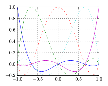
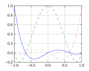
Figure 1: Lagrange basis polynomials of $\mathbb{Q}_{4}(I)$ for the Gauss-Lobatto nodes (left), corresponding basis polynomials of $V_{h}^{2,4}(I)$ (right)

As an application we investigate some properties of the so-called fluctuation operator, see the definition below. These results are important in the numerical analysis of discontinuous Galerkin methods for conservation laws.

DEFINITION 8

Let $\{\mathcal{B}_{j}\}_{1\leq j\leq n_{\rm dof}^{k}}$ be an embedded hierarchical nodal basis of degree $K,$ $K\in\mathbb{N}_{0}.$ For $\mathcal{Q}_{k}(T)=V_{h}^{K,k}(T)\oplus V_{h}^{\prime}(T),$ where $V_{h}^{K,k}(T):=\mathop{\rm span}\mathcal{B}_{K}$ and $V_{h}^{\prime}(T):=\mathop{\rm span}\{\mathcal{B}_{k}\setminus\mathcal{B}_{K}\},$ the projector $P_{h}^{K,k}:\;L^{2}(T)\to V_{h}^{K,k}(T)$ is defined by

$$(v-P_{h}^{K,k}v,w)_{0,T,h}=0\quad\forall w\in V_{h}^{K,k}(T).$$ (23)

The operator $P_{h}^{\prime}(T):=Id-P_{h}^{K,k}$ in $L^{2}(T),$ where $Id$ denotes the identity in $L^{2}(T),$ is called fluctuation operator.

LEMMA 12

Let $\{\mathcal{B}_{j}\}_{1\leq j\leq n_{\rm dof}^{k}}$ be an embedded hierarchical nodal basis of degree $K,$ $K\in\mathbb{N}_{0},$ consisting of Lagrange polynomials and suppose $\mathcal{N}=\mathcal{Q}.$ Then there is a constant $C>0$ independent of $h_{T}$ such that

$$|v-P_{h}^{K,k}v|_{r,2,T} \leq Ch_{T}^{l-r}\left[|v|_{l,2,T}+|P_{h}^{K}v|_{l,2,T}\right],\quad 0\leq r\leq l,$$

$$|v-P_{h}^{K,k}v|_{r,2,E} \leq Ch_{T}^{l-1/2-r}\left[|v|_{l,2,T}+|P_{h}^{K}v|_{l,2,T}\right],\quad 0\leq r<l-1/2$$

for all $v\in W^{l,2}(T).$

Proof: Under the above assumptions we have, for all Lagrange basis polynomials $\varphi_{j}^{K,k}\in\mathcal{B}_{k},$ that $\varphi_{j}^{K,k}(x_{i})=\delta_{ij},$ $1\leq i,j\leq n_{\rm dof}^{K},$ $x_{i}\in N(\tilde{\mathcal{B}}_{K})=N(\mathcal{B}_{K}).$ The definition of the projector $P_{h}^{K,k}$ and the property

$$w\in V_{h}^{K,k}(T)\ \Longrightarrow\ w(x_{i})=0,\quad x_{i}\in N(\mathcal{B}_{k})\setminus N(\mathcal{B}_{K})$$ (24)

imply that

$$0 \stackrel{{\scriptstyle!}}{{=}} (v-P_{h}^{K,k}v,w)_{0,T,h}=\sum_{i=1}^{n_{\rm dof}^{k}}\omega_{i}\left\{v(x_{i})-(P_{h}^{K,k}v)(x_{i})\right\}w(x_{i})$$

$$\stackrel{{\scriptstyle(\ref{eq:fop1})}}{{=}} \sum_{i=1}^{n_{\rm dof}^{K}}\omega_{i}\left\{v(x_{i})-(P_{h}^{K,k}v)(x_{i})\right\}w(x_{i})$$

and, thus,

$$v(x_{i})\stackrel{{\scriptstyle!}}{{=}}\sum_{j=1}^{n_{\rm dof}^{K}}(P_{h}^{K,k}v)_{j}\varphi_{j}^{K,k}(x_{i})\stackrel{{\scriptstyle\mathcal{N}=\mathcal{Q}}}{{=}}(P_{h}^{K,k}v)_{i},\quad 1\leq i\leq n_{\rm dof}^{K}\,.$$ (25)

As a consequence, if $I_{h}^{K}$ denotes the Lagrange interpolation operator w.r.t. the nodes $N(\mathcal{B}_{K}),$ we obtain the relation

$$I_{h}^{K}(P_{h}^{K,k}v)=\sum_{i=1}^{n_{\rm dof}^{K}}(P_{h}^{K,k}v)(x_{i})\varphi_{i}^{K}=\sum_{i,j=1}^{n_{\rm dof}^{K}}(P_{h}^{K,k}v)_{j}\varphi_{j}^{K,k}(x_{i})\varphi_{i}^{K}=\sum_{i=1}^{n_{\rm dof}^{K}}(P_{h}^{K,k}v)_{i}\varphi_{i}^{K}\stackrel{{\scriptstyle(\ref{eq:fop2})}}{{=}}I_{h}^{K}(v)\,.$$

It can be used, together with Lemma 3, in the estimation of the projection error as follows:

$$|v-P_{h}^{K,k}v|_{r,2,T} \leq |v-I_{h}^{K}v|_{r,2,T}+|I_{h}^{K}v-P_{h}^{K,k}v|_{r,2,T}$$

$$\leq |v-I_{h}^{K}v|_{r,2,T}+|P_{h}^{K,k}v-I_{h}^{K}(P_{h}^{K,k})v|_{r,2,T}\,.\quad\nolinebreak\mbox{$\blacktriangleleft$}$$

LEMMA 13

Let $\{\mathcal{B}_{j}\}_{1\leq j\leq n_{\rm dof}^{k}}$ be an embedded hierarchical nodal basis of degree $K,$ $K\in\mathbb{N}_{0},$ consisting of Lagrange polynomials and suppose $\mathcal{N}=\mathcal{Q}.$ Then:

1. $P_{h}^{K,k}$ is a linear operator,

2. $\|P_{h}^{K,k}v\|\leq C(K,k,\|\cdot\|)\|v\|_{0,\infty,T}$ for an arbitrary norm $\|\cdot\|$ on $V_{h}^{K,k}(T).$

3. For $m\in\mathbb{N},$ $v\in\mathbb{Q}_{k}(T),$ the following estimate is valid:

   $$(P_{h}^{\prime}(\nabla v),P_{h}^{\prime}(\nabla v^{2m-1}))_{0,T,h}\geq 0.$$

Proof: The assertion (i) easily follows from (25):

$$P_{h}^{K,k}(\alpha v+\beta w)=\sum_{i=1}^{n_{\rm dof}^{K}}\left[\alpha v(x_{i})+\beta w(x_{i})\right]\varphi_{i}^{K,k}=\alpha P_{h}^{K,k}v+\beta P_{h}^{K,k}w\,.$$

Item (ii) results from the estimates

$$\|P_{h}^{K,k}v\| \leq \sum_{i=1}^{n_{\rm dof}^{K}}\|v(x_{i})\varphi_{i}^{K,k}\|\leq\sum_{i=1}^{n_{\rm dof}^{K}}|v(x_{i})|\|\varphi_{i}^{K,k}\|$$

$$\leq \left(\sum_{i=1}^{n_{\rm dof}^{K}}\|\varphi_{i}^{K,k}\|\right)\|v\|_{0,\infty,T}\leq C(K,k,\|\cdot\|)\|v\|_{0,\infty,T}\,.$$

To verify (iii), we mention the following elementary inequality on $T$ ($p:=2m$):

$$\nabla v\cdot\nabla v^{p-1}=\frac{4(p-1)}{p^{2}}\nabla v^{p/2}\cdot\nabla v^{p/2}\geq 0\,.$$

Then

$$(P_{h}^{\prime}(\nabla v),P_{h}^{\prime}(\nabla v^{p-1}))_{0,T,h} \stackrel{{\scriptstyle(\ref{L2_embproj})}}{{=}} (\nabla v,\nabla v^{p-1})_{0,T,h}-(P_{h}^{K,k}(\nabla v),P_{h}^{K,k}(\nabla v^{p-1}))_{0,T,h}$$

$$\stackrel{{\scriptstyle(\ref{eq:fop2})}}{{=}} \sum_{i=1}^{n_{\rm dof}^{k}}\omega_{i}^{J}\nabla v(x_{i})\cdot\nabla v^{p-1}(x_{i})-\sum_{i=1}^{n_{\rm dof}^{K}}\omega_{i}^{J}\nabla v(x_{i})\cdot\nabla v^{p-1}(x_{i})$$

$$= \sum_{i=n_{\rm dof}^{K}+1}^{n_{\rm dof}^{k}}\omega_{i}^{J}\nabla v(x_{i})\cdot\nabla v^{p-1}(x_{i})$$

$$= \frac{4(p-1)}{p^{2}}\sum_{i=n_{\rm dof}^{K}+1}^{n_{\rm dof}^{k}}\omega_{i}^{J}\nabla v^{p/2}(x_{i})\cdot\nabla v^{p/2}(x_{i})\geq 0\,.$$

Interchanging the roles of $P_{h}^{\prime}$ and $P_{h}^{K,k},$ we obtain analogously $(P_{h}^{K,k}(\nabla v),P_{h}^{K,k}(\nabla v^{2m-1}))_{0,T,h}\geq 0.$ $\blacktriangleleft$

Motivated by Lemma 12 and the error estimate (21) we investigate the local interpolation error of the Gauss-Lobatto interpolation operator.

LEMMA 14

Let $T$ be an element of an affine partition $\mathcal{T}_{h}$ such that the corresponding family of partitions $\{\mathcal{T}_{h}\}_{h>0}$ is locally quasiuniform. Assume that $1\leq l\leq k+1,$ $l\in\mathbb{N},$ $0\leq r\leq 1$ and $2l>d+r.$ Then, for the Lagrange interpolation operator $I_{GL}^{k},$ there exist constants $C>0$ independent of $h_{T}$ and $k$ such that

$$|v-I_{GL}^{k}v|_{r,2,T} \leq C\left(\frac{h_{T}}{k}\right)^{l-r}|v|_{l,2,T},$$ (26)

$$|v-I_{GL}^{k}v|_{r,2,E} \leq C\left(\frac{h_{T}}{k}\right)^{l-1/2-r}|v|_{l,2,T}$$ (27)

for all $v\in W^{l,2}(T).$

Proof: Using Lemma 9, the proof of (26) runs analogously to the proofs of Lemmata 3 and 5.

To prove (27), we make use of the fact that, for tensor product elements, the restriction of the Gauss-Lobatto interpolant to a face $E$ of $T$ is a $(d-1)$-dimensional Gauss-Lobatto interpolant. From Lemma 9 we see that

$$|\hat{v}-\hat{I}_{GL}^{k}\hat{v}|_{r,2,\hat{E}}\leq Ck^{r-\tilde{l}}\|\hat{v}\|_{l,2,\hat{E}}$$

for all $\hat{v}\in W^{\tilde{l},2}(\hat{E})$ and all real numbers $r$ and $\tilde{l}$ such that $0\leq r\leq 1,$ $2\tilde{l}>d-1+r.$

The trace theorem (cf. (16) in the proof of Lemma 5) leads to

$$\|\hat{v}\|_{\tilde{l},2,\hat{E}}\leq C\|\hat{v}\|_{\tilde{l}+1/2,2,\hat{T}}.$$

If in addition $l=\tilde{l}+1/2\in\mathbb{N},$ the Deny-Lions lemma ([Cia91, Thm. 14.1]) implies that

$$|\hat{v}-\hat{I}_{GL}^{k}\hat{v}|_{r,2,\hat{E}}\leq Ck^{r-l+1/2}|\hat{v}|_{l,2,\hat{T}}.$$

Turning back to the original variables, we obtain (27). $\blacktriangleleft$

COROLLARY 3

Let $1\leq l\leq K+1.$ Under the assumptions of Lemmata 12 and 14, there exist constants $C>0$ independent of $h_{T}$ and $k$ such that

$$|v-P_{GL}^{K,k}v|_{r,2,T} \leq C\left(\frac{h_{T}}{K}\right)^{l-r}\left[|v|_{l,2,T}+|P_{GL}^{K}v|_{l,2,T}\right],$$

$$|v-P_{GL}^{K,k}v|_{r,2,E} \leq C\left(\frac{h_{T}}{K}\right)^{l-1/2-r}\left[|v|_{l,2,T}+|P_{GL}^{K}v|_{l,2,T}\right]$$

for all $v\in W^{l,2}(T).$

REMARK 4

As in the proof of Lemma 12, the error estimate will be reduced to an estimate of a suitable seminorm.

In general, the operators $\nabla$ and $I_{GL}^{k}$do not commute. An estimate of the commutation error is given in the next result.

LEMMA 15

Under the assumptions of Lemma 14, there exists a constant $C>0$ independent of $h_{T}$ and $k$ such that

$$\|I_{GL}^{k}(\nabla v)-\nabla I_{GL}^{k}v\|_{0,2,T,GL}\leq C\left(\frac{h_{T}}{k}\right)^{l-1}|v|_{l,2,T}.$$

Proof:

$$\|I_{GL}^{k}(\nabla v)-\nabla I_{GL}^{k}v\|_{0,2,T,GL} \stackrel{{\scriptstyle(\ref{normaeq_lumping_eq})}}{{\leq}} C\|I_{GL}^{k}(\nabla v)-\nabla I_{GL}^{k}v\|_{0,2,T}$$

$$\leq C\|\nabla(v-I_{GL}^{k}v)\|_{0,2,T}+C\|\nabla v-I_{GL}^{k}(\nabla v)\|_{0,2,T}$$

$$\stackrel{{\scriptstyle(\ref{eq:IGLkerror1})}}{{\leq}} C\left(\frac{h_{T}}{k}\right)^{l-1}|v|_{l,2,T}+C\left(\frac{h_{T}}{k}\right)^{l-1}|\nabla v|_{l-1,2,T}$$

$$\leq C\left(\frac{h_{T}}{k}\right)^{l-1}|v|_{l,2,T}.\qquad\nolinebreak\mbox{$\blacktriangleleft$}$$

6 Inverse inequalities

Inverse inequalities are an important tool in the analysis of finite element methods. Using particular properties if the tensor product representation, in this section we derive sharp inverse inequalities such that, with exception of the difference of the derivative orders and the spatial dimension, all other information is known explicitly. It is well-known that in the Nikolski inequality the dependence of the degree of polynomials cannot be improved, as the example

$$p(x)=\left(\frac{1-T_{n}^{2}(x)}{1-x^{2}}\right)^{2}$$ (28)

with $T_{n}$ being the $n$-th Čebyšov polynomial of the first kind demonstrates, see [Tim63, p. 263] (although in other papers, e.g. [GNP08, Lemma 2.4] or [CB93, Lemma 1], different statements can be found). The representation

$$T_{n}(x)=\frac{1}{2}\left[(x+\sqrt{x^{2}-1})^{n}+(x-\sqrt{x^{2}-1})^{n}\right],$$

shows that $1-T_{n}^{2}(x)$ has the zeros $-1$ and $1,$ thus (28) is really a polynomial.

Now we present a generalization of Nikolski and Markov inequalities (see [Nik51], [HST37, Sect. III]) to the tensor product situation, and we include it into the proof of an inverse inequality given in [EG04, Lemma 1.138].

Throughout this section we restrict ourselves to the case $k\geq 1.$

LEMMA 16 (local inverse inequality)

Given a reference element $\{\hat{T},\hat{P},\hat{\Sigma}\}$ such that, for $l\geq 0,$ the embedding $\hat{P}\subset W^{l,\infty}(\hat{T})$ is satisfied. Let $\{\mathcal{T}_{h}\}_{h\in(0,1]}$ be a locally quasiuniform family of affine partitions. If $0\leq m\leq l,$ then there exist

1. for $1\leq p,q\leq\infty$ a constant $C=C(l,m,p,q,d,\sigma_{0},\hat{T},P(\hat{T}))>0$ such that

   $$\|v\|_{l,p,T}\leq Ch_{T}^{m-l+d(\frac{1}{p}-\frac{1}{q})}\|v\|_{m,q,T}\qquad\forall v\in P(T),$$ (29)

2. for $1\leq q\leq p\leq\infty$ and $\hat{P}:=\mathbb{Q}_{k}(\hat{T})$ a constant $C=C(l,m,p,d,\sigma_{0})>0$ such that

   $$\|v\|_{l,p,T}\leq C\left(\frac{h_{T}}{k^{2}}\right)^{m-l}\left(\frac{h_{T}}{2(q+1)k^{2}}\right)^{d(\frac{1}{p}-\frac{1}{q})}\|v\|_{m,q,T}\qquad\forall v\in P(T).$$ (30)

The proof will be given after the presentation of the above mentioned Nikolski and Markov inequalities.

LEMMA 17 (Nikolski)

For $0<q\leq p\leq\infty$ and $\hat{v}\in\mathbb{Q}_{k}(\hat{T}),$ the following estimate is valid:

$$\|\hat{v}\|_{0,p,\hat{T}}\leq\left((q+1)k^{2}\right)^{-d(1/p-1/q)}\|\hat{v}\|_{0,q,\hat{T}}.$$ (31)

Proof: Due to [DL93, Thm. 4.2.6], in the one-dimensional situation we have the following inequality:

$$\|\hat{v}\|_{0,p,I}\leq\left((q+1)k^{2}\right)^{-(1/p-1/q)}\|\hat{v}\|_{0,q,I}\quad\forall\hat{v}\in\mathbb{Q}_{k}(I),$$

where, as above, $I=[-1,1].$ Then, for $1\leq i\leq d,$ we also have that

$$\begin{array}[]{rcl}&&\|\hat{v}(\hat{x}_{1},\dots,\hat{x}_{i-1},\cdot,\hat{x}_{i+1},\dots,\hat{x}_{d})\|_{0,\infty,I}\\ &\leq&\left((q+1)k^{2}\right)^{1/q}\|\hat{v}(\hat{x}_{1},\dots,\hat{x}_{i-1},\cdot,\hat{x}_{i+1},\dots,\hat{x}_{d})\|_{0,q,I}.\end{array}$$

A successive application of this inequality leads to

$$\begin{array}[]{rcl}\|\hat{v}\|_{0,\infty,\hat{T}}^{q}&=&\max\limits_{\hat{x}_{1}\in I}\cdots\max\limits_{\hat{x}_{d}\in I}|\hat{v}(\hat{x}_{1},\dots,\hat{x}_{d})|^{q}\\ &\leq&\max\limits_{\hat{x}_{1}\in I}\cdots\max\limits_{\hat{x}_{d-1}\in I}((q+1)k^{2})\int_{I}|\hat{v}(\hat{x}_{1},\dots,\hat{x}_{d})|^{q}d\hat{x}_{d}\\ &\leq&((q+1)k^{2})\max\limits_{\hat{x}_{1}\in I}\cdots\max\limits_{\hat{x}_{d-2}\in I}\int_{I}\max\limits_{\hat{x}_{d-1}}|\hat{v}(\hat{x}_{1},\dots,\hat{x}_{d})|^{q}\,d\hat{x}_{d}\\ &\leq&((q+1)k^{2})^{2}\max\limits_{\hat{x}_{1}\in I}\cdots\max\limits_{\hat{x}_{d-2}\in I}\int_{I}\int_{I}|\hat{v}(\hat{x}_{1},\dots,\hat{x}_{d})|^{q}\,d\hat{x}_{d-1}d\hat{x}_{d}\\ &\leq&\cdots\leq((q+1)k^{2})^{d}\|\hat{v}\|_{0,q,\hat{T}}^{q},\quad 0<q<\infty.\\ \end{array}$$

It remains to make use of an $L^{p}$-type interpolation inequality (see, e.g., [EG04, Cor. B.7]):

$$\begin{array}[]{rcl}\|\hat{v}\|_{0,p,\hat{T}}&\leq&\|\hat{v}\|_{0,q,\hat{T}}^{\frac{q}{p}}\|\hat{v}\|_{0,\infty,\hat{T}}^{1-\frac{q}{p}}\\ &\leq&\|\hat{v}\|_{0,q,\hat{T}}^{\frac{q}{p}}\left((q+1)k^{2}\right)^{\frac{d}{q}(1-\frac{q}{p})}\|\hat{v}\|_{0,q,\hat{T}}^{1-\frac{q}{p}}\\ &\leq&\left((q+1)k^{2}\right)^{-d(\frac{1}{p}-\frac{1}{q})}\|\hat{v}\|_{0,q,\hat{T}},\quad 0<q\leq p\leq\infty.\qquad\nolinebreak\mbox{$\blacktriangleleft$}\end{array}$$

LEMMA 18 (generalized Markov inequality)

For $v\in\mathbb{Q}_{k}(I)$ and $p\geq 1,$ the following estimate is valid:

$$\|v^{\prime}\|_{0,p,I}\leq C_{M}(p)k^{2}\|v\|_{0,p,I},$$

where

$$C_{M,p}=C_{M}(p):=2(p-1)^{1/p-1}\left(p+\frac{1}{k}\right)\left(1+\frac{p}{kp-p+1}\right)^{k-1+1/p}.$$

For $p=\infty,$ we even have that $\displaystyle C_{M,\infty}=1<\lim_{p\to\infty}C_{M}(p)=2e.$ Furthermore, $\forall p\in\mathbb{N}:C_{M}(p)\leq C_{M}:=6e^{1+1/e}.$

Proof: For $1<p<\infty,$ the assertion is proved in [HST37, Sect. III]. The estimate $C_{M}(p)\leq C_{M}=6e^{1+1/e}$ for all $p\in\mathbb{N}$ can be found in [MMR94, p. 590]. For $p=\infty,$ the result follows from [DL93, Thm. 4.1.4]. $\blacktriangleleft$

REMARK 5

The constants $C_{M}(p)$ can be improved. For instance, in [Bar98, Cor. 2.10] the existence of a constant $\tilde{C}_{M}(p)$ such that $\lim\limits_{p\to\infty}\tilde{C}_{M}(p)=1,$ $p>2$ is demonstrated.

COROLLARY 4

For $1\leq p\leq\infty$ and $\hat{v}\in\mathbb{Q}_{k}(\hat{T}),$ the following estimate is valid:

$$\|\hat{v}\|_{l,p,\hat{T}}\leq{d+l\choose l}^{\frac{1}{p}}\left(C_{M,p}\,k^{2}\right)^{l}\|\hat{v}\|_{0,p,\hat{T}}$$ (32)

(with the constant $C_{M,p}$ as in Lemma 18).

Proof: Iterating over the order of derivatives, it is sufficient to verify the estimate

$$\|\partial^{\alpha}\hat{v}\|_{0,p,\hat{T}}\leq(C_{M,p}k^{2})^{|\alpha|}\|\hat{v}\|_{0,p,\hat{T}}$$

for $|\alpha|=1.$ To do so, set $\alpha:=e_{i},$ where $e_{i}$ denotes the $i$-th coordinate unit vector.

For $p<\infty$ and $1\leq i\leq d$ the generalized Markov inequality implies that

$$\begin{array}[]{rcl}&&\|\hat{v}^{\prime}(\hat{x}_{1},\dots,\hat{x}_{i-1},\cdot,\hat{x}_{i+1},\dots,\hat{x}_{d})\|_{0,p,I}^{p}\\ &\leq&C_{M,p}^{p}k^{2p}\|\hat{v}(\hat{x}_{1},\dots,\hat{x}_{i-1},\cdot,\hat{x}_{i+1},\dots,\hat{x}_{d})\|_{0,p,I}^{p},\end{array}$$

hence, on $\hat{T},$

$$\begin{array}[]{rcl}\|\partial^{\alpha}\hat{v}\|_{0,p,\hat{T}}^{p}&=&\int_{I}\dots\int_{I}|\partial_{i}\hat{v}(\hat{x})|^{p}\,d\hat{x}_{i}d\hat{x}_{1}\dots d\hat{x}_{i-1}d\hat{x}_{i+1}\dots d\hat{x}_{d}\\ &\leq&C_{M,p}^{p}k^{2p}\|\hat{v}\|_{0,p,\hat{T}}^{p}.\end{array}$$

For $p=\infty,$ there is a point $\hat{y}\in\hat{T}$ such that

$$\begin{array}[]{rcl}\|\partial^{\alpha}\hat{v}\|_{0,\infty,\hat{T}}&=&|\partial_{i}\hat{v}(\hat{y})|=\max\limits_{\hat{x}_{i}\in I}|\partial_{i}\hat{v}(\hat{y}_{1},\dots,\hat{y}_{i-1},\hat{x}_{i},\hat{y}_{i+1},\dots,\hat{y}_{d})|\\ &\leq&C_{M,\infty}k^{2}\|\hat{v}(\hat{y}_{1},\dots,\hat{y}_{i-1},\cdot,\hat{y}_{i+1},\dots,\hat{y}_{d})\|_{0,\infty,I}\\ &\leq&C_{M,\infty}k^{2}\|\hat{v}\|_{0,\infty,\hat{T}}.\end{array}$$

Consequently,

$$\begin{array}[]{rcl}\|\hat{v}\|_{l,p,\hat{T}}^{p}&=&\sum_{i=0}^{l}\sum_{|\alpha|=i}\|\partial^{\alpha}\hat{v}\|_{0,p,\hat{T}}^{p}\leq\sum_{i=0}^{l}\sum_{|\alpha|=i}\left(C_{M,p}k^{2}\right)^{|\alpha|p}\|\hat{v}\|_{0,p,\hat{T}}^{p}\\ &=&\sum_{i=0}^{l}{d+i-1\choose i}\left(C_{M,p}k^{2}\right)^{ip}\|\hat{v}\|_{0,p,\hat{T}}^{p}\\ &\leq&{d+l\choose l}\left(C_{M,p}k^{2}\right)^{lp}\|\hat{v}\|_{0,p,\hat{T}}^{p},\end{array}$$

and

$$\begin{array}[]{rcl}\|\hat{v}\|_{l,\infty,\hat{T}}&=&\max\limits_{0\leq|\alpha|\leq l}\|\partial^{\alpha}\hat{v}\|_{0,\infty,\hat{T}}\leq\max\limits_{0\leq|\alpha|\leq l}\left(C_{M,\infty}k^{2}\right)^{|\alpha|}\|\hat{v}\|_{0,\infty,\hat{T}}\\ &\leq&\left(C_{M,\infty}k^{2}\right)^{l}\|\hat{v}\|_{0,\infty,\hat{T}}.\qquad\nolinebreak\mbox{$\blacktriangleleft$}\end{array}$$

Now we are ready to prove the inverse estimates (29) and (30).

Proof of Lemma 16:

The first estimate is proved along the lines of the proof of [EG04, Lemma 1.138]. In the particular case of a Lagrange reference element we use the same idea of proof but make use of the results prepared in this section.

As usual, first the assertion is proved for $m=0.$ By $(\ref{inv_l_0})$ and $(\ref{nikolskii_ungleichung}),$ on $\hat{T}$ we have that

$$\|\hat{v}\|_{l,p,\hat{T}}\leq{d+l\choose l}^{\frac{1}{p}}\left(C_{M,p}k^{2}\right)^{l}\left((q+1)k^{2}\right)^{-d(\frac{1}{p}-\frac{1}{q})}\|\hat{v}\|_{0,q,\hat{T}}.$$ (33)

In order to get the corresponding estimate for the transformed element $T,$ we make use of $(\ref{trans_ungl2}),$ $(\ref{help_scaling2})$ and $(\ref{help_scaling3})$ for $0\leq j\leq l:$

$$\begin{array}[]{rcl}|v|_{j,p,T}^{p}&\leq&\left\{C_{j,d}\|J_{T}^{-1}\|_{\ell^{2}}^{j}|\det J_{T}|^{1/p}\right\}^{p}|\hat{v}|_{j,p,\hat{T}}^{p}\\ &\leq&\left\{C_{j,d}\left(2\sqrt{d}\sigma_{0}h_{T}^{-1}\right)^{j}\left(\frac{h_{T}}{2}\right)^{\frac{d}{p}}\right\}^{p}\|\hat{v}\|_{j,p,\hat{T}}^{p}\\ &\stackrel{{\scriptstyle(\ref{inv_ref})}}{{\leq}}&\left\{{d+j\choose j}^{\frac{1}{p}}\tilde{C}(j,p,d,\sigma_{0})\left(\frac{h_{T}}{k^{2}}\right)^{-j}\left(\frac{h_{T}}{2}\right)^{\frac{d}{p}}\left((q+1)k^{2}\right)^{-d(\frac{1}{p}-\frac{1}{q})}\right\}^{p}\|\hat{v}\|_{0,q,\hat{T}}^{p},\end{array}$$

where $\tilde{C}(j,p,d,\sigma_{0})=C_{j,d}\left(2\sqrt{d}\sigma_{0}C_{M,p}\right)^{j}.$ By $(\ref{trans_ungl1})$ with $l=0,$ the back-transformation yields

$$|v|_{j,p,T}\leq{d+j\choose j}^{\frac{1}{p}}\tilde{C}(j,p,d,\sigma_{0})\left(\frac{h_{T}}{k^{2}}\right)^{-j}\left(\frac{h_{T}}{2(q+1)k^{2}}\right)^{d(\frac{1}{p}-\frac{1}{q})}\|v\|_{0,q,T}.$$

Under the assumption $h_{T}^{-1}\geq 1$ for $0\leq j\leq l,$ the corresponding Sobolev norm can be estimated as

$$\begin{array}[]{rcl}\|v\|_{j,p,T}^{p}&=&\sum_{s=0}^{j}|v|_{s,p,T}^{p}\\ &\leq&\sum_{s=0}^{j}{d+s\choose s}\left\{\tilde{C}(s,p,d,\sigma_{0})\left(\frac{h_{T}}{k^{2}}\right)^{-s}\left(\frac{h_{T}}{2(q+1)k^{2}}\right)^{d(\frac{1}{p}-\frac{1}{q})}\right\}^{p}\|v\|_{0,q,T}^{p}\\ &\leq&{d+1+j\choose j}\left\{\tilde{C}(j,p,d,\sigma_{0})\left(\frac{h_{T}}{k^{2}}\right)^{-j}\left(\frac{h_{T}}{2(q+1)k^{2}}\right)^{d(\frac{1}{p}-\frac{1}{q})}\right\}^{p}\|v\|_{0,q,T}^{p},\end{array}$$ (34)

and the assertion is proved for $m=0.$ Now, let $0\leq m\leq l$ and $\alpha$ be a multiindex with $0\leq|\alpha|\leq l.$ In the case $|\alpha|\leq l-m,$ the estimate $(\ref{inv_m_0})$ and the relation

$$\|\partial^{\alpha}v\|_{0,p,T}^{p}\leq\sum_{|\alpha|\leq l-m}\|\partial^{\alpha}v\|_{0,p,T}^{p}=\|v\|_{l-m,p,T}^{p}$$

imply that

$$\begin{array}[]{rcl}\|\partial^{\alpha}v\|_{0,p,T}&\leq&C(l-m,p,d,\sigma_{0})\left(\frac{h_{T}}{k^{2}}\right)^{m-l}\left(\frac{h_{T}}{2(q+1)k^{2}}\right)^{d(\frac{1}{p}-\frac{1}{q})}\|v\|_{0,q,T}\\ &\leq&C(l-m,p,d,\sigma_{0})\left(\frac{h_{T}}{k^{2}}\right)^{m-l}\left(\frac{h_{T}}{2(q+1)k^{2}}\right)^{d(\frac{1}{p}-\frac{1}{q})}\|v\|_{m,q,T},\end{array}$$

where $C(j,p,d,\sigma_{0}):={d+1+j\choose j}^{1/p}\tilde{C}(j,p,d,\sigma_{0}).$ This inequality is also valid for $l-m\leq|\alpha|\leq l,$ because there exist two further multiindices $\beta$ and $\gamma$ such that $\alpha=\beta+\gamma,$ $|\beta|=l-m$ and $|\gamma|\leq m.$ As in the first case we get

$$\begin{array}[]{rcl}\|\partial^{\alpha}v\|_{0,p,T}&=&\|\partial^{\beta}\left(\partial^{\gamma}v\right)\|_{0,p,T}\\ &\leq&C(l-m,p,d,\sigma_{0})\left(\frac{h_{T}}{k^{2}}\right)^{m-l}\left(\frac{h_{T}}{2(q+1)k^{2}}\right)^{d(\frac{1}{p}-\frac{1}{q})}\|\partial^{\gamma}v\|_{0,q,T}\\ &\leq&C(l-m,p,d,\sigma_{0})\left(\frac{h_{T}}{k^{2}}\right)^{m-l}\left(\frac{h_{T}}{2(q+1)k^{2}}\right)^{d(\frac{1}{p}-\frac{1}{q})}\|v\|_{m,q,T}.\end{array}$$

Since this estimate is valid for $0\leq|\alpha|\leq l,$ the norm $\|v\|_{l,p,T}^{p}$ can be estimated by using its definition, and the statement follows with

$$C(l,m,p,d,\sigma_{0}):=C_{l-m,d}\left(2\sqrt{d}\sigma_{0}C_{M,p}\right)^{l-m}{d+1+l-m\choose l-m}^{1/p}{d+l\choose l}^{1/p}.$$

The equality sign occurs in the case $l=m=0$ and $p=q.$ $\blacktriangleleft$

LEMMA 19 (global inverse inequality)

Under the assumptions of Lemma $\ref{inverse_estimate},$ for a locally quasiuniform family of affine partitions $\{\mathcal{T}_{h}\}_{h\in(0,1]}$ and for all $v\in W_{h},$ there exist

1. for $1\leq p,q\leq\infty$ a constant $C=C(l,m,p,q,d,\sigma_{0},\hat{T},P(\hat{T}),C_{qu})>0$ such that

   $$\Big{(}\sum_{T\in\mathcal{T}_{h}}\|v\|_{l,p,T}^{p}\Big{)}^{\frac{1}{p}}\leq Ch^{m-l+min(0,d(\frac{1}{p}-\frac{1}{q}))}\Big{(}\sum_{T\in\mathcal{T}_{h}}\|v\|_{m,q,T}^{q}\Big{)}^{\frac{1}{q}},$$

2. for $1\leq q\leq p\leq\infty$ and $\hat{P}=\mathbb{Q}_{k}(\hat{T})$ a constant $C=C(l,m,p,d,\sigma_{0})>0$

   $$\Big{(}\sum_{T\in\mathcal{T}_{h}}\|v\|_{l,p,T}^{p}\Big{)}^{\frac{1}{p}}\leq C\left(\frac{C_{qu}h}{k^{2}}\right)^{m-l}\left(\frac{C_{qu}h}{2(q+1)k^{2}}\right)^{d(\frac{1}{p}-\frac{1}{q})}\Big{(}\sum_{T\in\mathcal{T}_{h}}\|v\|_{m,q,T}^{q}\Big{)}^{\frac{1}{q}}.$$

Proof: The proof of the first estimate can be found in [EG04, Cor. 1.141]. With

$$C=C(l,m,p,d,\sigma_{0}),$$

the second estimate follows from Lemma 16 and from the quasiuniformity of $\{\mathcal{T}_{h}\}_{h>0}$:

$$\sum_{T\in\mathcal{T}_{h}}\|v\|_{l,p,T}^{p}\leq C^{p}\left(\frac{C_{qu}h}{k^{2}}\right)^{p(m-l)}\left(\frac{C_{qu}h}{2(q+1)k^{2}}\right)^{pd(\frac{1}{p}-\frac{1}{q})}\sum_{T\in\mathcal{T}_{h}}\|v\|_{m,q,T}^{p}.$$

Taking the $p$-th root, together with $\|\cdot\|_{\ell^{p}}\leq\|\cdot\|_{\ell^{q}}$ the statement follows for $p,q\neq\infty.$ The proof in the case $p=q=\infty$ immediately follows from the definitions of the norms. $\blacktriangleleft$

References

[AF03]
R.A. Adams and J.J.F. Fournier.
Sobolev spaces, volume 140 of Pure and Applied Mathematics
(Amsterdam).
Elsevier/Academic Press, Amsterdam, 2nd edition, 2003.
[Bar98]
M. Baran.
New approach to Markov inequality in norms.
In Approximation theory, volume 212 of Monogr. Textbooks
Pure Appl. Math., pages 75–85. Dekker, New York, 1998.
[BL76]
J. Bergh and J. Löfström.
Interpolation spaces. An introduction.
Springer-Verlag, Berlin, 1976.
Grundlehren der Mathematischen Wissenschaften, No. 223.
[BM97]
C. Bernardi and Y. Maday.
Spectral methods.
In Handbook of numerical analysis, Vol. V, pages 209–485.
North-Holland, Amsterdam, 1997.
[CB93]
Q. Chen and I. Babuška.
Polynomial interpolation of real functions I: Interpolation in an
interval.
Technical Note BN 1153, University of Maryland, College Park, 1993.
[CGGR00]
D. Calvetti, G.H. Golub, W.B. Gragg, and L. Reichel.
Computation of Gauss-Kronrod quadrature rules.
Math. Comp., 69(231):1035–1052, 2000.
[CHQZ07]
C. Canuto, M.Y. Hussaini, A. Quarteroni, and T.A. Zang.
Spectral methods.
Scientific Computation. Springer, Berlin, 2007.
Evolution to complex geometries and applications to fluid dynamics.
[Cia91]
P.G. Ciarlet.
Basic error estimates for elliptic problems.
In P.G. Ciarlet and J.L. Lions, editors, Handbook of numerical
analysis. II: Finite element methods (Part 1), pages 17–351. North-Holland,
Amsterdam-London-New York-Tokyo, 1991.
[CQ82]
C. Canuto and A. Quarteroni.
Approximation results for orthogonal polynomials in Sobolev spaces.
Math. Comp., 38(157):67–86, 1982.
[DL93]
R.A. DeVore and G.G. Lorentz.
Constructive approximation.
Springer-Verlag, Berlin-Heidelberg-New York, 1993.
[EG04]
A. Ern and J.-L. Guermond.
Theory and practice of finite elements, volume 159 of Applied Mathematical Sciences.
Springer-Verlag, New York, 2004.
[Fej32]
L. Fejér.
Bestimmung derjenigen Abszissen eines Intervalles, für welche
die Quadratsumme der Grundfunktionen der Lagrangeschen Interpolation
im Intervalle ein möglichst kleines Maximum besitzt.
Ann. Scuola Norm. Sup. Pisa Cl. Sci. (2), 1(3):263–276, 1932.
[Gag57]
E. Gagliardo.
Caratterizzazione delle Tracce sulla Frontiera Relative ad
Alcune Classi di Funzioni in Variabli.
Rend. Sem. Mat. Padova, 27:284–305, 1957.
[Geo03]
E.H. Georgoulis.
Discontinuous Galerkin methods on shape-regular and
anisotropic meshes.
PhD thesis, Oxford University Computing Laboratory, 2003.
[GNP08]
T. Gudi, N. Nataraj, and A.K. Pani.
-discontinuous Galerkin methods for strongly nonlinear
elliptic boundary value problems.
Numer. Math., 109(2):233–268, 2008.
[HSS02]
P. Houston, C. Schwab, and E. Süli.
Discontinuous -finite element methods for
advection-diffusion-reaction problems.
SIAM J. Numer. Anal., 39(6):2133–2163, 2002.
[HST37]
E. Hille, G. Szegö, and J.D. Tamarkin.
On some generalizations of a theorem of A. Markoff.
Duke Math. J., 3(4):729–739, 1937.
[JK95]
D. Jerison and C.E. Kenig.
The inhomogeneous Dirichlet problem in Lipschitz domains.
J. Funct. Anal., 130(1):161–219, 1995.
[Joh02]
W.P. Johnson.
The curious history of Faà di Bruno’s formula.
Amer. Math. Monthly, 109(3):217–234, 2002.
[Kal85]
G.A. Kalyabin.
Theorems on extension, multipliers and diffeomorphisms for
generalized Sobolev-Liouville classes in domains with Lipschitz
boundary.
Trudy Mat. Inst. Steklov., 172:173–186, 353, 1985.
Studies in the theory of functions of several real variables and the
approximation of functions.
[KS05]
G.E. Karniadakis and S.J. Sherwin.
Spectral/ element methods for computational fluid
dynamics.
Numerical Mathematics and Scientific Computation. Oxford University
Press, New York, 2nd edition, 2005.
[MMR94]
G.V. Milovanović, D.S. Mitrinović, and Th.M. Rassias.
Topics in polynomials: extremal problems, inequalities, zeros.
World Scientific Publishing Co. Inc., River Edge, NJ, 1994.
[Neč67]
J. Nečas.
Les méthodes directes en théorie des équations
elliptiques.
Academia, Prague, 1967.
[Nik51]
S.M. Nikolski.
Inequalities for entire functions of exponential type and their
application to the theory of differentiable functions of several variables.
In Trudy Mat. Inst. Steklova, vol. 38, pages 244–278. Izdat.
Akad. Nauk SSSR, Moscow, 1951.
English transl.: Amer. Math. Soc. Transl. 80(1969), (2), 1-38.
[QV94]
A. Quarteroni and A. Valli.
Numerical approximation of partial differential equations.
Springer-Verlag, Berlin-Heidelberg-New York, 1994.
[Ste70]
E.M. Stein.
Singular integrals and differentiability properties of
functions.
Princeton Mathematical Series, No. 30. Princeton University Press,
Princeton, N.J., 1970.
[SvdVvD06]
J.J. Sudirham, J.J.W. van der Vegt, and R.M.J. van Damme.
Space-time discontinuous Galerkin method for advection-diffusion
problems on time-dependent domains.
Appl. Numer. Math., 56(12):1491–1518, 2006.
[Tim63]
A.F. Timan.
Theory of approximation of functions of a real variable.
Translated by J.Berry.International Series of Monographs on Pure and Applied Mathematics,
vol. 34. Pergamon Press, Oxford etc., 1963.
[Tri78]
H. Triebel.
Interpolation theory, function spaces, differential operators,
volume 18 of North-Holland Mathematical Library.
North-Holland Publishing Co., Amsterdam, 1978.