Elliptic Flow: A Brief Review

Abstract

One of the fundamental questions in the field of subatomic physics is what happens to matter at extreme densities and temperatures as may have existed in the first microseconds after the Big Bang and exists, perhaps, in the core of dense neutron stars. The aim of heavy-ion physics is to collide nuclei at very high energies and thereby create such a state of matter in the laboratory. The experimental program started in the 1990’s with collisions made available at the Brookhaven Alternating Gradient Synchrotron (AGS), the CERN Super Proton Synchrotron (SPS) and continued at the Brookhaven Relativistic Heavy-Ion Collider (RHIC) with maximum center of mass energies of $\sqrt{s_{{}_{\rm NN}}}$ = 4.75, 17.2 and 200 GeV respectively. Collisions of heavy-ions at the unprecedented energy of 2.76 TeV have recently become available at the LHC collider at CERN. In this review I will give a brief introduction to the physics of ultra-relativistic heavy-ion collisions and discuss the current status of elliptic flow measurements.

1 Heavy-Ion Physics

To our current understanding, the universe went through a series of phase transitions which mark the most important epochs of the expanding universe after the Big Bang. At $10^{-11}$ s and at a temperature of $T\sim$ 100 GeV ($\sim 10^{15}$ K) the electroweak phase transition took place where most of the known elementary particles acquired their Higgs masses [1, 2, 3]. At $10^{-5}$ s and at a temperature of $\sim 200$ MeV ($\sim 10^{12}$ K), the strong phase transition took place where the quarks and gluons became confined into hadrons and where the approximate chiral symmetry was spontaneously broken [4].

Quantum Chromodynamics (QCD) is the underlying theory of the strong force. Although its fundamental degrees of freedom (quarks and gluons) cannot be observed as free particles the QCD Lagrangian is well established. One of the key features of QCD is the self coupling of the gauge bosons (gluons) which cause the coupling constant to increase with decreasing momentum transfer. This running of the coupling constant gives rise to asymptotic freedom [5, 6] and confinement at large and small momentum transfers, respectively. At small momentum transfer nonperturbative corrections, which are notoriously hard to calculate, become important. For this reason two important nonperturbative properties of QCD, confinement and chiral symmetry breaking, are still poorly understood from first principles.

One of the fundamental questions in QCD phenomenology is what the properties of matter are at the extreme densities and temperatures where the quarks and gluons are in a deconfined state, the so-called Quark Gluon Plasma (QGP) [7]. Basic arguments [7] allow us to estimate the energy density $\epsilon\sim$ 1 GeV/fm³ and temperature $T\sim$ 200 MeV at which the strong phase transition takes place. These values imply that the transition occurs in a regime where the coupling constant is large so that we can not rely anymore on perturbative QCD. Better understanding of the non-perturbative domain comes from lattice QCD, where the field equations are solved numerically on a discrete space-time grid. Lattice QCD provides quantitative information on the QCD phase transition and the Equation of State (EoS) of the deconfined state. At extreme temperatures (large momenta) we expect that the quarks and gluons are weakly interacting and that the QGP would behave as an ideal gas. For an ideal massless gas the EoS is given by:

$$P = \frac{1}{3}\epsilon,\;\;\;\epsilon=g\frac{\pi^{2}}{30}T^{4},$$ (1)

where $P$ is the pressure, $\epsilon$ the energy density, $T$ the temperature and $g$ is the effective number of degrees of freedom. Each bosonic degree of freedom contributes 1 unit to $g$, whereas each fermionic degree of freedom contributes $\frac{7}{8}$. The value of $g=47.5$ for a three flavor QGP which is an order of magnitude larger than that of a pion gas where $g\sim 3$.

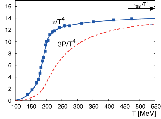
Figure 1: Energy density $\epsilon/T^{4}$ (full curve) and pressure $3P/T^{4}$ (dashed curve) as a function of temperature $T$ from lattice calculations [8]. The arrow indicates the Stefan Boltzmann limit of the energy density.

Figure 1 shows the temperature dependence of the energy density as calculated from lattice QCD [8]. It is seen that the energy density changes rapidly around $T\sim$ 190 MeV, which is due to the rapid increase in the effective degrees of freedom (lattice calculations show that the transition is a crossover). Also shown in Fig. 1 is the pressure which changes slowly compared to the rapid increase of the energy density around $T=190$ MeV. It follows that the speed of sound, $c_{\rm s}=\sqrt{\partial P/\partial\epsilon}$, is reduced during the strong phase transition. At large temperature the energy density reaches a significant fraction ($\sim 0.9$) of the ideal massless gas limit (Stefan-Boltzmann limit).

Relativistic heavy-ion collisions are a unique tool to create and study hot QCD matter and its phase transition under controlled conditions [7, 9, 10, 11, 12, 13]. As in the early universe, the hot and dense system created in a heavy-ion collision will expand and cool down. During this evolution the system probes a range of energy densities and temperatures, and possibly different phases. Provided that the quarks and gluons undergo multiple interactions the system will thermalize and form the QGP which subsequently undergoes a collective expansion and eventually becomes so dilute that it hadronizes. This collective expansion is called flow.

Flow is an observable that provides experimental information on the equation of state and the transport properties of the created QGP. The azimuthal anisotropy in particle production is the clearest experimental signature of collective flow in heavy-ion collisions [14, 15, 16, 17, 18] . This so-called anisotropic flow is caused by the initial asymmetries in the geometry of the system produced in a non-central collision. The second Fourier coefficient of the azimuthal asymmetry is called elliptic flow. In this report I will describe the relation between elliptic flow and the geometry of the collision (section 2 and 3), the sensitivity of elliptic flow to the EoS and transport properties (section 3) and the techniques used to measure elliptic flow from the data (section 4). In section 5 I will review the elliptic flow measurements at the LHC and at lower energies, together with the current theoretical understanding of these results.

2 Event Characterization

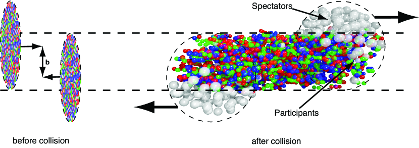
Figure 2: Left: The two heavy-ions before collision with impact parameter b. Right: The spectators continue unaffected, while in the participant zone particle production takes place.

Heavy-ions are extended objects and the system created in a head-on collision is different from that in a peripheral collision. To study the properties of the created system, collisions are therefore categorized by their centrality. Theoretically the centrality is defined by the impact parameter ${\bf b}$ (see Fig. 2) which, however, cannot be directly observed.

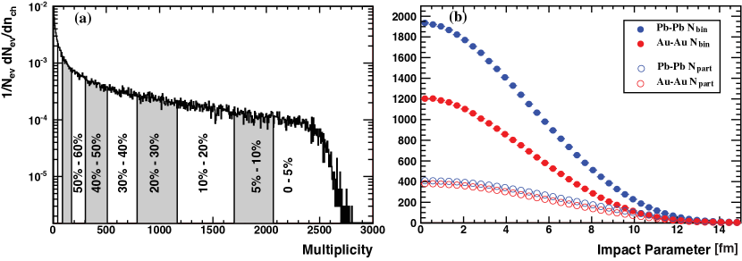
Figure 3: a) Charged particle distribution from Pb-Pb collisions at $\sqrt{s_{{}_{\rm NN}}}$ = 2.76 TeV measured with ALICE, showing a classification in centrality percentiles (from [20]). b) Number of participating nucleons $N_{\rm part}$ and binary collisions $N_{\rm bin}$ versus impact parameter for Pb-Pb and Au-Au collisions at $\sqrt{s_{{}_{\rm NN}}}$ = 2.76 and 0.2 TeV, respectively.

Experimentally, the collision centrality can be inferred from the measured particle multiplicities, given the assumption that the multiplicity is a monotonic function of ${\bf b}$. The centrality is then characterized by the fraction, $\pi b^{2}/\pi(2R_{A})^{2}$, of the geometrical cross-section with $R_{A}$ the nuclear radius (see Fig. 3a).

Instead of by impact parameter, the centrality is also often characterized by the number of participating nucleons (nucleons that undergo at least one inelastic collision) or by the number of equivalent binary collisions. Phenomenologically it is found that the total particle production scales with the number of participating nucleons whereas hard processes scale with the number of binary collisions. These measures can be related to the impact parameter ${\bf b}$ using a realistic description of the nuclear geometry in a Glauber calculation [19], as is shown in Fig. 3b. This Figure also shows that Pb–Pb collisions at $\sqrt{s_{{}_{\rm NN}}}$ = 2.76 TeV and Au-Au at $\sqrt{s_{{}_{\rm NN}}}$ = 0.2 TeV have a similar distribution of participating nucleons. The number of binary collisions increases from Au–Au to Pb–Pb by about 50% because the nucleon-nucleon inelastic cross section increases by about that amount at the respective center of mass energies of 0.2 and 2.76 TeV.

3 Anisotropic Flow

Flow signals the presence of multiple interactions between the constituents of the medium created in the collision. More interactions usually leads to a larger magnitude of the flow and brings the system closer to thermalization. The magnitude of the flow is therefore a detailed probe of the level of thermalization.

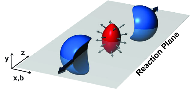
Figure 4: Almond shaped interaction volume after a non-central collision of two nuclei. The spatial anisotropy with respect to the $x$-$z$ plane (reaction plane) translates into a momentum anisotropy of the produced particles (anisotropic flow).

The theoretical tools to describe flow are hydrodynamics or microscopic transport (cascade) models. In the transport models flow depends on the opacity of the medium, be it partonic or hadronic. Hydrodynamics becomes applicable when the mean free path of the particles is much smaller than the system size, and allows for a description of the system in terms of macroscopic quantities. This gives a handle on the equation of state of the flowing matter and, in particular, on the value of the sound velocity $c_{s}$.

Experimentally, the most direct evidence of flow comes from the observation of anisotropic flow which is the anisotropy in particle momentum distributions correlated with the reaction plane. The reaction plane is defined by the impact parameter and the beam direction $z$ (see Fig. 4). A convenient way of characterizing the various patterns of anisotropic flow is to use a Fourier expansion of the invariant triple differential distributions:

$$E\frac{{\mathrm{d}}^{3}N}{{\mathrm{d}}^{3}{\bf p}}=\frac{1}{2\pi}\frac{{\mathrm{d}}^{2}N}{p_{\mathrm{t}}{\mathrm{d}}p_{\mathrm{t}}{\mathrm{d}}y}\left(1+2\sum_{n=1}^{\infty}v_{n}\cos[n(\varphi-\Psi_{\rm RP})]\right),$$ (2)

where $E$ is the energy of the particle, $p$ the momentum, $p_{\rm t}$ the transverse momentum, $\varphi$ the azimuthal angle, $y$ the rapidity, and $\Psi_{\rm RP}$ the reaction plane angle. The sine terms in such an expansion vanish because of the reflection symmetry with respect to the reaction plane. The Fourier coefficients are $p_{\mathrm{t}}$ and $y$ dependent and are given by

$$v_{n}(\mbox{$p_{\mathrm{t}}$},y)=\langle\cos[n(\varphi-\Psi_{\rm RP})]\rangle,$$ (3)

where the angular brackets denote an average over the particles, summed over all events, in the $(\mbox{$p_{\mathrm{t}}$},y)$ bin under study. In this Fourier decomposition, the coefficients $v_{1}$ and $v_{2}$ are known as directed and elliptic flow, respectively.

Figure 5: The created initial transverse energy density profile and its time dependence in coordinate space for a non-central heavy-ion collision [21]. The $z$-axis is along the colliding beams, the $x$-axis is defined by the impact parameter.

The evolution of the almond shaped interaction volume is shown in Fig. 5. The contours indicate the energy density profile and the plots from left to right show how the system evolves from an almond shaped transverse overlap region into an almost symmetric system. During this expansion, governed by the velocity of sound, the created hot and dense system cools down.

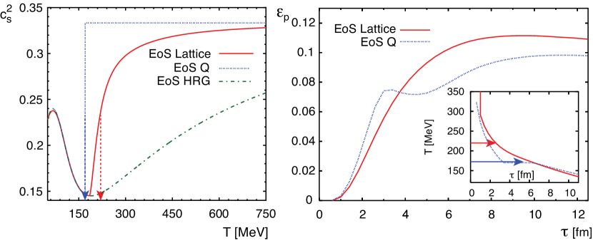
Figure 6: a) The velocity of sound squared versus temperature for three equations of state [22]. b) The anisotropy in momentum space for two equations of state used in hydrodynamic calculations [22].

Figure 6a shows the velocity of sound versus temperature for three different equations of state [22]. The dash-dotted line is the hadron resonance gas EoS, the red full line is a parameterization of the EoS which matches recent lattice calculations and the blue dashed line is an EoS which incorporates a first order phase transition. The arrows indicate the corresponding transition temperatures for the lattice inspired EoS and the EoS with a first order phase transition. The temperature dependence of the sound velocity clearly differs significantly between the different equations of state. Because the expansion of the system and the buildup of collective motion depend on the velocity of sound, it is expected that this difference will have a clear signature in the flow. The buildup of the flow for two different EoS is shown in Fig. 6b. Due to the stronger expansion in the reaction plane the initial almond shape anisotropy in coordinate space vanishes, as was shown in Fig. 5, while the momentum space distribution changes in the opposite direction from being approximately azimuthally symmetric to having a preferred direction in the reaction plane. The asymmetry in momentum space can be quantified by:

$$\varepsilon_{p}=\frac{\langle T_{xx}-T_{yy}\rangle}{\langle T_{xx}+T_{yy}\rangle},$$ (4)

where $T_{xx}$ and $T_{yy}$ are the diagonal transverse components of the energy momentum tensor and the brackets denote an averaging over the transverse plane. Figure 6b shows that $\varepsilon_{p}$ versus time starts at zero after which the anisotropy quickly develops and is indeed dependent on the EoS.

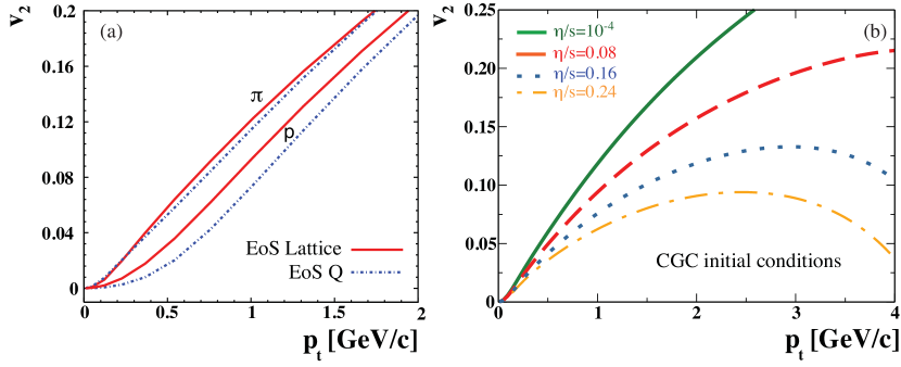
Figure 7: a) The EoS dependence of $v_{2}(\mbox{$p_{\mathrm{t}}$})$ for pions and protons [22]. The full lines are for the lattice inspired EoS and the dashed lines for an EoS which incorporates a first order phase transition. b) The dependence on $\eta$/s of $v_{2}(\mbox{$p_{\mathrm{t}}$})$ for charged particles [24].

Although $\varepsilon_{p}$ is not a direct observable, the observed EoS dependence of $\varepsilon_{p}$ versus time is reflected in the experimental observable $v_{2}$, in particular when plotted as function of transverse momentum and particle mass. Figure 7a shows $p_{\rm t}$-differential elliptic flow for pions and protons after the transverse momentum spectra have been constrained. A clear mass dependence of $v_{2}$ at low transverse momentum is observed for both equations of state. The figure also clearly shows that the pion $v_{2}$ does not change much between the lattice EoS and EoS Q. On the other hand, the $v_{2}$ of protons does change significantly because the heavier particles are more sensitive to the change in collective motion. Therefore measurements of $v_{2}(p_{t})$ for various particle species provide an excellent constraint on the EoS in ideal hydrodynamics.

More recently, it was realized that small deviations from ideal hydrodynamics, in particular viscous corrections, already modify significantly the buildup of the elliptic flow [23]. The shear viscosity determines how good a fluid is, however, for relativistic fluids the more useful quantity is the shear viscosity over entropy ratio $\eta/s$. Known good fluids in nature have an $\eta/s$ of order $\hbar/k_{\rm B}$. In a strongly coupled ${\cal N}=4$ supersymmetric Yang Mills theory with a large number of colors (’t Hooft limit), $\eta/s$ can be calculated using a gauge gravity duality [25]:

$$\frac{\eta}{s}=\frac{\hbar}{4\pi k_{\rm B}}.$$

Kovtun, Son and Starinets conjectured, using the AdS/CFT correspondence, that this implies that all fluids have $\eta/s\geq\hbar/4\pi k_{\rm B}$ (the KSS bound.). We therefore call a fluid with $\eta/s=1/4\pi$ (in natural units) a perfect fluid. The KSS bound raises the interesting question on how fundamental this value is in nature and if the QGP behaves like an almost perfect fluid. It is argued that the transition from hadrons to quarks and gluons occurs in the vicinity of the minimum in $\eta/s$, just as is the case for the phase transitions in helium, nitrogen, and water. An experimental measurement of the minimal value of $\eta/s$ would thus pinpoint the location of the transition [26, 27].

Experimentally we might get an answer to the magnitude of $\eta/s$ by measuring $v_{2}$ as is shown in Fig. 7b. The full line is close to ideal hydrodynamics ($\eta/s\sim 0$) while the three other lines correspond to $\eta/s$ values of up to three times the KSS bound. Different magnitudes of $\eta/s$ clearly lead to a dramatically different magnitude of $v_{2}$ and change its $p_{\rm t}$ dependence. However the magnitude and $p_{\rm t}$ dependence of $v_{2}$ not only depend on $\eta/s$ but also on the EoS as we have seen.

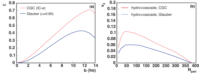
Figure 8: a) The eccentricity $\varepsilon$ calculated in a color glass condensate (CGC) model and using a Glauber model [28]. b) The $v_{2}$ obtained using the CGC or Glauber initial eccentricity [28].

The magnitude of $v_{2}$ does not only depend on the medium properties of interest, but is also proportional to the initial spatial anisotropy of the collision region. This spatial anisotropy can be characterized by the eccentricity, which is defined by

$$\varepsilon=\frac{\left<y^{2}-x^{2}\right>}{\left<y^{2}+x^{2}\right>},$$ (5)

where $x$ and $y$ are the positions of the participating nucleons in the transverse plane and the brackets denote an average which traditionally was taken over the number of participants. Recent calculations have shown that the eccentricity obtained in different descriptions, in particular comparing a Glauber with a Color Glass Condensate (CGC) description, shows that $\varepsilon$ varies by almost 25% at a given impact parameter [28], see Fig. 8a. The elliptic flow, obtained when using these different initial eccentricities is shown in Fig. 8b. As expected, the different magnitude of the eccentricity propagates to the magnitude of the elliptic flow. Because currently we cannot measure the eccentricity independently this leads to a large uncertainty in experimental determination of $\eta$/s.

To summarize, we have seen that the elliptic flow depends on fundamental properties of the created matter, in particular the sound velocity and the shear viscosity, but also on the initial spatial eccentricity. Detailed measurements of elliptic flow as function of transverse momentum, particle mass and collision centrality provide an experimental handle on these properties. In the next section, before we discuss the measurements, we first explain how we estimate the anisotropic flow experimentally.

4 Elliptic Flow: Analysis Methods

Because the reaction plane angle is not a direct observable the elliptic flow (Eq. 3) can not be measured directly so that it is usually estimated using azimuthal correlations between the observed particles. Two-particle azimuthal correlations, for example, can be written as:

$$\langle\langle e^{i2(\varphi_{1}-\varphi_{2})}\rangle\rangle = \langle\langle e^{i2(\varphi_{1}-\Psi_{\rm RP}-(\varphi_{2}-\Psi_{\rm RP}))}\rangle\rangle,$$ (6)

$$= \langle\langle e^{i2(\varphi_{1}-\Psi_{\rm RP})}\rangle\langle e^{-i2(\varphi_{2}-\Psi_{\rm RP})}\rangle+\delta_{2}\rangle,$$

$$= \langle v_{2}^{2}+\delta_{2}\rangle,$$

where the double brackets denote an average over all particles within an event, followed by averaging over all events. In Eq. 6 we have factorized the azimuthal correlation between the particles in a common correlation with the reaction plane (elliptic flow $v_{2}$) and a correlation independent of the reaction plane (non-flow $\delta_{2}$). Here we have assumed that the correlation between $v_{2}$ and $\delta_{2}$ is negligible. If $\delta_{2}$ is small, Eq. 6 can be used to measure $\left<v_{2}^{2}\right>$, but in general the non-flow contribution is not negligible.

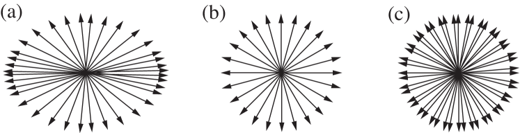
Figure 9: Examples of particle distributions in the transverse plane, where for a) $v_{2}>0$, $v_{2}\{2\}>0$, b) $v_{2}=0$, $v_{2}\{2\}=0$, and c) $v_{2}=0$, $v_{2}\{2\}>0$.

In Fig. 9 we illustrate two-particle nonflow contributions as follows: In Fig. 9a an anisotropic distribution is shown for which both $v_{2}=\langle\cos 2\phi\rangle$ and the two-particle correlation $v_{2}\{2\}=\sqrt{\langle\cos 2(\phi_{1}-\phi_{2})\rangle}$ are positive. Figure 9b shows a symmetric distribution for which $v_{2}=0$ and also $v_{2}\{2\}=0$. Figure 9c shows two symmetric distributions rotated with respect to each other which give $v_{2}=0$ while $v_{2}\{2\}$ is nonzero. This illustrates how non-flow contributions from sources like resonance decays or jets can contribute to $v_{2}$ measured from two particle correlations.

The collective nature of elliptic flow can be exploited to suppress non-flow contributions [29, 30]. This is done using so called cumulants, which are genuine multi-particle correlations. For instance, the two particle cumulant $c_{2}\{2\}$ and the four particle cumulants $c_{2}\{4\}$ are defined as:

$$c_{2}\{2\} \equiv \left<\left<e^{i2(\varphi_{1}-\varphi_{2})}\right>\right>=\left<v_{2}^{2}+\delta_{2}\right>.$$ (7)

$$c_{2}\{4\} \equiv \left<\left<e^{i2(\varphi_{1}+\varphi_{2}-\varphi_{3}-\varphi_{4})}\right>\right>-2\left<\left<e^{i2(\varphi_{1}-\varphi_{2})}\right>\right>^{2},$$ (8)

$$= \left<v_{2}^{4}+\delta_{4}+4v_{2}^{2}\delta_{2}+2\delta_{2}^{2}\right>-2\left<v_{2}^{2}+\delta_{2}\right>^{2},$$

$$= \left<-v_{2}^{4}+\delta_{4}\right>.$$

From the combinatorics it is easy to show that $\delta_{2}\propto 1/M_{\rm c}$ and $\delta_{4}\propto 1/M_{\rm c}^{3}$, where $M_{\rm c}$ is the number of independent particle clusters. Therefore, $v_{2}\{2\}$ is only a good estimate if $v_{2}\gg 1/\sqrt{M_{\rm c}}$ while $v_{2}\{4\}$ is already a good estimate of $v_{2}$ if $v_{2}\gg 1/{M_{\rm c}}^{3/4}$; for $c_{2}\{\infty\}$ this argument leads to $v_{2}\gg 1/M_{\rm c}$. This shows that for a typical Pb–Pb collision at the LHC with $M_{\rm c}=500$ the possible non-flow contribution can be reduced by more than an order of magnitude using higher order cumulants. One of the problems in using multi-particle correlations is the computing power needed to go over all possible particle multiplets. To avoid this problem, multi-particle correlations in heavy-ion collision are calculated from generating functions with numerical interpolations [29] or, as was shown more recently, from an exact solution [31].

The last equality in Eq. 8 follows from the assumption that $v_{2}$ and $\delta_{2}$ are uncorrelated and also that $\langle\delta_{2}^{2}\rangle=\langle\delta_{2}\rangle^{2}$ and $\langle v_{2}^{4}\rangle=\langle v_{2}^{2}\rangle^{2}$. In other words, we have neglected the event-by-event fluctuations in $v_{2}$ and $\delta_{2}$. The effect of the fluctuations on $v_{2}$ estimates can be obtained from

$$\langle v_{2}^{2}\rangle = \langle v_{2}\rangle^{2}+\sigma^{2},$$

$$\langle v_{2}^{4}\rangle = \langle v_{2}\rangle^{4}+6\sigma^{2}\langle v_{2}\rangle^{2},$$

$$\langle v_{2}^{6}\rangle = \langle v_{2}\rangle^{6}+15\sigma^{2}\langle v_{2}\rangle^{4}.$$ (9)

Neglecting the non-flow terms we have the following expressions for the cumulants:

$$v_{2}\{2\} = \sqrt{\langle v_{2}^{2}\rangle},$$

$$v_{2}\{4\} = \sqrt[4]{2\langle v_{2}^{2}\rangle^{2}-\langle v_{2}^{4}\rangle},$$

$$v_{2}\{6\} = \sqrt[6]{\frac{1}{4}\left(\langle v_{2}^{6}\rangle-9\langle v_{2}^{2}\rangle\langle v_{2}^{4}\rangle+12\langle v_{2}^{2}\rangle^{3}\right)}.$$ (10)

Here we have introduced the notation $v_{2}\{n\}$ as the flow estimate from the cumulant $c_{2}\{n\}$. Assuming that $\sigma\ll\langle v\rangle$ we obtain from Eqs. 9 and 10, up to order $\sigma^{2}$:

$$v_{2}\{2\} = \langle v_{2}\rangle+\frac{1}{2}\frac{\sigma^{2}}{\langle v_{2}\rangle},$$

$$v_{2}\{4\} = \langle v_{2}\rangle-\frac{1}{2}\frac{\sigma^{2}}{\langle v_{2}\rangle},$$

$$v_{2}\{6\} = \langle v_{2}\rangle-\frac{1}{2}\frac{\sigma^{2}}{\langle v_{2}\rangle}.$$ (11)

From Eqs. 7 and 11 it is clear that the difference between $v_{2}\{2\}$ and $v_{2}\{4\}$ is sensitive to non-flow and fluctuations.

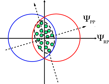
Figure 10: Transverse view of a heavy-ion collision with the reaction plane $\Psi_{\rm RP}$ oriented along the $x$-axis. Indicated are the participants in the overlap region that randomly define a particpant plane $\Psi_{\rm PP}$ for each collision.

Flow fluctuations have become an important part of elliptic flow studies [32, 33, 34, 35, 36, 37, 38, 39, 40, 41, 42]. It is believed that such fluctuations originate mostly from fluctuations in the initial collision geometry. This is illustrated in Fig. 10 which shows participants that are randomly distributed in the overlap region. This collection of participants defines a participant plane $\Psi_{\rm PP}$ [33] which fluctuates, for each event, around the reaction plane $\Psi_{\rm RP}$. These fluctuations can be estimated from calculations in, for instance, a Glauber model.

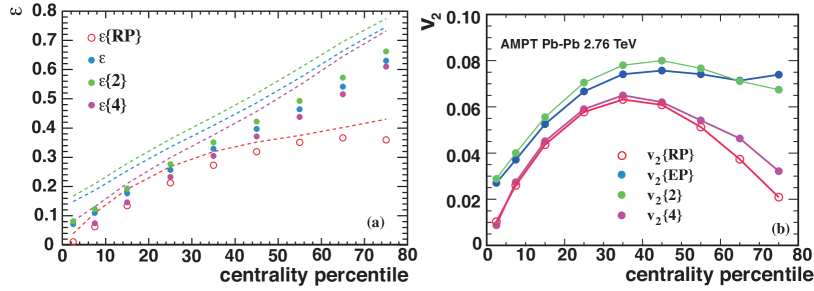
Figure 11: a) The eccentricities from a Glauber calculation for participating nucleons (the solid and open markers) and binary collisions (the dashed lines). b) Various $v_{2}$ estimates compared to the reaction plane value, $v_{2}\{{\rm RP}\}$.

Figure 11a shows the eccentricities (Eq. 5) calculated in a Glauber model. Here $\varepsilon\{{\rm RP}\}$ denotes the eccentricity in the reaction plane, $\varepsilon$ is the participant eccentricity and $\varepsilon\{2\}$ and $\varepsilon\{4\}$ are the participant eccentricities calculated using the cumulants, analogous to the definitions in Eq. 10 [32]. In Fig. 11a the eccentricities are calculated using as a weight the participating nucleons (open and solid markers) or as a weight binary collisions (dashed lines). The figure clearly shows that in both cases $\varepsilon$ is in between $\varepsilon\{2\}$ and $\varepsilon\{4\}$ as is expected from Eq. 11. The figure also shows that $\varepsilon\{4\}$ is close to $\varepsilon\{{\rm RP}\}$ for the $0-40$% centrality range [40, 41]. In Fig. 11b we show a transport model calculation of $v_{2}$ in the AMPT model [43]. In this model the true reaction plane is known so that we can compare the different $v_{2}$ estimates with the value in the reaction plane. The AMPT model uses a Glauber model for the initial conditions and we can therefore compare these estimates with Fig. 11a (the dashed lines). The agreement between $v_{2}\{4\}$ and $v_{2}\{{\rm RP}\}$ holds for most of the centrality range, while for the eccentricities in the Glauber model a large difference is observed for the more peripheral collisions [42].

5 Elliptic Flow Measurements

5.1 The Perfect Liquid

The large elliptic flow observed at RHIC provides compelling evidence for strongly interacting matter which appears to behave like an almost perfect liquid [44, 45]. To quantify the agreement with an almost perfect fluid the significant viscous corrections need to be calculated. Based on different model assumptions the ratio $\eta/s$ has been estimated at $\sqrt{s_{{}_{\rm NN}}}$ = 200 GeV and is found to be below five times the KSS bound [18, 46, 47, 48, 49].

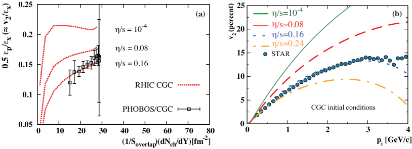
Figure 12: a) The centrality dependence of $v_{2}\{2\}$ compared to viscous hydrodynamic model calculations [24]. b) The transverse momentum dependence of $v_{2}$ compared to the same viscous hydrodynamic calculations [24].

In Fig. 12 we show the centrality and transverse momentum dependence of $v_{2}$ compared to viscous hydrodynamic calculations [24] with different values of $\eta/s$. Using an eccentricity from a CGC inspired calculation, it is seen that both the centrality and transverse momentum dependence is well described with an $\eta/s$ of two times the KSS bound. These calculations are performed under the assumption that the value of $\eta/s$ is constant during the entire evolution. The value used in these calculations should be considered as an effective average of $\eta/s$, because we know from other fluids that $\eta/s$ depends on temperature. In addition, we also know that part of the elliptic flow originates from the hadronic phase. Therefore, knowledge of the temperature dependence and knowledge of the relative contributions from the partonic and hadronic phase is required to quantify $\eta/s$ of the partonic fluid.

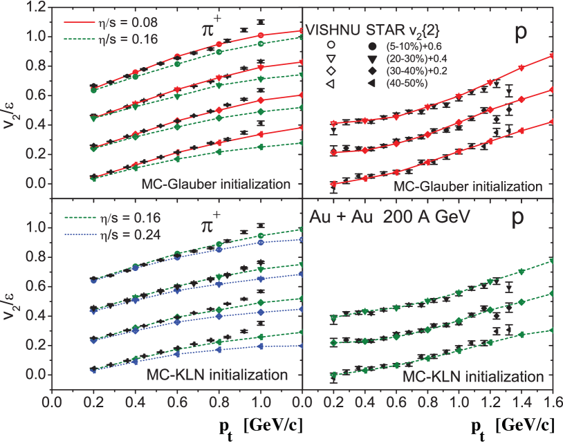
Figure 13: The $v_{2}(\mbox{$p_{\mathrm{t}}$})$ for pions and protons measured by STAR compared to model calculations with different eccentricities and $\eta/s$ [50].

Not only the $v_{2}$ of charged particles but also that of identified particles at RHIC is described in the framework of viscous hydrodynamics at low-$p_{\mathrm{t}}$. Figure 13 shows the measured pion and proton elliptic flow measured by STAR compared to VISHNU [50] model calculations. The VISHNU model is a hybrid model which uses viscous hydrodynamics for the initial stage followed by a hadron cascade afterburner. In the initial viscous hydrodynamic stage $\eta/s$ is temperature independent. The $\eta/s$ magnitude required to describe the pion and proton elliptic flow data are found to be one or two times the KSS bound for a Glauber or CGC eccentricity, respectively. This is in agreement with the magnitude of $\eta/s$ required to describe charged particle $v_{2}$.

While the description of $v_{2}$ measurements is encouraging, it is important to realize that there are still large uncertainties in: (i) the initial eccentricity, (ii) the relative contributions from the hadronic and partonic phase and (iii) the temperature dependence of $\eta/s$. Elliptic flow measurements at the LHC, with a higher center of mass energy, will constrain these uncertainties and will eventually provide a decisive test which of the currently successful model descriptions is the more appropriate.

5.2 Energy Dependence

Lead-Lead collisions at the LHC are expected to produce a system which is hotter and has a longer lived partonic phase than the system created in Au-Au collisions at RHIC energies. As a consequence, the hadronic contribution to the elliptic flow decreases which reduces the uncertainty on the determination of $\eta/s$ in the partonic fluid. Because $\eta/s$ is expected to depend on temperature in both the partonic and hadronic system it was not clear if the elliptic flow would increase or decrease in going from RHIC to LHC energies. Hydrodynamic models [51, 52, 53] and hybrid models [54, 55] that successfully describe flow at RHIC predicted an increase of $\sim$10–30% in $v_{2}$.

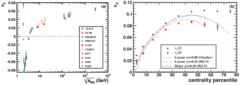
Figure 14: a) Integrated elliptic flow at 2.76 TeV in the 20–30% centrality class compared with results from lower energies taken at similar centralities (From [20]). b) Elliptic flow as a function of event centrality, for the 2- (full circles ) and 4-particle (full squares) cumulant methods compared to viscous hydrodynamic calculations (dashed lines) [20, 56, 57].

Figure 14a shows the measured integrated elliptic flow at the LHC in one centrality bin, compared to results from lower energies. It shows that there is a continuous increase in the elliptic flow from RHIC to LHC energies. In comparison to the elliptic flow measurements in Au–Au collisions at $\mbox{$\sqrt{s_{{}_{\rm NN}}}$}~{}=~{}200$ GeV $v_{2}$ increases by about 30% at $\mbox{$\sqrt{s_{{}_{\rm NN}}}$}~{}=~{}2.76$ TeV.

Figure 14b shows the $v_{2}$ for different centralities measured by ALICE with the two- and four-particle cumulant method. The difference between the two- and four-particle flow estimates for the more central collisions ($<40$%) is expected to be dominated by event-by-event flow fluctuations (see Eq. 11). For the more peripheral collisions the two-particle cumulant is likely biased by non-flow. We already mentioned that $v_{2}\{4\}$ yields estimates of the elliptic flow in the reaction plane which can thus be compared to model predictions of $v_{2}\{{\rm RP}\}$. The curves in Fig. 14b show $v_{2}\{{\rm RP}\}$ from hydrodynamic model calculations for $\mbox{$\sqrt{s_{{}_{\rm NN}}}$}~{}=~{}2.76$ TeV, with initial eccentricities and magnitudes of $\eta/s$ which described the RHIC data. It is seen that in hydrodynamic calculations the observed increase in $v_{2}$ from RHIC to LHC energies is within expectations. Detailed comparisons, however, have to wait till measurements of identified particle spectra and identified particle elliptic flow become available. It will then be important to see if one still obtains a quantitative description of the data in viscous hydrodynamics and what the required magnitude of $\eta/s$ then will be.

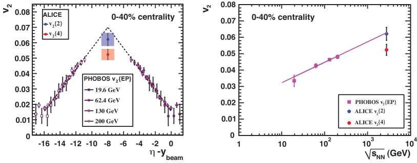
Figure 15: a) Elliptic flow plotted versus $\eta-y_{{\rm beam}}$ for RHIC and the LHC, with for $y_{{\rm beam}}$ the $\mbox{$\sqrt{s_{{}_{\rm NN}}}$}~{}=~{}2.76$ TeV value. The mesh shows the $\eta$-range over which the elliptic flow is constant within statistical uncertainties. b) Elliptic flow versus beam energy. In both figures the uncertainties for ALICE are systematic uncertainties and the $v_{2}$ in 0–40% centrality is obtained by averaging over events instead of over, the more commonly used, particle yield.

In addition to comparisons with detailed dynamic model calculations we might also learn something from what happens to the several simple scaling properties observed at lower energies. For instance, it was shown that the integrated elliptic flow depends linearly on the pseudorapidity $\eta$, measured with respect to the beam rapidity $y_{\rm beam}$ [58], as is shown in Fig. 15a. Based on this scaling behaviour a phenomenological extrapolation [59] from RHIC to the LHC was made (dashed line in Fig. 15a) which predict an increase in $v_{2}$ of $\sim$50%, larger than predictions from most other models. PHOBOS measured $v_{2}$ down to $p_{t}=0$ using the eventplane method which at RHIC is similar to measuring $v_{2}\{2\}$. The measurements at $\eta=0$ for the LHC are below the triangular extrapolation. However, the elliptic flow as function of pseudorapidity measured by ALICE in $|\eta|<0.8$ (mesh in Fig. 15a) is constant within uncertainties. If one takes into account that the $v_{2}(\eta)$ does saturate, like the multiplicity, at each energy around midrapidity then the longitudinal scaling might hold up to LHC energies.

Figure 15b shows that the energy dependence of elliptic flow at midrapidity also seems to follow a rather simple scaling: the measured elliptic flow for four beam energies at RHIC shows a linear increase, extrapolating this to $\mbox{$\sqrt{s_{{}_{\rm NN}}}$}~{}=~{}2.76$ TeV results in a $v_{2}$ which agrees well with the ALICE measurement.

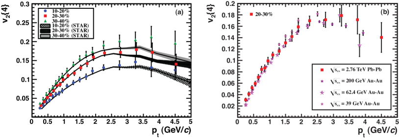
Figure 16: a) $v_{2}${4}($p_{\mathrm{t}}$) for various centralities compared to STAR measurements. The data points in the 20–30% centrality bin are shifted in $p_{\rm t}$ for visibility. b) $v_{2}${4}($p_{\mathrm{t}}$) for a collision energy range which covers almost two orders of magnitude [60]

The observed increase in the elliptic flow as function of beam energy is either due to an increase in $p_{\mathrm{t}}$-differential flow or due to an increase in the average transverse momentum of the charged particles. In most hydrodynamic model calculations the $p_{\mathrm{t}}$-differential elliptic flow of charged particles does not change significantly [51, 52], while the radial (azimuthally symmetric) flow does increase which leads to an increase in the average transverse momentum. The larger radial flow also leads to a decrease of the elliptic flow at low transverse momentum, which is most pronounced for heavy particles. Figure 16a compares the $p_{\mathrm{t}}$-differential elliptic flow of charged particles for three centralities at the LHC with STAR measurements at RHIC. It is seen that the $p_{\mathrm{t}}$-differential elliptic flow is the same within experimental uncertainties. In Fig. 16b the $p_{\mathrm{t}}$-differential elliptic flow measured at four beam energies is shown. The agreement of $v_{2}(\mbox{$p_{\mathrm{t}}$})$ at these beam energies, which differ by almost two orders of magnitude, is remarkable. Measurements of identified particle elliptic flow at these energies will reveal if this agreement can be understood in hydrodynamic model calculations.

6 Summary

In this review, I have shown that elliptic flow is one of the most informative observables in heavy-ion collisions. Nevertheless, the wealth of experimental information obtained from elliptic flow is far from being fully explored. The theoretical understanding of the experimental data is rapidly improving as is our understanding of the dynamics in heavy-ion collisions and the properties of the new state of matter, the quark gluon plasma. New high quality data from the LHC recently became available which shows that at LHC energies elliptic flow can be studied with unprecedented precision. This is because of the increase in particle multiplicity and also because of the increase in the flow signal itself. Due to the expected longer life time of the quark gluon plasma and the smaller contributions from the hadronic phase it is argued that the LHC is also better suited to determine $\eta/s$ of the partonic fluid [61]. Measurements of identified particle elliptic flow at the LHC and in particular the stronger mass dependence (splitting) of $v_{2}(\mbox{$p_{\mathrm{t}}$})$ will be important to confirm the current theoretical picture. Additional constraints on $\eta/s$ can be obtained by measurements of the other anisotropic flow harmonics $v_{3}$, $v_{4}$ and $v_{5}$. In the near future these measurements will become available and significantly increase our understanding of ultra-relativistic nuclear collisions and multi-particle production in general.

References

- [1] Peter W. Higgs. Phys. Lett. 12:132–133, 1964.
- [2] Peter W. Higgs. Phys. Rev. Lett. 13:508–509, 1964.
- [3] F. Englert and R. Brout. Phys. Rev. Lett. 13:321–322, 1964.
- [4] Yoichiro Nambu and G. Jona-Lasinio. Phys. Rev. 122:345–358, 1961.
- [5] D. J. Gross and Frank Wilczek. Phys. Rev. D8:3633–3652, 1973.
- [6] H. David Politzer. Phys. Rev. Lett. 30:1346–1349, 1973.
- [7] Edward V. Shuryak. Phys. Rept. 61:71–158, 1980.
- [8] A. Bazavov, T. Bhattacharya, M. Cheng et al., Phys. Rev. D80, 014504 (2009).
- [9] G. F. Chapline, M. H. Johnson, E. Teller, and M. S. Weiss. Phys. Rev. D8:4302–4308, 1973.
- [10] T. D. Lee and G. C. Wick. Phys. Rev. D9:2291, 1974.
- [11] T. D. Lee. Phys. Rev. D19:1802, 1979.
- [12] John C. Collins and M. J. Perry. Phys. Rev. Lett. 34:1353, 1975.
- [13] Robert D. Pisarski and Frank Wilczek. Phys. Rev. D29:338–341, 1984.
- [14] J. Y. Ollitrault, Phys. Rev. D 46, 229 (1992).
- [15] S. A. Voloshin, A. M. Poskanzer and R. Snellings, in Landolt-Boernstein, Relativistic Heavy Ion Physics, Vol. 1/23 (Springer-Verlag, 2010), p 5-54. arXiv:0809.2949 [nucl-ex].
- [16] U. W. Heinz, arXiv:0901.4355 [nucl-th].
- [17] P. Huovinen and P. V. Ruuskanen, Ann. Rev. Nucl. Part. Sci. 56, 163 (2006)
- [18] D. A. Teaney, arXiv:0905.2433 [nucl-th].
- [19] M. L. Miller, K. Reygers, S. J. Sanders et al., Ann. Rev. Nucl. Part. Sci. 57, 205-243 (2007).
- [20] K. Aamodt et al. [The ALICE Collaboration], Phys. Rev. Lett. 105, 252302 (2010).
- [21] P. F. Kolb, U. W. Heinz, In *Hwa, R.C. (ed.) et al.: Quark gluon plasma* 634-714.
- [22] P. Huovinen, P. Petreczky, Nucl. Phys. A837, 26-53 (2010).
- [23] D. Teaney, Phys. Rev. C68, 034913 (2003).
- [24] M. Luzum, P. Romatschke, Phys. Rev. C78, 034915 (2008).
- [25] P. Kovtun, D. T. Son, A. O. Starinets, Phys. Rev. Lett. 94, 111601 (2005).
- [26] L. P. Csernai, J. .I. Kapusta, L. D. McLerran, Phys. Rev. Lett. 97, 152303 (2006).
- [27] R. A. Lacey, N. N. Ajitanand, J. M. Alexander et al., Phys. Rev. Lett. 98, 092301 (2007).
- [28] T. Hirano, U. W. Heinz, D. Kharzeev et al., J. Phys. G G34, S879-882 (2007).
- [29] N. Borghini, P. M. Dinh, J. -Y. Ollitrault, Phys. Rev. C64, 054901 (2001).
- [30] C. Adler et al. [ STAR Collaboration ], Phys. Rev. C66, 034904 (2002).
- [31] A. Bilandzic, R. Snellings and S. Voloshin, arXiv:1010.0233 [nucl-ex], submitted to PRC
- [32] M. Miller and R. Snellings, arXiv:nucl-ex/0312008.
- [33] S. Manly et al. [PHOBOS Collaboration], Nucl. Phys. A 774, 523 (2006).
- [34] P. Sorensen, [arXiv:0905.0174 [nucl-ex]].
- [35] G. -Y. Qin, H. Petersen, S. A. Bass et al., Phys. Rev. C82, 064903 (2010).
- [36] R. A. Lacey, R. Wei, N. N. Ajitanand et al., [arXiv:1009.5230 [nucl-ex]].
- [37] T. Hirano, Y. Nara, Nucl. Phys. A830, 191C-194C (2009).
- [38] J. -Y. Ollitrault, A. M. Poskanzer, S. A. Voloshin, Phys. Rev. C80, 014904 (2009).
- [39] S. Mrowczynski, Acta Phys. Polon. B40, 1053-1074 (2009).
- [40] R. S. Bhalerao, J. -Y. Ollitrault, Phys. Lett. B641, 260-264 (2006).
- [41] S. A. Voloshin, A. M. Poskanzer, A. Tang et al., Phys. Lett. B659, 537-541 (2008).
- [42] B. Alver, B. B. Back, M. D. Baker et al., Phys. Rev. C77, 014906 (2008).
- [43] Z. -W. Lin, C. M. Ko, B. -A. Li et al., Phys. Rev. C72, 064901 (2005).
- [44] I. Arsene et al., Nucl. Phys. A757, 1 (2005); B. B. Back et al., ibid., p. 28; J. Adams et al., ibid., p. 102; K. Adcox et al., ibid., p. 184.
- [45] M. Gyulassy, L. McLerran, Nucl. Phys. A 750, 30 (2005).
- [46] C. Shen, U. Heinz, P. Huovinen et al., Phys. Rev. C82, 054904 (2010).
- [47] H. Song, S. A. Bass, U. W. Heinz et al., [arXiv:1011.2783 [nucl-th]].
- [48] H. Masui, J-Y. Ollitrault, R. Snellings et al., Nucl. Phys. A830, 463C-466C (2009).
- [49] J. L. Nagle, P. Steinberg, W. A. Zajc, Phys. Rev. C81, 024901 (2010).
- [50] H. Song, S.A Bass, U.W Heinz et al., [arXiv:1101.4638 [nucl-th]].
- [51] H. Niemi, K. J. Eskola and P. V. Ruuskanen, Phys. Rev. C 79, 024903 (2009)
- [52] G. Kestin and U. W. Heinz, Eur. Phys. J. C 61, 545 (2009)
- [53] M. Luzum and P. Romatschke, Phys. Rev. Lett. 103, 262302 (2009)
- [54] T. Hirano, P. Huovinen and Y. Nara, arXiv:1010.6222 [nucl-th].
- [55] T. Hirano, U. W. Heinz, D. Kharzeev, R. Lacey and Y. Nara, Phys. Lett. B 636, 299 (2006)
- [56] M. Luzum, [arXiv:1011.5173 [nucl-th]].
- [57] U. Heinz and C. Shen, private communication.
- [58] B. B. Back et al. [ PHOBOS Collaboration ], Phys. Rev. Lett. 94, 122303 (2005).
- [59] W. Busza, J. Phys. G 35, 044040 (2008)
- [60] L. Kumar, f. t. S. Collaboration, [arXiv:1101.4310 [nucl-ex]].
- [61] H. Niemi, G. S. Denicol, P. Huovinen et al., [arXiv:1101.2442 [nucl-th]].