Extremely Correlated Fermi Liquids

Abstract

We present the theory of an extremely correlated Fermi liquid with $U\to\infty$. This liquid has an underlying auxiliary Fermi liquid Greens function that is further caparisoned by extreme correlations. The theory leads to two parallel hierarchies of equations that permit iterative approximations in a certain parameter. Preliminary results for the spectral functions display a broad background and a distinct $T$ dependent left skew. An important energy scale $\Delta(\vec{k},x)$ emerges as the average inelasticity of the FL Greens function, and influences the photoemission spectra profoundly. A duality is identified wherein a loss of coherence of the ECFL results from an excessively sharp FL.

Introduction Correlated electron systems attract two distinct approaches. An intermediate to strong coupling approach is used when the interaction $U$ is comparable to the band width $2W$, and has seen some success in recent timesdmft . On the other hand, Andersonanderson has argued that myriad experiments on high $T_{c}$ superconductors require a better understanding of the  $t$-$J$  model physics. This model sets $U\to\infty$ right away i.e. leads to extreme correlations and involves Gutzwiller projected Fermi operators that are non canonical. Thus Wick’s theorem is immediately lost, and perturbative schemes encoding the Feynman Dyson approach become useless. Since this approach is at the root of most current many body physics text books, the task of understanding the  $t$-$J$  model is not lightly undertaken.

The Schwinger approach to interacting field theories is a powerful and attractive alternative. It is fundamentally non perturbative, where Wick’s theorem is bypassed by dealing with suitable inverse Greens functions. Conventional many body theory for canonical Fermions can also be cast into this approach, and leads to the standard results. In Ref. ECQL, (henceforth I), the author has recently applied the Schwinger method to the  $t$-$J$  model, and found a class of solutions that are termed as extremely correlated quantum liquids. That state is presumably realized under suitable conditions. However it gives a Fermi surface (FS) volume that is always distinct from that of the Fermi gas. This is contrast to the case of Fermi liquids (FL), where the important theorem of Luttinger and Ward (L-W) luttinger ; agd mandates the invariance of the FS volume under interactions.

In this paper we propose a state of matter termed as an extremely correlated Fermi liquid (ECFL). The ECFL found here, represents an alternate class of solutions for the  $t$-$J$  model, where the Fermi surface satisfies the Fermi gas (i.e. L-W) volume. In this work we present the essentials of the formalism, and display preliminary results on spectral functions that are suggestive of the relevance of the ECFL state to cuprate materials. An inherent flexibility of the Schwinger approach permits the construction of an alternate class of solutions from the one found in I. The excitations of the ECFL state may be thought of as bare electrons undergoing a double layer of renormalization: the FL dressing into quasiparticles that are further caparisoned (i.e. decorated) by extreme correlations.

Formalism: The physical projected electronic Greens function ${\cal{G}}$ satisfies an equation of motion (EOM) (I-29) written compactly in matrix form as

$$(\partial_{\tau_{i}}-{\bm{\mu}}){\cal{G}}(i,f)=-\delta(i,f)\left\{1-\gamma(i)\right\}-{\cal V}_{i}\cdot{\cal{G}}(i,f)$$

$$-X(i,{\bar{\mathbf{j}}})\cdot{\cal{G}}({\bar{\mathbf{j}}},f)-Y(i,{\bar{\mathbf{j}}})\cdot{\cal{G}}({\bar{\mathbf{j}}},f),$$ (1)

where ${\bm{\mu}}$ is the chemical potential and an implicit integration over space time variables such as ${\bar{\mathbf{j}}}$, written with bold overlined letters, is implied,

$$X(i,j) = -t(i,j)\ (D(i)+D(j))+\frac{1}{2}J(i,{\bar{\mathbf{k}}})\ (D(i)+D({\bar{\mathbf{k}}}))\delta(i,j)$$

$$Y(i,j) = -t(i,j)\ (\mathds{1}-\gamma(i)-\gamma(j))+\frac{1}{2}J(i,{\bar{\mathbf{k}}})\ (\mathds{1}-\gamma(i)-\gamma({\bar{\mathbf{k}}}))\delta(i,j).$$ (2)

In the above expressionfootnote-sym , we used $\gamma({i})={\cal{G}}^{k}(i,i)$ with the $k$ conjugation defined by $(M^{k})_{\sigma_{1}\sigma_{2}}=M_{\bar{\sigma}_{2}\bar{\sigma}_{1}}\sigma_{1}\sigma_{2}$, and $D_{\sigma_{1}\sigma_{2}}(i)=\sigma_{1}\sigma_{2}\frac{\delta}{\delta{\cal V}_{i}^{\bar{\sigma}_{1}\bar{\sigma}_{2}}}$ . The added (Bosonic) source term ${\cal V}_{i}^{\sigma_{1}\sigma_{2}}(\tau_{i})$ is central to this approach; it is a space-time dependent field that couples to the charge and spin densities through a term in the action: $\sum_{i\sigma}\int_{0}^{\beta}d\tau\ {\cal V}_{i}^{\sigma_{1}\sigma_{2}}(\tau)\ X^{\sigma_{1}\sigma_{2}}_{i}(\tau)$, where $X_{i}^{\sigma_{1}\sigma_{2}}$ is the spin and density operator at site $i$ that acts as $|\sigma_{1}\rangle\langle\sigma_{2}|$ .

An important technical problem highlighted in I  is to deal with the time dependence of the $\gamma(i)$ term in Eq. (1) which makes the theory non canonical. Here we use the decomposition into two factors fn1 :

$${\cal{G}}(a,b) = {\bf g}(a,{\bar{\mathbf{b}}})\cdot\mu({\bar{\mathbf{b}}},b),$$ (3)

and express $\gamma(i)=({\bf g}(i,{\bar{\mathbf{j}}})\cdot\mu({\bar{\mathbf{j}}},i))^{k}$. The object ${\bf g}$ is an auxiliary FL Greens function and $\mu({\bar{\mathbf{b}}},b)$ is an appurtenant (or supplementary) factor that is determined below. Antiperiodic boundary conditions ${\cal{G}}(0,\tau_{f})=-{\cal{G}}(\beta,\tau_{f})$ and ${\cal{G}}(\tau_{i},0)=-{\cal{G}}(\tau_{i},\beta)$ imply that both factors ${\bf g}$ and $\mu$ are Fourier transformed using Fermionic Matsubara frequencies. We define the inverse Greens function ${\bf g}^{-1}(a,{\bar{\mathbf{b}}})\cdot{\bf g}({\bar{\mathbf{b}}},b)=\mathds{1}\delta(a,b)$, and thence a vertex function $\Lambda^{\sigma_{1}\sigma_{2}}_{\sigma_{3}\sigma_{4}}(p,q;r)=-\frac{\delta}{\delta{\cal V}^{\sigma_{3}\sigma_{4}}_{r}}\ \{{\bf g}^{-1}_{\sigma_{1}\sigma_{2}}(p,q)\ \}.$ Thus ${\bf g}$, $\mu$ and ${\bf g}^{-1}$ are matrices in the spin space, and the vertex $\Lambda$ has four indices. We also define a linear operator

$${\bf L}(i,f)=\left(t(i,{\bar{\mathbf{j}}})\ \xi^{*}\cdot{\bf g}({\bar{\mathbf{j}}},f)-\frac{1}{2}J(i,{\bar{\mathbf{j}}})\ \xi^{*}\cdot{\bf g}(i,f)\right)\cdot\left(\frac{\delta}{\delta{\cal V}_{i}^{*}}+\frac{\delta}{\delta{\cal V}_{\bar{\mathbf{j}}}^{*}}\right),$$ (4)

where the matrix $\xi^{*}_{\sigma_{1}\sigma_{2}}=\sigma_{1}\sigma_{2}$. The ^∗ is used as a place holder that transmits the spin indices (after conjugation) of the $\xi$ matrix to the source matrix ${\cal V}$ in the functional derivative. This notation used is illustrated in component form by $\cdots\xi^{*}_{\sigma_{a}\sigma_{b}}\cdots{\delta}/{\delta{\cal V}_{\bar{\mathbf{j}}}^{*}}=\cdots\sigma_{a}\sigma_{b}\cdots\delta/{\delta{\cal V}_{\bar{\mathbf{j}}}^{\bar{\sigma}_{a},\bar{\sigma}_{b}}}.$

A useful chain rule for the functional derivative is noted

$$D(r)\cdot{\cal{G}}(a,b) = \xi^{*}\cdot{\bf g}(a,{\bar{\mathbf{c}}})\cdot\ \Lambda_{*}({\bar{\mathbf{c}}},{\bar{\mathbf{d}}};r)\ \cdot{\cal{G}}({\bar{\mathbf{d}}},b)$$ (5)

$$+\xi^{*}\cdot{\bf g}(a,{\bar{\mathbf{b}}})\cdot\ \left(\frac{\delta}{\delta{\cal V}^{*}_{r}}\mu({\bar{\mathbf{b}}},{b})\right)$$

Using this chain rule, we see that

$$X(i,{\bar{\mathbf{j}}})\cdot{\cal{G}}({\bar{\mathbf{j}}},f) \equiv \Phi(i,{\bar{\mathbf{b}}})\cdot{\cal{G}}({\bar{\mathbf{b}}},f)+\Psi(i,f)$$ (6)

where

$$\Phi(i,m)={\bf L}(i,{\bar{\mathbf{i}}})\cdot{\bf g}^{-1}({\bar{\mathbf{i}}},m)$$

$$\Psi(i,m)=-\ {\bf L}(i,{\bar{\mathbf{i}}})\cdot\mu({\bar{\mathbf{i}}},m)$$ (7)

Thus the two fundamental functions of this formalism $\Phi,\Psi$ are closely connected as they arise from applying the same operator to the two factors of ${\cal{G}}$. Defining $Y_{0}(i,j)=\left(-t(i,j)+\frac{1}{2}J(i,{\bar{\mathbf{k}}})\ \delta(i,j)\right)\mathds{1}$, and $Y_{1}(i,j)=t(i,j)\ (\gamma(i)+\gamma(j))-\frac{1}{2}\ \delta(i,j)\ J(i,{\bar{\mathbf{k}}})\ (\gamma(i)+\gamma({\bar{\mathbf{k}}}))$, also denote the Fermi gas Greens function

$${\bf g}^{-1}_{0}(i,f)=\{-(\partial_{\tau_{i}}-{\bm{\mu}})\mathds{1}-{\cal V}_{i})\delta(i,f)-\ Y_{0}(i,f)\}.$$ (8)

Collecting everything, the exact EOM can now be written neatly as

$$\{{\bf g}^{-1}_{0}(i,{\bar{\mathbf{j}}})-\lambda\ Y_{1}(i,{\bar{\mathbf{j}}})-\lambda\ \Phi(i,{\bar{\mathbf{j}}})\}\ \cdot{\bf g}({\bar{\mathbf{j}}},{\bar{\mathbf{f}}})\cdot\mu({\bar{\mathbf{f}}},f)$$

$$=\delta(i,f)\left(\mathds{1}-\lambda\ \gamma(i)\right)+\lambda\ \Psi(i,f).$$ (9)

We have introduced the parameter $\lambda$ above, with $0\leq\lambda\leq 1$, in order to provide an adiabatic path between the Fermi gas at $\lambda=0$ and the ECFL at $\lambda=1$, and also an iterative scheme in powers of $\lambda$ connecting the two endpoints.

We now choose the hitherto undetermined function $\mu$ as:

$$\mu(i,f)=\delta(i,f)\left(\mathds{1}-\lambda\ \gamma(i)\right)+\lambda\ \Psi(i,f),$$ (10)

so that Eq. (9) reduces to a canonical FL type equation:

$$\{{\bf g}^{-1}_{0}(i,{\bar{\mathbf{j}}})-\lambda\ Y_{1}(i,{\bar{\mathbf{j}}})-\lambda\ \Phi(i,{\bar{\mathbf{j}}})\}\ \cdot{\bf g}({\bar{\mathbf{j}}},f)=\delta(i,f).$$ (11)

Notice that the right hand side has a pure $\delta$ function as in a canonical Fermi liquid type theory. To summarize, the EOM Eq. (1) under the decomposition Eq. (3) leads to Eq. (9). In turn this splits exactly into two coupled sets of equations Eq. (7), Eq. (10) and Eq. (11) for the two factors ${\bf g}$ and $\mu$. Note that the entire procedure is exact, we write explicit forms of these equations below and then introduce approximate methods to solve them .

Inverting we find Dyson’s equation for the auxiliary FL Greens function:

$${\bf g}^{-1}(i,m)=\{{\bf g}^{-1}_{0}(i,m)-\lambda\ Y_{1}(i,m)-\lambda\ \Phi(i,m)\}.$$ (12)

Taking functional derivatives of Eq. (10) and Eq. (12) w.r.t. ${\cal V}$, and comparing with Eq. (4) and Eq. (7) we generate two parallel hierarchies of equations for ${\bf g}$ and $\mu$ that form the core of this formalism. The hierarchy for ${\bf g}$ is essentially autonomous and drives that for $\mu$. Starting with the Fermi gas at $O(\lambda^{0})$, an iterative process similar to the skeleton graph expansion of L-Wluttinger can be built up, such that terms of $O(\lambda^{n})$ arise from differentiating lower order terms of $O(\lambda^{n-1})$. Systematic approximations may thus be arranged to include all terms of $O(\lambda^{n})$ for various $n$lambda . The number of particles is given by $\frac{1}{2}n(i)={\bf g}(i,{\bar{\mathbf{i}}})\cdot\mu({\bar{\mathbf{i}}},i),$ and with

$${\cal U}^{\sigma_{1}\sigma_{2}}_{\sigma_{3}\sigma_{4}}(a,b;c)\equiv\frac{\delta\mu_{\sigma_{1}\sigma_{2}}(a,b)}{\delta{\cal V}_{c}^{\sigma_{3}\sigma_{4}}},$$ (13)

the equations to solve simultaneously are Eq. (7), Eq. (12) and Eq. (10). The density and spin density response functions (I-F1,I-F-7) can be found from differentiating ${\cal{G}}$ i.e. $\Upsilon^{\sigma_{1}\sigma_{2}}_{\sigma_{3}\sigma_{4}}(p,q;r)=\frac{\delta}{\delta{\cal V}_{c}^{\sigma_{3}\sigma_{4}}}\ \left\{{\cal{G}}_{\sigma_{1}\sigma_{2}}(p,q)\right\}.$

Zero source limit in Fourier space: When we turn off the source ${\cal V}$, the various matrix function ${\cal{G}},{\bf g},\mu$ become spin diagonal and translation invariant so we can Fourier transform these conveniently. We note the basic result expressing ${\cal{G}}$ as a simple product of two functions in $k$ space:

$${\cal{G}}(k) = \ {\bf g}(k)\ {\mu(k)},\;\;\;\mu(k)=1-\lambda\ \frac{n}{2}+\lambda\ \Psi(k)$$

$${\bf g}^{-1}(k) = i\omega_{k}+{\bm{\mu}}-\varepsilon_{k}(1-\lambda\ n)-\lambda\ \Phi(k)$$ (14)

where $\varepsilon_{k}$ is the Fourier transform of the hopping matrix $-t(i,j)$, and an uninteresting constant term is absorbed in ${\bm{\mu}}$ here and below.

Here ${\bf g}$ plays the role of an underlying auxiliary FL with a self energy $\Phi$, and $\Psi$ acts as an extra spectral weight that vanishes at high frequency, leaving the exact weight $1-\frac{n}{2}$ valid for a projected electron (as in I) for $\lambda=1$. Denoting $\sum_{k}\to\frac{1}{N_{s}\ \beta}\sum_{i\omega_{k},\vec{k}}$ with $N_{s}$ sites, the particle number sum rule is $\sum_{k}\mu(k){\bf g}(k)=\frac{n}{2}$, i.e.

$$\frac{n}{2}=\sum_{k}{\bf g}(k)+\lambda\sum_{k}(\Psi(k)-\frac{n}{2})\ {\bf g}(k).$$ (15)

In this formalism, at $k\sim k_{F},\ x=0$ that is relevant to the L-W sum rule, the $\Re e\ {\bf g}(k)$ dominates $\Re e\ {\cal{G}}(\vec{k},0)$ (since $\Re e\ \Psi(\vec{k},0)$ is smooth through the FS). Requiring consistency with the L-W theorem forces us to pin any sign change of $\Re e\ {\bf g}(\vec{k},0)$ to the free case, whereby we impose a second level sum rule

$$\sum_{k}\Psi(k)\ {\bf g}(k)=\frac{n^{2}}{4},\;\;\mbox{and}\;\;\sum_{k}{\bf g}(k)=\frac{n}{2}.$$ (16)

This can be viewed as a splitting of the usual number sum rule Eq. (15) fn2 . With $E(p_{1},p_{2})=\left(\varepsilon_{p_{1}}+\varepsilon_{p_{2}}+\frac{1}{2}\hat{J}(0)+\frac{1}{2}\hat{J}(p_{1}-p_{2})\right)$ we find

$$\Phi(k) = \ \sum_{p}\ E(k,p)\ {\bf g}(p)\ \Lambda^{(a)}(p,k)$$

$$\Psi(k) = \ \sum_{p}\ E(k,p)\ {\bf g}(p)\ {\cal U}^{(a)}(p,k)$$ (17)

and the spin labels are from I  with the usual significance $\Lambda^{(a)}=\Lambda^{(2)}-\Lambda^{(3)}=\frac{1}{2}\Lambda^{(s)}-\frac{3}{2}\Lambda^{(t)}$.

Next we introduce the spectral representation of various functions $Q$ that vanish at infinity: $Q(i\omega_{Q})=\int_{-\infty}^{\infty}\ dx\ \frac{\rho_{Q}(x)}{i\omega_{Q}-x}$ and $\rho_{Q}(x)=-\frac{1}{\pi}\ \Im m\ Q(x+i0^{+}),$ with $x^{+}\equiv x+i0^{+}$. The Matsubara frequency $\omega_{Q}$ is Fermionic (Bosonic) if $Q$ is Fermionic (Bosonic). Proceeding further, at any order in $\lambda$, the two hierarchies give us coupled equations for the spectral densities of the physical particles $\rho_{{\cal{G}}}(\vec{k},x)$ as well as the underlying Fermi liquid $\rho_{{\bf g}}(\vec{k},x)$, in terms of the two objects $\rho_{\bar{\Phi}}(\vec{k},x)$ and $\rho_{\Psi}(\vec{k},x)$ and their Hilbert transforms. The Lehmann representation implies that $\rho_{{\cal{G}}}(\vec{k},x)$ is positive at all $\vec{k},x$. In making approximations, this important and challenging constraint must be kept in mind.

Solution of ${\bf g}^{-1}$ and $\mu$ to order $O(\lambda)^{2}$: We next discuss a systematic expansion in powers of $\lambda$ lambda , obtained by taking functional derivatives of Eq. (10) and Eq. (12) to generate expressions for the vertices given the Greens functions via $\Lambda\sim-\frac{\delta}{\delta{\cal V}}{\bf g}^{-1}$ and ${\cal U}\sim\frac{\delta}{\delta{\cal V}}\mu$. To lowest order in $\lambda$ , the bare vertex $\Lambda^{(a)}=-1$, this term is absorbed in a renormalization of the band dispersion to $\overline{\varepsilon}_{k}$ in Eq. (14) dispersion-renorm , and the remaining term denoted by $\bar{\Phi}(k)$. To this order ${\cal U}^{(a)}=0$. Proceeding to the next non trivial order in $\lambda$, by taking the functional derivative of Eq. (10) and Eq. (12) we find after a brief calculation:

$$\Psi(k) = -2\lambda\ \sum_{p,q}\ E(k,p)\ {\bf g}(p)\ {\bf g}(q)\ {\bf g}(q+p-k)$$

$$\bar{\Phi}(k) = -2\lambda\ \sum_{p,q}\ E(k,p)\left(E(p,k)+E(q+p-k,p)\right)$$ (18)

$${\bf g}(p)\ {\bf g}(q)\ {\bf g}(q+p-k).$$

From Eq. (14) we note that these expressions Eq. (18) lead to a calculation of ${\bf g}^{-1}$ and $\mu$ correct upto $O(\lambda^{2})$. Frequency dependent corrections arise only to second order in $\lambda$, which is analogous to the structure of the canonical many body theory within the skeleton graph expansion. We may now set $\lambda=1$ and study the resulting theory as the first step in exploring this formalism.

Denote $f(x)=\frac{1}{(\exp{\beta x})+1}$ as the Fermi distribution functions and $\bar{f}(x)=1-f(x)$ , and denote the usual Fermi factors from second order theory

$${\cal W}=\left\{f(u)f(w)\bar{f}(v)+f(v)\bar{f}(u)\bar{f}(w)\right\}\delta(u+w-v-x),$$

a function of the frequencies $u,v,w,x$, and

$${\cal Y}=\ \int_{u,v,w}{\cal W}\ \rho_{{\bf g}}(\vec{q},w)\rho_{{\bf g}}(\vec{p},u)\rho_{{\bf g}}(\vec{q}+\vec{p}-\vec{k},v),$$ (19)

a function of $\vec{k},\vec{p},\vec{q}$ and $x$. We may then write the spectral functions corresponding to Eq. (18)

$$\rho_{\bar{\Phi}}(\vec{k},x) = 2\sum_{\vec{p},\vec{q}}E(\vec{k},\vec{p})\left(E(\vec{p},\vec{k})+E(\vec{q}+\vec{p}-\vec{k},\vec{p})\right){\cal Y}$$

$$\rho_{\Psi}(\vec{k},x) = 2\ \sum_{\vec{p},\vec{q}}\ E(\vec{k},\vec{p})\ {\cal Y}.$$ (20)

The functions appearing in Eq. (20) are familiar from Fermi liquidsagd ; luttinger , and encode the usual phase space constraints of that theory. This leads to the low temperatures behaviour $\sim\mbox{max}\left\{x^{2},(\pi k_{B}T)^{2}\right\}$, for both objects $\Im m\ \Psi(k,x,T)$ and $\Im m\ \bar{\Phi}(k,x,T)$. The real parts of these objects are smooth through the Fermi surface, as one expects from the real part of the self energy in a FL, and hence motivates the second level sum rule Eq. (16).

From Eq. (14) we write the exact expression for the physical spectral function $\rho_{{\cal{G}}}$:

$$\rho_{{\cal{G}}}(\vec{k},x)=\rho_{{\bf g}}(\vec{k},x)\left(\left\{1-\frac{n}{2}\right\}\ +\frac{\xi_{k}-x}{\Delta(\vec{k},x)}+\eta(\vec{k},x)\right),$$ (21)

where $\xi_{k}=\hat{\varepsilon}_{k}-{\bm{\mu}}$, and the important energy scale $\Delta(\vec{k},x)$ and the term $\eta$ is defined as:

$$\Delta(\vec{k},x) = -\frac{\rho_{\bar{\Phi}}(\vec{k},x)}{\rho_{\Psi}(\vec{k},x)},$$ (22)

$$\eta(\vec{k},x) = \Re e\Psi(\vec{k},x^{+})+\frac{1}{\Delta(\vec{k},x)}\Re e\Phi(\vec{k},x^{+}).~{}$$ (23)

The sign of the energy scale $\Delta$ in Eq. (22) is expected to be positive from Eq. (20). The dimensionless term $\eta$ augments the spectral weight at the Fermi level. The equations necessary to solve the theory to $O(\lambda^{2})$ may be summarized as Eq. (14), Eq. (16), Eq. (18) and Ref. (dispersion-renorm, ) giving rise to the spectral function Eq. (21). These require further numerical work that is underway, it leads to spectral functions in 2 and 3 dimensions that will be published separately. However it also provides a very interesting insight about the theory in high dimensions that is pursued analytically next.

Solution in high dimensions: In sufficiently high dimensions, we show next that the dimensionless term $\eta$ vanishes identically leading to a great simplification. For sufficiently high dimensions we can ignore the momentum dependence of ${\cal Y}$ in Eq. (19) and assume $\rho_{\Phi}(\vec{k},x)\sim C_{\Phi}\ \sigma(x)$, and $\rho_{\bar{\Psi}}(\vec{k},x)\sim C_{\Psi}\ \sigma(x)$, as functions of frequency only. Here $\sigma(x)$ extends over energy range $\omega_{c}\sim O(2W)$, and $C_{\Phi}$ has dimensions of inverse energy and is positive due to $\rho_{\bar{\Phi}}$. Its Hilbert transform is called $h(x)\equiv{\cal P}\ \int\ dy\ \frac{\sigma(y)}{x-y}$. We use an analytically tractable Fermi liquid modelfn6 with $\tau=\pi k_{B}T$, where we set:

$$\sigma(x)=\ \{x^{2}+\tau^{2}\}e^{-C_{\Phi}\{x^{2}+\tau^{2}\}/\omega_{c}}\ .$$ (24)

The peak value of $C_{\Phi}\ \sigma(x)$ is of $O(1)$ and independent of $C_{\Phi}$ fn3 . The other constant $C_{\Psi}$ is dimensionless and negative. To complete the model, we note that the real parts are given in terms of $h(x)$ as $\Re e\ \bar{\Phi}(x^{+})=C_{\Phi}\ h(x)$ and $\Re e{\Psi}(x^{+})=C_{\Psi}\ h(x)$. With this choice the auxiliary spectral weight $\eta(k,x)$ vanishes identically in Eq. (23). With $\Gamma(x)\equiv\pi C_{\Phi}\ \sigma(x)$ and $\epsilon(\xi,x)\equiv\left(x-\xi-C_{\Phi}\ h(x)\right)$ we may write $\rho_{{\bf g}}(\xi,x)=\frac{1}{\pi}\frac{\Gamma(x)}{\Gamma^{2}(x)+\epsilon^{2}(\xi,x)}$ and $\Re e\ {\bf g}(\xi,x)=\frac{\epsilon(\xi,x)}{\Gamma^{2}(x)+\epsilon^{2}(\xi,x)}$. Denoting $\langle Q(\xi)\rangle_{\xi}=\int\ d\xi\ N_{B}(\xi)Q(\xi)$, where $N_{B}(\xi)$ is the band density of states per spin, the chemical potential is fixed using $\frac{n}{2}=\int_{-\infty}^{\infty}\ dx\ f(x)\langle\rho_{{\bf g}}(\xi,x)\rangle_{\xi}$.

The energy parameter $\Delta(\vec{k},x)$ in Eq. (22) is a constant. We scale out a factor to define

$$\Delta_{o}=\frac{n^{2}}{4}\Delta(\vec{k},x)=-\frac{n^{2}}{4}\ \frac{C_{\Phi}}{C_{\Psi}}.$$ (25)

The physically observable electronic spectral function reads

$$\rho_{{\cal{G}}}(\xi,x)=\frac{\Gamma(x)}{\pi}\frac{\left(\left\{1-\frac{n}{2}\right\}+\left(\frac{n^{2}}{4}\right)\left\{\frac{\xi-x}{\Delta_{0}}\right\}\right)_{+}}{\Gamma^{2}(x)+\epsilon^{2}(\xi,x)}.$$ (26)

Here the condition $(f)_{+}\equiv\mbox{max}(0,f)$, is inserted in the ECFL factor to guarantee the positivity of the spectral function for $x\gg\xi$fn4 . We can determine $\Delta_{0}$ directly from the second level sum rule Eq. (16):

$$\Delta_{0}=\ \int_{-\infty}^{\infty}\ dx\ f(x)\ \langle\rho_{{\bf g}}(\xi,x)\{\xi-x\}\rangle_{\xi}.$$ (27)

Thus $2/n\times\Delta_{0}$ is the average inelasticity $||(\xi-x)||$ of the FL Greens function over the entire occupied band. It vanishes if $\rho_{\bf g}$ were a pure delta function, as in a Fermi gas, but is non zero in a Fermi liquid. The linear energy term in Eq. (26) thus fundamentally arises to provide the extra density to $\rho_{\cal{G}}$, compensating the spectral depletion due to the first factor $1-\frac{n}{2}$ ( originating in the non canonical nature of the projected electrons (I)).

In the numerical solution of the model, we can vary the shapes of the spectra from sharp to broad by controlling the energy scale $\Delta_{0}$ via the parameters $C_{\Phi}$ and $\omega_{0}$ in the FL function $\sigma(x)$. For illustration we neglect the distinction between the band energy and the renormalized $\overline{\varepsilon}_{k}$, choose a flat band density of states per spin $\rho_{0}(\varepsilon)=\frac{1}{2W}\Theta(W^{2}-\varepsilon^{2})$ hence the band width is $2W$. Choose $C_{\Phi}=1$ $W=10^{4}$K fn5 , this gives $\Delta_{0}\sim 600$K in the cases studied. The spectral shapes from Eq. (26) have a characteristic left skew that is visible in Fig. (1), and also in many experimental spectra in high $T_{c}$ systems. The marginal Fermi liquid hypothesis mfl assumes a linear correction to the spectral function, but is symmetric about the Fermi energy, i.e. of the form $|\xi-x|$ instead of the term in Eq. (26).

From Eq. (27) a fascinating duality emerges between the FL and the ECFLduality . When the FL is overall sharp such that $\Delta_{0}$ is small, the ECFL is significantly broadened. This happens since in the ECFL factor in Eq. (26), the coefficient of $\xi-x$ becomes large and dominates the $1-\frac{n}{2}$ contribution. The function $\Delta(k)$ in Eq. (22) could vanish at points in $k$ space in the full theory (without the assumption of $k$ independence). At those points the ECFL spectra would lose all coherence by this duality. A loss of coherence would inevitably suggest a (false) pseudo gap, if our current viewpoint were unavailable. The linear term also leads to a sloping term in the local density of states of the ECFL that the STM technique would probe, although its magnitude and sign are less reliably computed- depending as they do on the high energy scales $W$ and $\omega_{0}$. In conclusion, we have presented essential ideas underlying the theory of extremely correlated Fermi liquids. We have shown that an explicit low order solution is very promising in the context of explaining the photoemission spectra of the cuprate materials.

Detailed numerics and comparison with experiments are currently underway. This work was supported by DOE under Grant No. FG02-06ER46319.

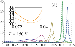
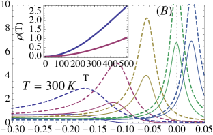
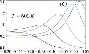
Figure 1: The density $n=.85$ and $\omega_{0}=0.25$. From left to right $\rho_{{\cal{G}}}(x)$ for energies (in units of W) $\xi=-0.3,-0.2,-0.1,0.,0.05$ for both the FL (dashed) and the ECFL(solid) theories. Inset in (A): provides an enlarged view of the $\xi=-0.1$ plots after inversion, and displays the left-skew asymmetry of the ECFL spectrum relative to the FL. Inset in (B) shows the DC resistivity $\rho(T)$ within a bubble approximation as a function of $T$ for the FL (blue) and the ECFL (red). Due to spectral redistribution, the ECFL reaches linear $T$ behaviour at a lower $T$ than the FL.

References

(1) W. Metzner and D. Vollhardt, Phys. Rev. Letts. 62, 324 (1989); A. Georges, G. Kotliar, W. Krauth and M. J. Rozenberg, Rev. Mod. Phys. 68, 13 (1996).
(2) P. W. Anderson, Science 235, 1196 (1987); Phys. Rev. B 78, 174505 (2008).
(3) B. S. Shastry, Phys. Rev. B81, 045121 (2010).
(4) J. M. Luttinger and J. C. Ward, Phys. Rev 118, 1417 (1960), J. M . Luttinger, Phys. Rev. 119, 1153 (1960);
Phys. Rev. 121, 942 (1961).
(5) A. A. Abrikosov, L. Gorkov and I. Dzyaloshinski, Methods of Quantum Field Theory in Statistical Physics , Prentice-Hall,
Englewood Cliffs, NJ (1963).
(6) This expression differs slightly from I-29 in Ref. (ECQL, ). The added terms vanish exactly due to the Pauli principle and Gutzwiller projection that eliminate states with double occupancy. They are added since they serve to usefully symmetrize
the expressions for and and thereby simplify the subsequent treatment.
(7) This choice is the essential difference from a decomposition in I Eq. (I-31). In the present case, we are able to establish adiabatic continuity with the Fermi gas as indicated in Eq. (9) below.
(8) It is important to realize that the nature of the expansion is different from that of a typical perturbative expansion, e.g. the expansion in the Hubbard model. In the present case the scales of all parameters are similar , since the large parameter of the Hubbard model has been set at at the outset. Thus should be viewed as a parameter that organizes the equations in a systematic fashion so that e.g. keeping all terms of
gives a consistent theory that is structurally analogous to the skeleton expansion at . We may then examine the nature of the solution to this order, with the expectation that the term would retain the qualitative features found at lower order. Further since couples to in Eq. (10), an expansion in should be viewed as a low density expansion.
(9) We have thus imposed the L-W theorem in Eq. (16) rather than proved it in this theory.
(10) In Eq. (14) we lump all dispersion type terms in the expression into an effective dispersion , thus writing .
(11) This functional form is based on the result for of the Hubbard model, after one sets the parameter in view of the scales of variables of the - model noted inlambda . For small energies the behaviour of the Fermi liquid noted in agd is captured in this form, and a reasonable extrapolation to large frequencies is provided.
(12) The Hilbert transform of is denoted by . Here with
and
where is the imaginary error function.
(13)In computing the various parameters self consistently, one finds that the positivity enforcing function in Eq. (26) can be dropped with very little (%) error.
(14) This gives a band width of eV that is typical of cuprates.
(15) C. M. Varma, P. B. Littlewood, S. Schmitt-Rink, E. Abrahams, and A. E. Ruckenstein
Phys. Rev. Lett. 63, 1996 (1989)
(16) This physical duality is to be understood in the sense that a highly elastic auxiliary FL over all energies, with very sharp features would lead to a small through Eq. (27), so that the ECFL spectrum would have a very large coefficient of the linear term in Eq. (26) and hence appear incoherent.