The Capra Research Program for Modelling Extreme Mass Ratio Inspirals

Abstract

Suppose a small compact object (black hole or neutron star) of mass $m$ orbits a large black hole of mass $M\gg m$. This system emits gravitational waves (GWs) that have a radiation-reaction effect on the particle’s motion. EMRIs (extreme–mass-ratio inspirals) of this type will be important GW sources for LISA. To fully analyze these GWs, and to detect weaker sources also present in the LISA data stream, will require highly accurate EMRI GW templates.

In this article I outline the “Capra” research program to try to model EMRIs and calculate their GWs ab initio, assuming only that $m\ll M$ and that the Einstein equations hold. Because $m\ll M$ the timescale for the particle’s orbit to shrink is too long for a practical direct numerical integration of the Einstein equations, and because this orbit may be deep in the large black hole’s strong-field region, a post-Newtonian approximation would be inaccurate. Instead, we treat the EMRI spacetime as a perturbation of the large black hole’s “background” (Schwarzschild or Kerr) spacetime and use the methods of black-hole perturbation theory, expanding in the small parameter $m/M$.

The particle’s motion can be described either as the result of a radiation-reaction “self-force” acting in the background spacetime or as geodesic motion in a perturbed spacetime. Several different lines of reasoning lead to the (same) basic $\mathcal{O}(m/M)$ “MiSaTaQuWa” equations of motion for the particle. In particular, the MiSaTaQuWa equations can be derived by modelling the particle as either a point particle or a small Schwarzschild black hole. The latter is conceptually elegant, but the former is technically much simpler and (surprisingly for a nonlinear field theory such as general relativity) still yields correct results.

Modelling the small body as a point particle, its own field is singular along the particle worldline, so it’s difficult to formulate a meaningful “perturbation” theory or equations of motion there. Detweiler and Whiting found an elegant decomposition of the particle’s metric perturbation into a singular part which is spherically symmetric at the particle and a regular part which is smooth (and non-symmetric) at the particle. If we assume that the singular part (being spherically symmetric at the particle) exerts no force on the particle, then the MiSaTaQuWa equations follow immediately.

The MiSaTaQuWa equations involve gradients of a (curved-spacetime) Green function, integrated over the particle’s entire past worldline. These expressions aren’t amenable to direct use in practical computations. By carefully analysing the singularity structure of each term in a spherical-harmonic expansion of the particle’s field, Barack and Ori found that the self-force can be written as an infinite sum of modes, each of which can be calculated by (numerically) solving a set of wave equations in $1{+}1$ dimensions, summing the gradients of the resulting fields at the particle position, and then subtracting certain analytically-calculable “regularization parameters”. This “mode-sum” regularization scheme has been the basis for much further research including explicit numerical calculations of the self-force in a variety of situations, initially for Schwarzschild spacetime and more recently extending to Kerr spacetime.

Recently Barack and Golbourn developed an alternative “$m$-mode” regularization scheme. This regularizes the physical metric perturbation by subtracting from it a suitable “puncture function” approximation to the Detweiler-Whiting singular field. The residual is then decomposed into a Fourier sum over azimuthal ($e^{im\varphi}$) modes, and the resulting equations solved numerically in $2{+}1$ dimensions. Vega and Detweiler have developed a related scheme that uses the same puncture-function regularization but then solves the regularized perturbation equation numerically in $3{+}1$ dimensions, avoiding a mode-sum decomposition entirely. A number of research projects are now using these puncture-function regularization schemes, particularly for calculations in Kerr spacetime.

Most Capra research to date has used 1st order perturbation theory, with the particle moving on a fixed (usually geodesic) worldline. Much current research is devoted to generalizing this to allow the particle worldline to be perturbed by the self-force, and to obtain approximation schemes which remain valid over long (EMRI-inspiral) timescales. To obtain the very high accuracies needed to fully exploit LISA’s observations of the strongest EMRIs, 2nd order perturbation theory will probably also be needed; both this and long-time approximations remain frontiers for future Capra research.

This article is dedicated to the memory of Thomas Radke, my late friend and colleague in many computational adventures.

I Introduction

An EMRI (extreme–mass-ratio inspiral) is a binary black hole (BH) system (or a binary BH/neutron-star system) with a highly asymmetric mass ratio. That is, an EMRI consists of a small compact object (a stellar-mass BH or neutron star) of mass $\mu M$ orbiting a large BH of mass $M$, with the mass ratio $\mu\ll 1$. If the small body were a test mass ($m=0$), then it would orbit on a geodesic of the large BH. However, if $m>0$, then the system emits gravitational waves (GWs), and there is a corresponding radiation-reaction influence on the small body’s motion. Calculating this motion and the emitted GWs is a long-standing research question, and is interesting both as an abstract problem in general relativity and as an essential prerequisite for the full success of LISA. LISA is expected to observe GWs from many EMRIs with $M\sim 10^{6}M_{\odot}$ and $m\sim 10M_{\odot}$ (so that $\mu\sim 10^{-5}$) Amaro-Seoan-etal-2007:LISA-IMRI-and-EMRI-review ; Gair-2009:LISA-EMRI-event-rates . To most effectively analyze this LISA data – indeed, even to detect much weaker signals that may also be present in the LISA data stream – requires accurately modelling the EMRI GWs, particularly the GW phase Porter-2009:LISA-data-analysis-overview .

The small body’s orbit may be highly relativistic, so post-Newtonian methods (see, for example, (Damour-in-Hawking-Israel-1987, , section 6.10); Blanchet-2006-living-review ; Futamase-Itoh-2007:PN-review ; Blanchet-2009:PN-review ; Schaefer-2009:PN-review and references therein) may not be accurate for this problem. Since the timescale for radiation reaction to shrink an EMRI orbit is very long (${\sim}\,\mu^{-1}M$) while the required resolution near the small body is very high (${\sim}\,\mu M$), full (nonlinear) numerical-relativity methods (see, for example, Pretorius-2007:2BH-review ; Hannam-etal-2009:Samurai-project ; Hannam-2009:2BH-review ; Hannam-Hawke-2010:2BH-in-era-of-Einstein-telescope-review ; Hinder-2010:2BH-review ; Campanelli-etal-2010:2BH-numrel-review ; Centrella-etal-2010:2BH-numrel-review and references therein) would be both prohibitively expensive and insufficiently accurate for this problem.

Instead, a variety of other approximation schemes are used to model EMRIs and their GWs. In particular, the “Capra” research program, uses the techniques of BH perturbation theory to model the EMRI spacetime ab initio as a perturbation of the massive central BH’s Schwarzschild or Kerr spacetime, making no approximations other than that the mass ratio $\mu\ll 1$. In particular, the Capra research program doesn’t make any slow-motion or weak-field approximations.

In this article I give a relatively non-technical overview of some of the highlights of the Capra research program, focusing on those aspects most relevant to explicitly calculating radiation-reaction effects in various physical systems. My goal is to give the reader some sense of the “flavor” of Capra research. The reader should have a reasonable background in general relativity and, for some parts of sections II.1, II.2, and II.4, be familiar with Green-function methods for solving linear partial differential equations (PDEs). The sections of this article are relatively independent and, with a few exceptions (which should be obvious from cross-references), can be read in any order. In sections II.2 and II.4 I have marked certain passages as somewhat more technical (analogous to the “Track 2” of Misner, Thorne, and Wheeler MTW-1973 ); this material may be skipped if the reader so desires.

This is emphatically not a comprehensive review – there are major areas of the Capra program that I only briefly mention, and others which I omit entirely. Except for some of the accuracy arguments in section IV, there’s no original research in this article. For more detailed and complete information about the Capra research program, the reader should consult any of a number of excellent review articles, notably those by Poisson Poisson-2004-living-review ; Poisson-2005-GR17-plenary ; Poisson-2009:self-force-review , Detweiler Detweiler-2005 , and Barack Barack-2009:self-force-review . The websites of recent Capra meetings Capra-2009-Bloomington-www ; Capra-2010-Waterloo-www also include archives of meeting presentations.

A key long term goal of the Capra research program is the modelling (and explicit calculation) of highly accurate orbital dynamics and GW templates for generic EMRIs. As discussed in section IV, the highest-accuracy GW templates for LISA will probably require carrying BH perturbation theory to at least 2nd order in the mass ratio $\mu$, and also using special “long-time” approximation schemes. These are ambitious goals, which are still far from being met: most Capra research to date has been devoted to the lesser – but still challenging – problem of trying to model strong-field EMRI radiation-reaction effects using 1st order perturbation theory and, to the best of my knowledge, no Capra GW templates have yet been published. I return to 2nd-order calculations in sections IV and V, but for the rest of this article I consider only 1st-order calculations.

In almost all Capra calculations to date, the small body is taken to move on a fixed geodesic worldline of the background (Schwarzschild or Kerr) spacetime, with radiation-reaction effects being manifest as an $\mathcal{O}(\mu^{2})$ “self-force” acting on the small body. Alternatively, we can view the small body as moving on a geodesic of a $\mathcal{O}(\mu)$-perturbed spacetime. These two perspectives can be shown to be fully equivalent Sago-Barack-Detweiler-2008 and are, in some ways, analogous to Eulerian versus Lagrangian approaches to fluid dynamics; we can use whichever is more convenient for any given calculation.

Another important choice in self-force analyses is whether to model the small body as a point particle or as a nonzero-sized small compact body. Modelling it as a nonzero-sized body is conceptually elegant but technically difficult. In contrast, point-particle models are technically simpler but pose difficult conceptual and foundational problems. Indeed, in a nonlinear field theory such as general relativity, the very notion of a “point particle” is difficult to formulate in a self-consistent manner Geroch-Traschen-1987 . Remarkably, it turns out that these difficulties can be overcome and, in fact, point-particle models have been used for the bulk of Capra research to date. I discuss this point further in section II.

Starting from the Einstein equations, one can derive the generic $\mathcal{O}(\mu)$ “MiSaTaQuWa” equations of motion for the small body in an arbitrary (strong-field) curved spacetime. These equations give the self-force in terms of a formal Green-function integral over the particle’s entire past motion and have now been obtained in several different ways, using both point-particle and nonzero-sized models of the small body.

It’s usually not possible to explicitly calculate the Green function appearing in the MiSaTaQuWa equations. Instead, practical computational schemes are usually based on regularizing the (singular) metric-perturbation equations for a point particle; several different ways are now known to do this. The regularized equations can then be solved (usually numerically) to actually compute the self-force for a given physical system. Because these calculations are in many cases both conceptually difficult and computationally demanding, new techniques are often first developed on simpler electromagnetic or scalar-field “model” systems. These retain many of the basic conceptual features of the gravitational case while greatly simplifying the gauge choice and the resulting computations.

We can categorize Capra self-force calculations along several dimensions of complexity:

• The background spacetime may be either Schwarzschild or Kerr.

• The field equations may be for the scalar-field, electromagnetic, or the full gravitational case.

• The small body may be stationary, in an equatorial circular orbit, in a generic (non-circular) equatorial orbit, or in a fully generic (inclined non-circular) orbit in Kerr spacetime.

The outline of the remainder of this article is as follows: In section II I discuss some of the key theoretical foundations of the Capra program including the Barack-Ori mode-sum regularization, the Detweiler-Whiting decomposition of a point particle’s metric perturbation, several different derivations of the basic 1st-order “MiSaTaQuWa” equations of motion for a small compact body moving in a curved spacetime, the Barack-Golbourn and Vega-Detweiler puncture-function regularizations and the self-force computational schemes derived from them, and the decomposition of self-force effects into conservative and dissipative parts. In section III I summarize a recent self-force calculation of Barack and Sago Barack-Sago-2010 , which provides an almost complete solution of the 1st-order self-force problem for a particle moving on a fixed geodesic orbit in Schwarzschild spacetime. In section IV I roughly estimate LISA’s accuracy requirements for GW templates, and outline some of the issues in trying to model EMRI orbital dynamics for long (orbital-decay) times to construct such templates. Finally, in section V I summarize the progress of the Capra program to date and discuss some of its likely future prospects.

Throughout this article I use $c=G=1$ units and a $(-,+,+,+)$ metric signature. I use the Penrose abstract-index notation, with $abcde$ as spacetime indices. $\delta(\cdot)$ is the Dirac $\delta$-function, $\tau$ denotes proper time along the small body’s worldline, and a subscript $p$ denotes evaluation at the small body (particle)’s current position. $\mu\ll 1$ is the EMRI system’s mass ratio and $M$ the central BH’s mass. Apart from these, the notation in this article varies somewhat from section to section; it’s always described at the start of each section.

II Theoretical Background

In this section I discuss some of the main theoretical background and formalisms which underlie the Capra research program.

A key early result of Capra research was the derivation in several different ways of the basic 1st-order equations of motion for a small compact body moving in a strong-field curved spacetime. These equations were first derived in 1997 by Mino, Sasaki, and Tanaka Mino-Sasaki-Tanaka-1997 and Quinn and Wald Quinn-Wald-1997 , and (abbreviating the authors’ names) are now known as the “MiSaTaQuWa” equations.

The MiSaTaQuWa equations involve gradients of a curved-spacetime Green function, integrated over the particle’s entire past worldline. We can rarely calculate the Green function explicitly, so the MiSaTaQuWa equations aren’t useful for practical computations. In section II.1 I discuss the “mode-sum regularization” computational scheme due originally to Barack and Ori Barack-Ori-2000 . This scheme regularizes each mode of a spherical-harmonic decomposition of the (singular) scalar-field or metric perturbation, then solves numerically for each regularized mode in $1{+}1$ dimensions. This scheme has been the basis for much further research, including many practical self-force calculations.

In 2003 Detweiler and Whiting Detweiler-Whiting-2003 found a Green-function decomposition – and a corresponding decomposition of the metric perturbation due to a small particle – into singular and radiative fields, which greatly aids understanding the self-force and related phenomena. In section II.2 I discuss this decomposition and the related Detweiler-Whiting “postulate” concerning the physical significance of the singular and radiative fields.

In section II.3 I outline how the Detweiler-Whiting postulate allows the MiSaTaQuWa equations to be derived via modelling the small body as a point particle. This derivation of the MiSaTaQuWa equations is quite simple, but it does involve the introduction of point particles and the assumption of the Detweiler-Whiting postulate.

As an alternative, in section II.4 I outline a different derivation of the MiSaTaQuWa equations, this time modelling the small body as a small nonrotating (Schwarzschild) BH. This derivation is technically more difficult than the point-particle derivation, but it avoids both the introduction of point particles and the assumption of the Detweiler-Whiting postulate.

Recently researchers have developed several new analyses of the self-force problem, leading to much more satisfactory derivations of the MiSaTaQuWa (and analogous) equations. These new analyses are fully rigorous and resolve a number of past conceptual difficulties as well as opening promising avenues for further research. I (very) briefly outline these analyses in section II.5.

Recently two groups have developed alternate “puncture-function” regularization schemes for self-force computations. Both schemes first subtract from the physical field a suitable “puncture function” approximation to the Detweiler-Whiting singular field, leaving a regular remainder field. Barack, Golbourn, and their coauthors Barack-Golbourn-2007 ; Barack-Golbourn-Sago-2007 ; Dolan-Barack-2011 developed an “$m$-mode” regularization scheme which then decomposes the perturbation equation into a Fourier sum over azimuthal ($e^{im\varphi}$) modes, and finally solves numerically for each mode in $2{+}1$ dimensions. Vega, Detweiler, and their coauthors Vega-Detweiler-2008:self-force-regularization ; Vega-etal-2009:self-force-3+1-primer have developed a different puncture-function regularization scheme that numerically solves the regularized equation directly in $3{+}1$ dimensions, avoiding a mode-sum decomposition entirely. I describe both of these schemes in section II.6.

The self force can be decomposed into conservative (time-symmetric) and dissipative (time-antisymmetric) parts. In section II.7 I discuss this decomposition and its physical significance.

II.1 The Barack-Ori Mode-Sum Regularization

The MiSaTaQuWa equations (discussed further in sections II.2–II.5) give the self-force in terms of the gradient of a curved-spacetime Green function, integrated over the entire past history of the small body. (The integral must be cut off infinitesimally before the small body’s current position.) For most physically-interesting systems we can’t explicitly calculate the Green function, so the MiSaTaQuWa equations aren’t useful for practical calculations. Instead, almost all practical self-force calculations use other regularized reformulations of the (singular) scalar-field, electromagnetic, or metric-perturbation equations.

Building on earlier suggestions of Ori Ori-1995 ; Ori-1997 , in 2000 Barack and Ori Barack-Ori-2000 proposed a practical “mode-sum” regularization of the field equations, initially for the model problem of a scalar particle moving in Schwarzschild spacetime. Barack and various coauthors Barack-2000 ; Barack-2001 ; Barack-etal-2002 ; Barack-Ori-2002 ; Barack-Lousto-2002 ; Barack-Ori-2003 soon extended this to include electromagnetic and gravitational particles in a somewhat wider class of spherically symmetric black hole spacetimes, as well as scalar-field, electromagnetic, and gravitational particles in Kerr spacetime Barack-Ori-2003:Kerr . The mode-sum regularization has been the basis for much further research including many practical self-force calculations.

To explain the mode-sum regularization, I consider the scalar-field case – this contains the essential ideas, but is technically much simpler than the full gravitational case. Thus, consider a point particle of scalar charge $q$, moving along a timelike worldline $\Gamma=\Gamma(\tau)$ in a background Schwarzschild spacetime with metric $g_{ab}$ and covariant derivative operator $\nabla_{a}$. In this section we raise and lower all indices with the background Schwarzschild metric $g_{ab}$, and we take $(t,r,\theta,\varphi)$ to be the usual Schwarzschild coordinates.

We take the scalar field $\phi$ to satisfy the usual scalar wave equation

$$\Box\phi=-4\pi q\!\int_{-\infty}^{+\infty}\!\frac{\delta^{4}\bigl{(}x^{a}-\Gamma^{a}(\tau^{\prime})\bigr{)}}{\sqrt{-g}}\,d\tau^{\prime}=:S\text{\hskip 5.0pt,}$$ (1)

where the integral extends over the entire worldline of the particle, and we define $S$ to be the source term (right hand side). We assume that if the scalar field were regular (non-singular) at the particle, it would exert a force

$$F_{a}=q\,(\nabla_{a}\phi)_{p}$$ (2)

on the particle.

The scalar wave equation (1) can be formally solved by means of a retarded Green function $\mathcal{G}(x,x^{\prime})$,

$$\phi(x)=\int_{-\infty}^{+\infty}\!\mathcal{G}\bigl{(}x,\Gamma(\tau^{\prime})\bigr{)}\,d\tau^{\prime}\text{\hskip 5.0pt,}$$ (3)

where the Green function $\mathcal{G}(x,x^{\prime})$ satisfies

$$\Box\mathcal{G}(x,x^{\prime})=-\frac{4\pi}{\sqrt{-g}}\,\delta^{4}(x^{a}-{x^{\prime}}^{a})$$ (4)

and incorporates the appropriate causality relationships.

Ignoring some terms which aren’t relevant here, the self-force on the particle at the worldline event $x=(t,r,\theta,\varphi)$ can then be shown to be given by

$$F_{a}(x)=q^{2}\!\int_{-\infty}^{x^{-}}\!\nabla_{a}\mathcal{G}\bigl{(}x;\Gamma(\tau^{\prime})\bigr{)}\,d\tau^{\prime}\text{\hskip 5.0pt,}$$ (5)

where the upper limit $x^{-}$ means that the integral extends over the entire past worldline of the particle prior to (but not including) the event $x$.

Now consider a spherical-harmonic decomposition of the scalar field $\phi$ and the self-force $F_{a}$,

$$\phi(x) = \sum_{\ell=0}^{\infty}\sum_{m=-\ell}^{+\ell}\!Y_{\ell m}(\theta,\varphi)\phi^{\ell m}(t,r)$$ (6a)

$$F_{a}(x) = \sum_{\ell=0}^{\infty}\sum_{m=-\ell}^{+\ell}\!Y_{\ell m}(\theta,\varphi)F_{a}^{\ell m}(t,r)\text{\hskip 5.0pt,}$$ (6b)

and sum over the azimuthal mode number $m$ by defining

$$F_{a}^{\ell}(t,r,\theta,\varphi)=\sum_{m=-\ell}^{+\ell}\!Y_{\ell m}(\theta,\varphi)F_{a}^{\ell m}(t,r)\text{\hskip 5.0pt,}$$ (7)

so that the self-force is given by

$$F_{a}=\sum_{\ell=0}^{\infty}F_{a}^{\ell}\text{\hskip 5.0pt.}$$ (8)

It turns out that each individual spherical-harmonic mode $F_{a}^{\ell}$ is finite, but the sum over $\ell$ of these modes in (8) diverges. However, by carefully analysing the divergence of the scalar field and its Green function near the particle, Barack and Ori showed that the related sum

$$\sum_{\ell=0}^{\infty}\left(F_{a}^{\ell}-[A_{a}L+B_{a}+C_{a}/L]\right)\text{\hskip 5.0pt,}$$ (9)

(where $L=\ell+\tfrac{1}{2}$, and where the quantities $A_{a}$, $B_{a}$, and $C_{a}$ are described below) does in fact converge and moreover, that the self-force is given by

$$F_{a}=\sum_{\ell=0}^{\infty}\left(F_{a}^{\ell}-[A_{a}L+B_{a}+C_{a}/L]\right)-Z_{a}\text{\hskip 5.0pt,}$$ (10)

where the “regularization parameters” $A_{a}$, $B_{a}$, $C_{a}$, and $Z_{a}$ are independent of $\ell$ and can be calculated semi-analytically as elliptic integrals depending on the worldline $\Gamma$ and the worldline event $x$.

[More generally, additional even-power terms $D^{(2)}_{a}\!/L^{2}$, $D^{(4)}_{a}\!/L^{4}$, $D^{(6)}_{a}\!/L^{6}$, …, can be added to the $A_{a}L+B_{a}+C_{a}/L$ inner sum in the mode-sum self-force formula (10) (with corresponding adjustments to the definition of $Z_{a}$). As discussed by Detweiler, Messaritaki, and Whiting Detweiler-Messaritaki-Whiting-2003 , if the additional regularization parameters $D^{(k)}_{a}$ can be explicitly calculated (analytically or semi-analytically), then adding these extra terms can greatly accelerate the convergence of the sum over $\ell$. I discuss the numerical treatment of this infinite sum below.]

By virtue of the spherical symmetry of the Schwarzschild background, the spherical-harmonic decomposition (6) separates the scalar wave equation (1). That is, each individual $\phi^{\ell m}(t,r)$ now satisfies a linear wave equation in $1{+}1$ dimensions on the Schwarzschild background,

$$\Box\phi^{\ell m}+V_{\ell}(r)\phi^{\ell m}=S_{\ell m}(t)\,\delta\bigl{(}r-r_{p}(t)\bigr{)}\text{\hskip 5.0pt,}$$ (11)

where the potential $V_{\ell}(r)$ and source term $S_{\ell m}(t)$ are known analytically, and where $r_{p}(t)$ is the particle’s (known) Schwarzschild radial coordinate (which is time-dependent if the worldline is anything other than a circular geodesic orbit). The wave equation (11) can then be solved numerically in the time domain to find the field $\phi^{\ell m}$.

Finally, each individual self-force mode $F_{a}^{\ell m}$ can be calculated from the $\ell m$ component of the basic force law (2),

$$F_{a}^{\ell m}=q\left(\nabla_{a}\phi^{\ell m}\right)_{p}\text{\hskip 5.0pt,}$$ (12)

and then $F_{a}^{\ell}$ can be calculated from (7).

Alternatively, we can take a frequency-domain approach, augmenting the spherical-harmonic expansions (6) with a Fourier transform in time, i.e., we can replace those expansions with

$$\phi(x) = \int\limits_{\omega}\sum_{\ell=0}^{\infty}\sum_{m=-\ell}^{+\ell}\!Y_{\ell m}(\theta,\varphi)e^{i\omega_{m}t}\phi^{\omega\ell m}(r)\,d\omega$$ (13a)

$$F_{a}(x) = \int\limits_{\omega}\sum_{\ell=0}^{\infty}\sum_{m=-\ell}^{+\ell}\!Y_{\ell m}(\theta,\varphi)e^{i\omega_{m}t}F_{a}^{\omega\ell m}(r)\,d\omega\text{\hskip 5.0pt,}$$ (13b)

and correspondingly replace the $$m$$ summation (7) with

$$F_{a}^{\ell}(t,r,\theta,\varphi)=\int\limits_{\omega}\sum_{m=-\ell}^{+\ell}\!Y_{\ell m}(\theta,\varphi)e^{i\omega_{m}t}F_{a}^{\omega\ell m}(r)\,d\omega\text{\hskip 5.0pt.}$$ (13c)

We also similarly Fourier-transform and spherical-harmonic–expand the source term (right hand side) $$S$$ in the scalar wave equation (1),

$$S(x)=\int\limits_{\omega}\sum_{\ell=0}^{\infty}\sum_{m=-\ell}^{+\ell}\!Y_{\ell m}(\theta,\varphi)e^{i\omega_{m}t}S_{\omega\ell m}(r)\,d\omega\text{\hskip 5.0pt.}$$ (13d)

The rest of the mode-sum regularization then goes through unchanged for each frequency $\omega$, and each individual scalar-field mode $\phi^{\omega\ell m}(r)$ now satisfies the ordinary differential equation

$$\frac{d^{2}\phi^{\omega\ell m}}{dr^{2}}+H(r)\frac{d\phi^{\ell m\omega}}{dr}+V_{\omega\ell}(r)\phi^{\omega\ell m}=S_{\omega\ell m}(r)\text{\hskip 5.0pt,}$$ (14)

where the coefficients $H(r)$, $V_{\omega l}(r)$, and $S_{\omega\ell m}(r)$ are again all known analytically.

The frequency-domain approach involves much simpler computations (ODEs) than the time-domain approach’s PDEs. If the particle orbit is circular, then only a single frequency is needed, and the integrals over $\omega$ are trivial. On the other hand, if the particle orbit is noncircular, many frequencies $\omega$ may be needed to adequately approximate the integrals over $\omega$.

In any case, once the individual $F^{\ell m}$ or $F^{\omega\ell m}$ are known, there remains the problem that the overall $\ell$ sum (8) is an infinite sum. For computational purposes a finite expression is needed. The solution to this lies in the known large-$\ell$ behavior Detweiler-Messaritaki-Whiting-2003 of $F_{a,\text{reg}}^{\ell}:=F_{a}^{\ell}-[A_{a}L+B_{a}+C_{a}/L]$,

$$F_{a,\text{reg}}^{\ell}=\frac{D^{(2)}_{a}}{L^{2}}+\frac{D^{(4)}_{a}}{L^{4}}+\frac{D^{(6)}_{a}}{L^{6}}+\cdots\qquad\text{for large $L$}\text{\hskip 5.0pt,}$$ (15)

where the coefficients $D^{(k)}_{a}$ are independent of $L$. [Of course, if a term $D^{(k)}_{a}\!/L^{k}$ has been added to the $A_{a}L+B_{a}+C_{a}/L$ inner sum in the mode-sum self-force formula (10), then that term is absent from the large-$L$ series (15).] We partition the overall $\ell$ sum (8) into a finite “numerical” part and an infinite “tail” part,

$$F_{a}=\sum_{\ell=0}^{\ell_{\max}}F_{a,\text{reg}}^{\ell}+\sum_{\ell=\ell_{\max}{+}1}^{\infty}F_{a,\text{reg}}^{\ell}\text{\hskip 5.0pt,}$$ (16)

where $\ell_{\max}\sim 15$–$30$ is a numerical parameter. Then, once all the $F_{a,\text{reg}}^{\ell}$ in the numerical part of the sum are known, we can fit some number (typically $2$ or $3$) of terms in the large-$\ell$ series (15) to the numerically-computed $F_{a,\text{reg}}^{\ell}$ values, and use the fitted coefficients $\{D^{(k)}_{a}\}$ to estimate the tail term.

II.2 The Detweiler-Whiting Decomposition

Suppose we model the small body as a point particle. (In this section we ignore the point-particle foundational issues mentioned in footnote 14.) Because the particle’s own field is singular along the particle worldline, it’s not obvious how to write a meaningful “perturbation” theory or formulate equations of motion there. The solution (within the framework of modelling the small body as a point particle) is to somehow regularize the field so that we have finite quantities to manipulate.

The regularization of the (retarded) field of a point-particle source near that source is a long-standing problem in mathematical physics. Dirac Dirac-1938 studied this problem for the electromagnetic field of a point charge in flat spacetime and found a decomposition of the field into a singular part which is spherically symmetric about the charge, and a “radiative” part which is regular at the charge. [We might then assume (postulate) that despite being singular, the spherically-symmetric part exerts no force on the charge. I discuss the curved-spacetime generalization of this assumption (postulate) below.] Dirac’s analysis was generalized to curved spacetime by DeWitt and Brehme DeWitt-Brehme-1960 (with a correction by Hobbs Hobbs-1968 ).

More recently, Detweiler and Whiting Detweiler-Whiting-2003 found a fully satisfactory curved-spacetime decomposition of a point particle’s field (whether scalar, electromagnetic, or gravitational) into singular and regular parts. Here I describe this decomposition for the gravitational case. Suppose we have a point mass $m$, moving (unaffected by external forces apart from self-force effects) with 4-velocity $u^{a}$ along a timelike worldline $\Gamma\,{=}\,\Gamma(\tau)$ in a “background” vacuum spacetime whose typical radius of curvature in a neighborhood of $\Gamma$ is $\mathcal{R}\gg m$. [For a LISA EMRI we might have $m\sim 10M_{\odot}$ while $\mathcal{R}\sim 10^{6}M_{\odot}$ (the massive BH’s mass).]

Suppose $\smash{{}^{(0)}\!g}_{ab}$ is the (vacuum) background metric, i.e., the spacetime metric in the absence of the particle, and $\nabla_{a}$ is the corresponding covariant derivative. Throughout this section we raise and lower indices with the background metric $\smash{{}^{(0)}\!g}_{ab}$. Let $h_{ab}$ be the metric perturbation produced by the particle, so that the physical spacetime metric is $g_{ab}=\smash{{}^{(0)}\!g}_{ab}+h_{ab}$. We introduce the standard trace-reversed metric perturbation $\bar{h}_{ab}=h_{ab}-\tfrac{1}{2}\smash{{}^{(0)}\!g}_{ab}h_{c}{}^{c}$ and impose the Lorenz gauge condition $\nabla_{a}\bar{h}^{ab}=0$ on the metric perturbation.

[The material from this point up to and including the paragraph containing equation (21) is somewhat more technical than the rest of this article and can be skipped without creating confusion.]

Up to $\mathcal{O}(m/\mathcal{R})$ accuracy, the metric perturbation satisfies the linear (wave) equation

$$\nabla^{c}\nabla_{c}\bar{h}_{ab}+2R^{c}{}_{a}{}^{d}{}_{b}\bar{h}_{cd}=T_{ab}\text{\hskip 5.0pt,}$$ (17)

where $T_{ab}$ is the particle’s ($\delta$-function) stress-energy tensor.

The (linear) perturbation equation (17) can be formally solved by introducing a suitable retarded Green function, which for events within a normal convex neighborhood of the particle (i.e., events $x^{\prime}$ which are linked to the particle event $x$ by a unique geodesic) can be written in the Hadamard form

$$\mathcal{G}^{ab}{}_{c^{\prime}d^{\prime}}(x,x^{\prime})=\mathcal{U}^{ab}{}_{c^{\prime}d^{\prime}}(x,x^{\prime})\,\delta\bigl{(}\sigma(x,x^{\prime})\bigr{)}+\mathcal{V}^{ab}{}_{c^{\prime}d^{\prime}}(x,x^{\prime})\,\theta\bigl{(}-\sigma(x,x^{\prime})\bigr{)}\text{\hskip 5.0pt,}$$ (18)

where $\theta(\cdot)$ is the Heaviside step function, Synge’s world function $\sigma(x,x^{\prime})$ is half the squared geodesic distance between the events $x$ and $x^{\prime}$, and where $\mathcal{U}^{ab}{}_{c^{\prime}d^{\prime}}(x,x^{\prime})$ and $\mathcal{V}^{ab}{}_{c^{\prime}d^{\prime}}(x,x^{\prime})$ are smooth bitensors. The first term in this decomposition is a singular “light-cone part” supported only for $\sigma=0$, i.e., only when $x^{\prime}$ lies on the past light cone of $x$. The second term is a smooth “tail part” supported only for $\sigma<0$, i.e., only when $x^{\prime}$ lies within (but not on) the past light cone of $x$. Notice that the tail part has support throughout the entire past history of the particle. Heuristically, this is because metric perturbations from any time in the particle’s past history can scatter off the background spacetime curvature and then return to the event $x$.

The resulting formal solution of the perturbation equation (17) is

$$\bar{h}^{ab}(x)=\frac{4m}{r}\,\mathcal{U}^{ab}{}_{c^{\prime}d^{\prime}}(x,x^{\prime})u^{c^{\prime}}u^{d^{\prime}}+\bar{h}_{\text{tail}}^{ab}(x)\text{\hskip 5.0pt,}$$ (19)

where $x^{\prime}$ is the intersection of $x$’s past light cone with the worldline $\Gamma$, $u^{a^{\prime}}$ is the small BH’s 4-velocity at this retarded point $x^{\prime}$, and the tail term is given explicitly by

$$\bar{h}_{\text{tail}}^{ab}(x)=4m\int_{-\infty}^{x^{\prime}}\mathcal{V}^{ab}{}_{c^{\,\hbox{\rotatebox{90.0}{\reflectbox{\small$\sim$}}}}d^{\,\hbox{\rotatebox{90.0}{\reflectbox{\small$\sim$}}}}}\bigl{(}x,\Gamma(\tau^{\,\hbox{\rotatebox{90.0}{\reflectbox{\small$\sim$}}}})\bigr{)}u^{c^{\,\hbox{\rotatebox{90.0}{\reflectbox{\small$\sim$}}}}}u^{d^{\,\hbox{\rotatebox{90.0}{\reflectbox{\small$\sim$}}}}}\,d\tau^{\,\hbox{\rotatebox{90.0}{\reflectbox{\small$\sim$}}}}$$ (20)

where the   $\sim$  accent (superscript) marks the dummy variable of integration (integrating over the worldline), and where the integral is over the particle’s entire past history prior to the retarded point $x^{\prime}$. Figure 1 illustrates the causal relationships between $\Gamma$, $x$, $x^{\prime}$, and $x^{\,\hbox{\rotatebox{90.0}{\reflectbox{\small$\sim$}}}}$. Physically, the tail term (20) models the effect of “null then scattering then null” paths from $x^{\,\hbox{\rotatebox{90.0}{\reflectbox{\small$\sim$}}}}$ to $x$ (shown in blue in figure 1, where metric perturbations from the event $x^{\,\hbox{\rotatebox{90.0}{\reflectbox{\small$\sim$}}}}$ scatter off the background spacetime curvature and then return to the event $x$.

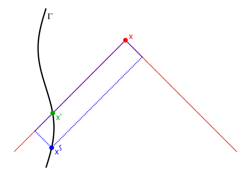
Figure 1: This figure shows (in black) the particle’s timelike geodesic worldline $\Gamma$, (in red) a nearby “field” event $x$ and its past lightcone, (in green) the event $x^{\prime}$ where this lightcone intersects the worldline $\Gamma$, (in blue) an event $x^{\,\hbox{\rotatebox{90.0}{\reflectbox{\small$\sim$}}}}$ on $\Gamma$ in the past of $x^{\prime}$, and (with blue dashed lines) two possible “null then scattering then null” paths from $x^{\,\hbox{\rotatebox{90.0}{\reflectbox{\small$\sim$}}}}$ to $x$ (these are modelled by the tail term (20)), where (heuristically) metric perturbations from the event $x^{\,\hbox{\rotatebox{90.0}{\reflectbox{\small$\sim$}}}}$ scatter off the background curvature before returning to event $x$.

The Detweiler-Whiting “singular” part of the metric perturbation is then (defined to be)

$$\bar{h}_{S}^{ab}(x)=\frac{2m}{r}\,\mathcal{U}^{ab}{}_{c^{\prime}d^{\prime}}(x,x^{\prime})u^{c^{\prime}}u^{d^{\prime}}+\frac{2m}{r}\,\mathcal{U}^{ab}{}_{c^{\prime\prime}d^{\prime\prime}}(x,x^{\prime\prime})u^{c^{\prime\prime}}u^{d^{\prime\prime}}-2m\!\int_{x^{\prime}}^{x^{\prime\prime}}\!\mathcal{V}^{ab}{}_{c^{\,\hbox{\rotatebox{90.0}{\reflectbox{\small$\sim$}}}}d^{\,\hbox{\rotatebox{90.0}{\reflectbox{\small$\sim$}}}}}\bigl{(}x,\Gamma(\tau^{\,\hbox{\rotatebox{90.0}{\reflectbox{\small$\sim$}}}})\bigr{)}u^{c^{\,\hbox{\rotatebox{90.0}{\reflectbox{\small$\sim$}}}}}u^{d^{\,\hbox{\rotatebox{90.0}{\reflectbox{\small$\sim$}}}}}\,d\tau^{\,\hbox{\rotatebox{90.0}{\reflectbox{\small$\sim$}}}}\text{\hskip 5.0pt,}$$ (21)

where (as shown in figure 2) the events $x^{\prime}$ and $x^{\prime\prime}$ are respectively the intersections of the past and future light cones of the event $x$ with the particle worldline $\Gamma$.

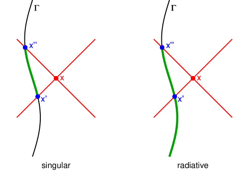
Figure 2: This figure shows the causal properties of the Detweiler-Whiting singular and radiative fields. Each subfigure shows (in black) the particle’s timelike geodesic worldline $\Gamma$, (in red) a nearby “field” event $x$ and its past and future lightcones, (in blue) the events $x^{\prime}$ (past) and $x^{\prime\prime}$ (future) where this lightcone intersects the worldline $\Gamma$, and (in green) the region of the worldline which affects the Detweiler-Whiting singular or radiative fields.

Detweiler and Whiting showed that the (singular) field $\bar{h}_{S}^{ab}$ defined in this manner satisfies the same metric-perturbation equation (17) as the physical (retarded) perturbation $\bar{h}^{ab}$, and furthermore that $\bar{h}_{S}^{ab}$ is “just as singular” as $\bar{h}^{ab}$ on the worldline $\Gamma$. That is, they showed that the “radiative” field

$$\bar{h}_{R}^{ab}(x)=\bar{h}^{ab}(x)-\bar{h}_{S}^{ab}(x)$$ (22)

is in fact smooth on the worldline $\Gamma$ (as well as everywhere else). Notice also that the radiative field satisfies the homogeneous form of the metric-perturbation equation (17).

The Detweiler-Whiting singular and radiative fields have unusual causal properties, illustrated in figure 2: the singular field depends on the particle’s history only between the events $x^{\prime}$ and $x^{\prime\prime}$, while the radiative field depends on the particle’s entire past history up to the advanced event $x^{\prime\prime}$. However, in the limit that the event $x$ approaches the worldline $\Gamma$, the radiative field then depends only on the particle’s past history.

The Detweiler-Whiting singular field $\bar{h}_{S}^{ab}(x)$ is spherically symmetric at the particle. That is, it can be shown that if we average the gradient of this field over a 2-sphere of radius $\epsilon$ centered on the particle (as seen in the particle’s instantaneous rest frame), then take the limit $\epsilon\to 0$, this average vanishes. This motivates the Detweiler-Whiting postulate: the singular field exerts no force on the particle; the self-force arises entirely from the action of the (regular) radiative field. This postulate gives valuable conceptual insight into how the self force “works”. This postulate is also closely linked to the MiSaTaQuWa equations (I discuss this in the next paragraph and in section II.3) and to puncture-function regularizations and computational schemes for the self force (I discuss these in section II.6).

Unfortunately, because the field is singular at the particle, the simple averaging argument described in the previous paragraph doesn’t constitute a rigorous proof of the Detweiler-Whiting postulate. However, the Detweiler-Whiting postulate is closely linked to the MiSaTaQuWa equations: if we assume the Detweiler-Whiting postulate, then the MiSaTaQuWa equations follow almost immediately via the argument outlined in section II.3. Because of this close linkage, we can reverse the direction of logical implication and argue that the validity of the MiSaTaQuWa equations (which are now well-established via the rigorous derivations discussed in sections II.4 and II.5) supports the correctness of the Detweiler-Whiting postulate. That is, we can argue that the Detweiler-Whiting postulate must be valid, since it is central to a derivation (the one outlined in section II.3) which leads to a correct result (the MiSaTaQuWa equations). While not a completely rigorous proof, this argument strongly supports the validity of the Detweiler-Whiting postulate.

Harte Harte-2006:EM-self-force ; Harte-2008 ; Harte-2009 ; Harte-2010 and Pound Pound-PhD ; Pound-2010a ; Pound-2010b have recently given rigorous proofs of the Detweiler-Whiting postulate (somewhat generalized in some cases).

II.3 Deriving the MiSaTaQuWa Equations via Modelling the Small Body as a Point Particle

If we ignore the foundational issues of point particles, then the Detweiler-Whiting postulate provides a relatively easy route to the MiSaTaQuWa equations: the (Detweiler-Whiting) statement that the self-force arises solely from the action of the (regular) radiative field is equivalent to the statement that the particle moves on a geodesic of the background metric perturbed by this radiative field, i.e., $\smash{{}^{(0)}\!g}_{ab}+h^{R}_{ab}$. The particle’s 4-acceleration is thus given by

$$a^{a}=\bigl{(}\smash{{}^{(0)}\!g}^{ab}+u^{a}u^{b}\bigr{)}\bigl{(}\tfrac{1}{2}\nabla_{b}h^{R}_{cd}-\nabla_{d}h^{R}_{bc}\bigr{)}u^{c}u^{d}\text{\hskip 5.0pt.}$$ (23)

It’s now easy to show that on the particle’s worldline $\Gamma$,

$$\nabla_{c}h^{R}_{ab}=-4m\bigl{(}u_{(a}R_{b)dce}+R_{adbe}u_{c}\bigr{)}u^{d}u^{e}+\nabla_{c}h^{\text{tail}}_{ab}\text{\hskip 5.0pt.}$$ (24)

Substituting (24) into (23) then gives the MiSaTaQuWa equations

$$a^{a}=\bigl{(}\smash{{}^{(0)}\!g}^{ab}+u^{a}u^{b}\bigr{)}\bigl{(}\tfrac{1}{2}h^{\text{tail}}_{cdb}-h^{\text{tail}}_{bcd}\bigr{)}u^{c}u^{d}\text{\hskip 5.0pt.}$$ (25)

where we define $h^{\text{tail}}_{abc}=\nabla_{c}h^{\text{tail}}_{ab}$. The corresponding dynamical equations of motion for the particle are

$$u^{b}\nabla_{b}u^{a}=a^{a}\text{\hskip 5.0pt.}$$ (26)

Notice that the metric $\smash{{}^{(0)}\!g}_{ab}+h^{R}_{ab}$ is smooth on the particle worldline $\Gamma$. Moreover, because $\smash{{}^{(0)}\!g}_{ab}$ is a vacuum solution of the Einstein equations everywhere and $h^{R}_{ab}$ satisfies the homogeneous form of the perturbation equation (17), the metric $\smash{{}^{(0)}\!g}_{ab}+h^{R}_{ab}$ is also a vacuum solution of the Einstein equations everywhere. This gives what Poisson Poisson-2005-GR17-plenary describes as “a compelling interpretation” to the condition (23): the particle moves on a geodesic of the vacuum spacetime with metric $\smash{{}^{(0)}\!g}_{ab}+h^{R}_{ab}$. Unfortunately, this metric doesn’t coincide with the actual physical spacetime metric $\smash{{}^{(0)}\!g}_{ab}+h_{ab}$.

II.4 Deriving the MiSaTaQuWa Equations via Modelling the Small Body as a Black Hole

This point-particle derivation of the MiSaTaQuWa equations is concise, but depends crucially on the Detweiler-Whiting postulate. In this section I outline a different derivation, based on modelling the small body as a BH. This derivation doesn’t require the assumption of the Detweiler-Whiting postulate but it (this derivation) is technically much more involved than the point-particle derivation. This derivation is originally due to Mino, Sasaki, and Tanaka Mino-Sasaki-Tanaka-1997 ; my presentation here is based on that of Poisson’s GR17 plenary lecture Poisson-2005-GR17-plenary .

In this section I adopt the same notation as in the point-particle derivation (section II.3) except that the small body is no longer modelled as a point particle. Because the small body is (locally) free-falling, its motion is actually independent of its internal structure (ignoring spin and tidal effects). This “effacement of internal structure” is a fundamental property of general relativity (not shared by most other relativistic gravity theories) and is discussed in detail in Damour’s fascinating review article in the Three Hundred Years of Gravitation volume Damour-in-Hawking-Israel-1987 . In view of this property, we are free to choose the small body’s internal structure for maximum convenience in our analysis; here we choose it to be a nonrotating (Schwarzschild) BH.

Our analysis will be based on matched asymptotic expansions of the spacetime metric: Sufficiently far from the small BH (the “far zone”), the metric is that of the background spacetime, perturbed by the presence of the small BH,

$$g_{ab}=g^{\text{background}}_{ab}+\mathcal{O}\bigl{(}m/r\bigr{)}\text{\hskip 5.0pt.}$$ (27)

Sufficiently near to the small BH (the “near zone”), the metric is that of the small (Schwarzschild) BH perturbed by the tidal field of the background spacetime,

$$g_{ab}=g^{\text{Schwarzschild}}_{ab}+\mathcal{O}\bigl{(}(r/\mathcal{R})^{2}\bigr{)}\text{\hskip 5.0pt.}$$ (28)

Since $m\ll\mathcal{R}$, there exists an intermediate “matching zone” where $m/r\ll 1$ and $r/\mathcal{R}\ll 1$, and hence both the expansions (27) and (28) are simultaneously valid. In that region these expansions must represent the same vacuum solution of the Einstein equations (modulo gauge choice). The small BH’s motion is then determined by the matching conditions.

[The material from this point up to the start of section II.4.3 is somewhat more technical than the rest of this article and can be skipped without creating confusion.]

We begin by introducing suitable retarded coordinates centered on the worldline $\Gamma$: $v$ is a backwards null coordinate constant on each ingoing null cone centered on $\Gamma$ (and is equal to proper time on $\Gamma$), and $r$ is an affine parameter on the cone’s null generators. In this section I use $ijk$ as Penrose abstract indices ranging over the spatial (non-$v$) coordinates only. The angular coordinates $\Omega^{i}=x^{i}/r$ are constant on each generator (one can think of $\Omega^{i}$ as spatial coordinates on a 2-sphere centered on the small BH).

II.4.1 The Near-Zone Metric

For present purposes it suffices to approximate the spacetime metric sufficiently near the small BH (the “near zone”) by that of a Schwarzschild BH subject to a quadrupole perturbation. In a suitable perturbation $(\tilde{v},\tilde{x}{=}\tilde{r}\tilde{\Omega}^{i})$ of the coordinates $(v,x^{i}{=}r\Omega^{i})$, the null-null component of the near-zone perturbed spacetime metric is

$$g^{\text{near}}_{\tilde{v}\tilde{v}} = -\left(1-\frac{2m}{\tilde{r}}\right)$$ (29)

$$-\,\tilde{r}^{2}\!\left(1-\frac{2m}{\tilde{r}}\right)^{\!\!2}\mathcal{E}_{ij}\tilde{\Omega}^{i}\tilde{\Omega}^{j}+\mathcal{O}\bigl{(}(\tilde{r}/\mathcal{R})^{3}\bigr{)}\text{\hskip 5.0pt,}$$

where $\mathcal{E}_{ij}=C_{vivj}=\mathcal{O}(1/\mathcal{R}^{2})$ are the electric components of the Weyl tensor $C_{abcd}$; these components measure the tidal distortion induced by the background spacetime.

II.4.2 The Far-Zone Metric

Sufficiently far from the small BH (i.e., in the “far zone”), the null-null component of the background metric is

$$\smash{{}^{(0)}\!g}_{vv}=-\bigl{(}1+2ra_{i}\Omega^{i}+r^{2}\mathcal{E}_{ij}\Omega^{i}\Omega^{j}\bigr{)}+\mathcal{O}\bigl{(}(r/\mathcal{R})^{3}\bigr{)}\text{\hskip 5.0pt,}$$ (30)

where $\mathcal{E}_{ij}$ are once again the electric components of the Weyl tensor, evaluated on $\Gamma$.

The metric perturbation $\bar{h}_{ab}$ produced by the small BH satisfies the linear perturbation equation (17), with $T_{ab}=0$ in the far zone. Assuming that the far zone lies within a normal convex neighborhood of the small BH, it can be shown that the null-null component of the far-zone perturbed spacetime metric is

$$g^{\text{far}}_{vv} = -\left(1-\frac{2m}{r}\right)$$ (31)

$$+h^{\text{tail}}_{uu}$$

$$+r\bigl{(}2m\mathcal{E}_{ij}\Omega^{i}\Omega^{j}-2a_{i}\Omega^{i}+h^{\text{tail}}_{uuu}+h^{\text{tail}}_{uui}\Omega^{i}\bigr{)}$$

$$-r^{2}\mathcal{E}_{ij}\Omega^{i}\Omega^{j}$$

$$+\mathcal{O}\bigl{(}(m/\mathcal{R})(r/\mathcal{R})^{2}\bigr{)}+\mathcal{O}\bigl{(}(r/\mathcal{R})^{3}\bigr{)}\text{\hskip 5.0pt.}$$

Differentiating the tail term (20), we find that in terms of the original (physical) retarded Green function $\mathcal{G}^{ab}{}_{c^{\prime}d^{\prime}}(x,x^{\prime\prime})$, $h^{\text{tail}}_{abc}$ is given by

$$h^{\text{tail}}_{abc}=4m\int_{-\infty}^{{x^{\prime}}^{-}}\nabla_{c}\left(\mathcal{G}_{aba^{\,\hbox{\rotatebox{90.0}{\reflectbox{\small$\sim$}}}}b^{\,\hbox{\rotatebox{90.0}{\reflectbox{\small$\sim$}}}}}-\tfrac{1}{2}\smash{{}^{(0)}\!g}_{ab}\mathcal{G}^{d}{}_{da^{\,\hbox{\rotatebox{90.0}{\reflectbox{\small$\sim$}}}}b^{\,\hbox{\rotatebox{90.0}{\reflectbox{\small$\sim$}}}}}\right)(x,x^{\,\hbox{\rotatebox{90.0}{\reflectbox{\small$\sim$}}}})u^{a^{\,\hbox{\rotatebox{90.0}{\reflectbox{\small$\sim$}}}}}u^{b^{\,\hbox{\rotatebox{90.0}{\reflectbox{\small$\sim$}}}}}\,d\tau^{\,\hbox{\rotatebox{90.0}{\reflectbox{\small$\sim$}}}}\text{\hskip 5.0pt,}$$ (32)

where the upper integration limit ${x^{\prime}}^{-}$ means that the integral extends over the entire past worldline of the small BH prior to (but not including) the event $x^{\prime}$. By cutting off the integration infinitesimally before $x^{\prime}$ we include the (regular) tail part of the Green function and exclude the (singular) light-cone part. As a result, $h^{\text{tail}}_{abc}$ is finite (although generally only $C^{0}$, i.e., continuous but not differentiable) on the worldline.

II.4.3 Matching

The coordinate transformation between the near-zone coordinates $(\tilde{v},\tilde{x}^{i}{=}\tilde{r}\tilde{\Omega}^{i})$ and the far-zone coordinates $(v,x^{i}{=}r\Omega^{i})$ can be computed explicitly (up to sufficient orders in the small-in-the-matching-zone quantities $m/\mathcal{R}$ and $r/\mathcal{R}$) in terms of $h^{\text{tail}}_{ab}$, its integrals and gradients, and $\mathcal{E}_{ij}$. Using this to transform the far-zone metric into the near-zone coordinates gives the null-null metric component

$$g^{\text{far}}_{\tilde{v}\tilde{v}} = -\left(1-\frac{2m}{\tilde{r}}\right)$$ (33)

$$-2\tilde{r}\left(a_{i}-\tfrac{1}{2}h^{\text{tail}}_{uui}+h^{\text{tail}}_{uiu}\right)\tilde{\Omega}^{i}$$

$$+(4m\tilde{r}-\tilde{r}^{2})\mathcal{E}_{ij}\tilde{\Omega}^{i}\tilde{\Omega}^{j}$$

$$+\mathcal{O}\bigl{(}(m/\mathcal{R})(\tilde{r}/\mathcal{R})^{2}\bigr{)}+\mathcal{O}\bigl{(}(\tilde{r}/\mathcal{R})^{3}\bigr{)}\text{\hskip 5.0pt.}$$

Requiring that this match the same near-zone metric component (29) up to $\mathcal{O}(m/\mathcal{R})$ now gives the 3-acceleration of the small BH’s worldline as

$$a_{i}=\tfrac{1}{2}h^{\text{tail}}_{uui}-h^{\text{tail}}_{uiu}\text{\hskip 5.0pt,}$$ (34)

from which the MiSaTaQuWa equations (25) follow directly.

Although the full derivation (including all the steps I’ve omitted in this brief synopsis) is somewhat lengthy, it can be made quite rigorous, requiring no unproven assumptions about the physical system.

II.5 Other Derivations of the MiSaTaQuWa Equations

In this section I briefly mention a number of other derivations of the MiSaTaQuWa equations. In the interests of keeping this review both short and broadly accessible, I won’t describe any of these derivations in detail.

As well as the matched-asymptotic-expansions derivation outlined in section II.4, Mino, Sasaki, and Tanaka Mino-Sasaki-Tanaka-1997 also gave another derivation based on an extension of the electromagnetic radiation-reaction analysis of DeWitt and Brehme DeWitt-Brehme-1960 .

Quinn and Wald Quinn-Wald-1997 took an axiomatic approach, showing that the electromagnetic self force can be derived by (i) using a “comparison axiom” which relates the electromagnetic force acting on charged particles with the same charge and 4-acceleration in two possibly-different spacetimes, and in addition (ii) assuming that in Minkowski spacetime the half-advanced, half-retarded electromagnetic field exerts no force on a uniformly accelerating charged particle. Quinn and Wald also derived the gravitational self force (the MiSaTaQuWa equations) using a similar set of axioms.

Building on earlier work by Harte Harte-2006:EM-self-force ; Harte-2008 ; Harte-2009 ; Harte-2010 , Gralla, Harte, and Wald Gralla-Harte-Wald-2009 have recently provided a rigorous rederivation of the classical (DeWitt-Brehme) electromagnetic self-force based on taking the limit of a 1-parameter family of spacetimes corresponding to the small body being “scaled down” in charge and mass simultaneously. (Harte’s analysis also includes a rigorous proof of a generalized form of the Detweiler-Whiting postulate for the scalar-field and electromagnetic cases, and for the linearized Einstein equations.) Gralla and Wald Gralla-Wald-2008 have rederived the gravitational self-force (the MiSaTaQuWa equations) based on a similar technique; here the small body is “scaled down” in size and mass simultaneously. Both of these derivations are mathematically rigorous and make no assumptions beyond the existence and appropriate smoothness and limit properties of the 1-parameter families of spacetimes.

Pound Pound-PhD ; Pound-2010a ; Pound-2010b has reviewed various derivations of the MiSaTaQuWa equations (including both the ones I’ve outlined here, and others) and developed several new mathematical techniques for analyzing the self-force problem. Using these, he has rederived the MiSaTaQuWa equation in a highly rigorous manner. His analysis includes a rigorous proof of the (gravitational) Detweiler-Whiting postulate and also provides many valuable insights into future directions for the Capra research program; I outline some of these “future directions” in section V.2.

II.6 Puncture-Function Regularizations

In this section I describe two recently-developed alternate regularization schemes for self-force computations. Both schemes begin by considering a “residual field”, defined as the difference between the particle’s physical field and a suitably chosen “puncture function” which approximates the particle’s Detweiler-Whiting singular field near the particle. By construction, the residual field is finite (although of limited differentiability) at the particle position, and it yields the correct self-force in the force law (2). The residual field satisfies a scalar wave equation similar to the usual one (1), except that by construction the right hand side is now a nonsingular “effective source” that can be calculated analytically. I describe the puncture function, the effective source, and the basic outline of how they can be used to regularize the (singular) field equation in section II.6.1.

The puncture function and effective source are constructed to have certain specified properties near to the particle. Their behavior far from the particle can equivalently be described as either (i) they are undefined far from the particle but the computational scheme is formulated so as not to make use of them there, or (ii) they are defined everywhere but vanish (or are negligibly small) far from the particle. Following Wardell and his colleagues Wardell-PhD ; Ottewill-Wardell-2008 ; Ottewill-Wardell-2009 ; Ottewill-Wardell-2010 ; Wardell-Vega-2011:generic-effective-source ; Vega-Wardell-Diener-2011:effective-source-for-self-force , I use the terminology (i); note that some other authors use the terminology (ii).

Given the puncture function and effective source, Barack and Golbourn’s “$m$-mode” scheme Barack-Golbourn-2007 ; Barack-Golbourn-Sago-2007 ; Dolan-Barack-2011 does a Fourier decomposition of the resulting equation into azimuthal ($e^{im\varphi}$) modes, and uses a “world tube” technique to remove any dependence on the puncture function or effective source far from the particle. The authors then solve numerically for each $m$-mode of the residual field (using a time-domain numerical evolution in $2{+}1$ dimensions for each mode), and compute the final self-force by summing over all the modes’ contributions. I discuss the Barack-Golbourn $m$-mode scheme further in section II.6.2.

Vega and Detweiler Vega-Detweiler-2008:self-force-regularization ; Vega-etal-2009:self-force-3+1-primer take a different approach: Given the puncture function and effective source, they introduce a smooth “window function” to remove any dependence on the puncture function or effective source far from the particle, then numerically solve the resulting equation directly in $3{+}1$ dimensions. I discuss the Vega-Detweiler scheme further in section II.6.3.

For either scheme, there are actually many possible choices for the puncture function and effective source. These differ in their tradeoffs between the difficulty of analytically calculating the puncture function and effective source, and how accurately the puncture function approximates the particle’s Detweiler-Whiting singular field (and correspondingly, how small the effective source is and how smooth the puncture function and effective source are at the particle). I discuss this further in section II.6.4.

Throughout this section we consider a point particle of scalar charge $q$, moving along a timelike worldline $\Gamma$ in (say) Kerr spacetime, whose typical radius of curvature in a neighborhood of $\Gamma$ is $\mathcal{R}$.

II.6.1 The Basic Puncture-Function Scheme

In this section I describe the basic puncture-function regularization in its simplest form. This is directly applicable to the Barack-Golbourn $m$-mode scheme discussed in section II.6.2 but is slightly modified for the Vega-Detweiler scheme discussed in section II.6.3.

We take the scalar field $\phi$ to satisfy the usual scalar wave equation (1). In general the Detweiler-Whiting singular field $\phi^{S}$ isn’t known analytically but, by careful analysis of the scalar field’s singularity structure near the particle, we can construct approximations to the singular field. Thus, we define an “$n$th order puncture function” $\phi^{S(n)}$ as a specific approximation – one that is known analytically – to the Detweiler-Whiting singular field $\phi^{S}$ near the particle, which satisfies

$$\phi^{S(n)}-\phi^{S}=\mathcal{O}\bigl{(}|\lambda|^{n-1}\bigr{)}$$ (35)

near the particle, where $\lambda$ is (roughly) the geodesic distance from the particle (see Dolan-Barack-2011 for a precise definition). Notice that at this point, the puncture function need only be defined near the particle; in practice, it’s usually only defined within at most a normal convex neighborhood of the particle worldline. I discuss the construction of the puncture function further in section II.6.4.

We define the “residual” field

$$\phi^{R(n)}=\phi-\phi^{S(n)}$$ (36)

near the particle. The residual field is $C^{n-2}$ at the particle (and $C^{\infty}$ elsewhere near the particle) and satisfies the wave equation

$$\Box\phi^{R(n)}=S^{\text{eff}(n)}\text{\hskip 5.0pt,}$$ (37)

with the “effective source” $S^{\text{eff}(n)}$ given by

$$S^{\text{eff}(n)}=-\Box\phi^{S(n)}-4\pi q\!\int_{-\infty}^{+\infty}\!\frac{\delta^{4}\bigl{(}x^{a}-\Gamma^{a}(\tau^{\prime})\bigr{)}}{\sqrt{-g}}\,d\tau^{\prime}\text{\hskip 5.0pt,}$$ (38)

where as in section II.1, the integral extends over the entire worldline of the particle. In general the effective source is $\mathcal{O}\bigl{(}\lambda^{n-3}\bigr{)}$ at the particle (and $C^{\infty}$ elsewhere near the particle).

The subtraction in the effective-source definition (38) can’t be evaluated numerically (both terms are singular at the particle), but it can be evaluated analytically using a (lengthy) series-expansion analysis of the field’s singularity structure. I discuss this further in section II.6.4.

If $\phi^{S(n)}$ is a sufficiently good approximation to the true Detweiler-Whiting singular field $\phi^{S}$ near the particle (i.e., if the order $n$ is large enough), and the Detweiler-Whiting postulate holds (i.e., the singular field exerts no force on the particle), then it’s easy to see that $q\nabla\phi^{R(n)}$ at the particle position gives precisely the desired self-force acting on the particle. Thus (apart from the difficulties outlined in the next two paragraphs) the self-force can be calculated by analytically calculating the effective source, then numerically solving the wave equations (37), and then finally taking the gradient of $\phi^{R(n)}$ at the particle position.

Accurately solving the wave equation (37) is made more difficult by the limited differentiability of the effective source and residual field at the particle. With standard finite differencing methods, this limited differentiability limits the order of finite-differencing convergence attainable very near the particle. Current research is exploring a variety of techniques to alleviate this problem including ignoring it (i.e., simply accepting the lower order of convergence), modifying the finite differencing scheme near the particle, and using finite-element or domain-decomposition pseudospectral methods that naturally accommodate well-localized non-differentiability in the fields Sopuerta-etal-2006 ; Sopuerta-Laguna-2006 ; Canizares-Sopuerta-2009a ; Canizares-Sopuerta-2009b ; Vega-etal-2009:self-force-3+1-primer .

Another difficulty with puncture-function regularization schemes is that in general the puncture function and effective source are only defined within at most a normal convex neighborhood of the particle whereas the physically appropriate boundary conditions for the wave equation (37) are applied (to the physical field $\phi$) at infinity. The Barack-Golbourn $m$-mode scheme and the Vega-Detweiler scheme take very different approaches to resolving this difficulty; I discuss these in (respectively) sections II.6.2 and II.6.3 below.

II.6.2 The Barack-Golbourn $m$-mode Scheme

The Barack-Golbourn $m$-mode scheme for self-force computation Barack-Golbourn-2007 ; Barack-Golbourn-Sago-2007 ; Dolan-Barack-2011 begins by defining the puncture function $\phi^{S(n)}$ and effective source $S^{\text{eff}(n)}$ exactly as just described (section II.6.1). The authors then decompose the residual field $\phi^{R(n)}$ and effective source $S^{\text{eff}(n)}$ into Fourier series in the azimuthal ($\varphi$) direction,

$$\phi^{R(n)}(x) = \sum_{m=-\infty}^{\infty}\!\phi^{R(n)}_{m}(t,r,\theta)e^{im\varphi}$$ (39a)

$$S^{\text{eff}(n)}(x) = \sum_{m=-\infty}^{\infty}\!S^{\text{eff}(n)}_{m}(t,r,\theta)e^{im\varphi}$$ (39b)

$$\phi(x) = \sum_{m=-\infty}^{\infty}\!\phi_{m}(t,r,\theta)e^{im\varphi}\text{\hskip 5.0pt.}$$ (39c)

Since we’re working on a Kerr background, the wave equation (37) now separates, so that each (complex) residual-field $m$-mode $\phi^{R(n)}_{m}(t,r,\theta)$ satisfies a modified wave equation

$$\Box_{m}\phi^{R(n)}_{m}=S^{\text{eff}(n)}_{m}$$ (40)

in $2{+}1$ dimensions, where the operator $\Box_{m}$ is easily derived analytically and where the effective-source $m$ modes are given explicitly by

$$S^{\text{eff}(n)}_{m}(t,r,\theta)=\frac{1}{2\pi}\int_{-\pi}^{\pi}S^{\text{eff}(n)}(t,r,\theta,\varphi^{\prime})e^{-im\varphi^{\prime}}\,d\varphi^{\prime}\text{\hskip 5.0pt.}$$ (41)

This integral can be done analytically in some cases, but otherwise must be done numerically.

There still remains the difficulty that the puncture function and effective source are only defined near the particle, while the physical field $\phi$ has has outgoing-wave boundary conditions at infinity. To resolve this problem, the authors introduce a worldtube (whose size is a numerical parameter, and shouldn’t be “too large” in a sense described below) whose interior contains the particle worldline $\Gamma$. The authors then define a new “numerical” field

$$\phi^{N(n)}_{m}=\left\{\begin{array}[]{ll}\phi^{R(n)}_{m}&\text{inside the worldtube}\\ \phi_{m}&\text{outside the worldtube}\text{\hskip 5.0pt,}\end{array}\right.$$ (42)

and solve numerically for this. The numerical field evidently satisfies the equations

$$\Box_{m}\phi^{N(n)}_{m}=\left\{\begin{array}[]{ll}S^{\text{eff}(n)}_{m}&\text{inside the worldtube}\\ 0&\text{outside the worldtube}\text{\hskip 5.0pt.}\end{array}\right.$$ (43)

Equivalently, one could say that the authors numerically solve the equations

$$\Box_{m}\phi^{R(n)}_{m} =S^{\text{eff}(n)}_{m}$$ inside the worldtube (44a)

$$\Box_{m}\phi_{m} =0$$ outside the worldtube (44b)

$$\phi^{R(n)}_{m} =\phi_{m}-\phi^{S(n)}_{m}$$ on the worldtube boundary  . (44c)

The authors solve the piecewise modified wave equation (40) numerically for each $m$ using a standard time-domain finite-difference numerical evolution code in $2{+}1$ dimensions. The authors use arbitrary initial data on a large domain, in the same manner discussed in section III.4 below.

[In a finite-difference numerical code, the piecewise aspect of the equations (44) is trivial to implement Barack-Golbourn-2007 ; Dolan-Barack-2011 : the code stores the grid function $\phi^{N(n)}_{m}$, and for each finite differencing operation, checks if the finite difference molecule crosses the worldtube boundary. If so, then the code “adjusts” the grid function values being finite differenced (which in this case might well be a temporary copy of a molecule-sized region of the actual grid function $\phi^{N(n)}_{m}$) as appropriate using (44c).]

With this scheme neither the puncture function nor the effective source are ever needed more than a short distance (the maximum finite-difference molecule size) outside the worldtube. Hence, so long as the worldtube isn’t too large, it’s not a problem that the puncture function and effective source aren’t defined far from the particle. Outside the worldtube, the piecewise equations (44) reduce to $\Box_{m}\phi_{m}=0$, so it’s easy to impose the appropriate outgoing-radiation outer boundary conditions.

Finally, the authors show that the self-force $F_{\text{self}}^{a}$ is given by

$$F_{\text{self}}^{a}(\tau)=q\sum_{m=0}^{\infty}\!\Biggl{.}\left(\nabla^{a}\tilde{\phi}^{R(n)}_{m}\right)\Biggr{|}_{\Gamma(\tau)}\text{\hskip 5.0pt,}$$ (45)

where the gradient is evaluated at the particle, and where the real fields $\tilde{\phi}^{R(n)}_{m}$ are defined by

$$\tilde{\phi}^{R(n)}_{m}=\left\{\begin{array}[]{ll}\phi^{R(n)}_{m}&\text{if $m=0$}\\ 2\text{Re}\left(\phi^{R(n)}_{m}e^{im\varphi}\right)&\text{if $m>0$}\text{\hskip 5.0pt.}\end{array}\right.$$ (46)

The infinite sum over $m$ in the self-force law (45) can be approximated with a finite computation using a tail-fitting procedure analogous to that described in section II.1.

The Barack-Golbourn $m$-mode scheme provides a practical and efficient route to self-force computations for a variety of physical systems. It is currently the basis for a number of such calculations. Where the original mode-sum scheme described in section II.1 reduced the self-force problem to the numerical solution of a 2-dimensional set of PDEs in $1{+}1$ dimensions, the $m$-mode scheme reduces the self-force problem to the solution of a 1-dimensional set of PDEs in $2{+}1$ dimensions. Both schemes have the major advantage that the problem-domain size, grid resolution, and/or other numerical parameters can be varied from one PDE to another. This greatly increases the efficiency of the numerical solutions.

II.6.3 The Vega-Detweiler Scheme

The Vega-Detweiler scheme for self-force computation Vega-Detweiler-2008:self-force-regularization ; Vega-etal-2009:self-force-3+1-primer takes a somewhat different approach: it begins by defining the puncture function $\phi^{S(n)}$ and effective source $S^{\text{eff}(n)}$ exactly as described in section II.6.1. The authors then introduce a real $C^{\infty}$ “window function” $W$ chosen (in a manner described further below) such that

$$W=1+\mathcal{O}\bigl{(}(\lambda/\mathcal{R})^{4}\bigr{)}$$ (47)

near the particle, and $W\to 0$ “sufficiently fast” (i.e., $W$ is either exactly zero or has decayed to a negligible value) far from the particle, including in the wave zone and at any event horizon(s) in the spacetime.

The authors then define the residual field in a manner slightly different from the definition (36) of section II.6.1: using a subscript $W$ to denote “windowed” quantities, the authors define

$$\phi_{W}^{R(n)}=\phi-W\phi^{S(n)}\text{\hskip 5.0pt.}$$ (48)

so that the windowed residual field satisfies the wave equation

$$\Box\phi_{W}^{R(n)}=S_{W}^{\text{eff}(n)}\text{\hskip 5.0pt,}$$ (49)

with the windowed effective source given by

$$S_{W}^{\text{eff}(n)}=-\Box(W\phi^{S(n)})-4\pi q\!\int_{-\infty}^{+\infty}\!\frac{\delta^{4}\bigl{(}x^{a}-\Gamma^{a}(\tau^{\prime})\bigr{)}}{\sqrt{-g}}\,d\tau^{\prime}\text{\hskip 5.0pt,}$$ (50)

where once again the integral extends over the entire worldline of the particle. By construction, the residual field and effective source so defined have the same continuity properties at the particle as described in section II.6.1.

In the same manner as in section II.6.1, if the puncture function $\phi^{S(n)}$ is of sufficiently high order and the Detweiler-Whiting postulate holds, then it’s easy to see that the windowed residual-field gradient $\nabla\phi_{W}^{R(n)}$ at the particle position gives precisely the desired self-force acting on the particle. Thus the self-force can be calculated by analytically calculating the effective source, then numerically solving the wave equation (49) in $3{+}1$ dimensions with the effective source (50), then finally taking the gradient of the windowed residual field $\phi_{W}^{R(n)}$ at the particle position.

Since the window function is chosen to approach zero “sufficiently fast” far from the particle, it’s not a problem for this scheme that the puncture function and effective source aren’t defined far from the particle. That is, far from the particle we have (either exactly or to an excellent approximation) $W=0$ and hence $\phi_{W}^{R(n)}=\phi$ and $S_{W}^{\text{eff}(n)}=0$, so the wave equation (49) becomes simply $\Box\phi=0$. This also makes it easy to impose the appropriate outgoing-radiation outer boundary conditions on $\phi$.

Like the Barack-Golbourn $m$-mode scheme, the Vega-Detweiler scheme provides a practical and efficient route to self-force computations for a variety of physical systems. The Vega-Detweiler scheme is designed to reduce the self-force problem to the numerical solution of a (single) wave equation in $3{+}1$ dimensions. This type of problem is quite similar to that solved by many existing $3{+}1$ numerical relativity codes, so the Vega-Detweiler scheme can often reuse existing numerical-relativity codes and/or infrastructure.

II.6.4 Constructing the Puncture Function and Effective Source

The key to the success of puncture-function schemes (in either the Barack-Golbourn or Vega-Detweiler variants) is the construction of the puncture function $\phi^{S(n)}$. This essentially requires a careful local analysis of the field’s singularity structure near the particle. This can be done exactly only in very simple cases (for example, for a static particle in Schwarzschild spacetime). In more general cases, such an analysis uses lengthy series expansions and (particularly for higher orders $n$) is usually done using a symbolic algebra system. Once the puncture function is known, the effective source can then be computed (again symbolically) directly from the definition (38). The resulting algebraic expressions are very lengthy, so usually the symbolic algebra system is also used to directly generate C or Fortran for inclusion in a numerical code.

The difficulty (complexity of the expressions) in computing the puncture function and effective source in this way rises very rapidly with the puncture function’s order $n$. In practice, 4th order seems to be both practical and a good compromise between the difficulty of computing the puncture function and effective source, the expense of evaluating the resulting (machine-generated C or Fortran) expressions in a numerical code, and the differentiability (and hence order of accuracy) of the numerical solution.

Wardell and his colleagues Wardell-PhD ; Ottewill-Wardell-2008 ; Ottewill-Wardell-2009 ; Ottewill-Wardell-2010 ; Wardell-Vega-2011:generic-effective-source ; Vega-Wardell-Diener-2011:effective-source-for-self-force have developed efficient software for computing puncture functions and their corresponding effective sources at (in theory) any order, and these are now being used in a number of self-force research projects. In the interests of brevity I won’t try to describe the details of how these puncture functions are calculated, but Wardell and Vega Wardell-Vega-2011:generic-effective-source give a very clear description of this.

II.7 Conservative versus Dissipative Effects

The self force can be decomposed into conservative (time-symmetric) and dissipative (time-antisymmetric) parts. This decomposition is an important conceptual tool for understanding the physical meaning of the self-force. This decomposition is also important for practical computations, for reasons described below.

To actually compute the conservative and dissipative parts of the self force, consider that thus far, we have used solely the retarded scalar field $\phi^{\text{ret}}:=\phi$ (or metric perturbation $h^{\text{ret}}_{ab}:=h_{ab}$), and our goal has been to compute the corresponding retarded self-force $F_{\text{ret}}^{a}:=F_{\text{self}}^{a}$. If we introduce an advanced scalar field $\phi^{\text{adv}}$ (or metric perturbation $h^{\text{adv}}_{ab}$) and the corresponding advanced self-force $F_{\text{adv}}^{a}$ (both computed in a manner that’s the time-reversal of that for the corresponding retarded quantities), then as described in more detail by Dolan and Barack Dolan-Barack-2011 , the conservative part of the self-force $F_{\text{cons}}^{a}$ and the dissipative part $F_{\text{diss}}^{a}$ can easily be computed via

$$F_{\text{cons}}^{a} = \tfrac{1}{2}(F_{\text{ret}}^{a}+F_{\text{adv}}^{a})$$ (51a)

$$F_{\text{diss}}^{a} = \tfrac{1}{2}(F_{\text{ret}}^{a}-F_{\text{adv}}^{a})\text{\hskip 5.0pt.}$$ (51b)

This decomposition can also be performed mode-by-mode in a mode-sum or $m$-mode calculation. In some cases there are also ways of computing this decomposition without needing to explicitly compute the advanced self-force; I describe one such scheme in section III.6.

The Detweiler-Whiting singular field is time-symmetric, so it cancels out in the subtraction (51b) and hence doesn’t affect the dissipative part of the self-force. This means that the dissipative part can be computed without regularizing the singular field, i.e., given a suitable computational scheme, the dissipative part can be computed much more easily than the conservative part. In mode-sum and puncture-function regularization schemes, the dissipative part of the mode sums also converges much faster (exponentially instead of polynomially) than the conservative part.

The dissipative part of the self-force directly causes secular drifts in the small body’s orbital energy, angular momentum, and (for non-equatorial orbits in Kerr spacetime) Carter constant. Mino Mino-2003 ; Mino-2005:Capra-report ; Mino-2005:big-review ; Mino-2006 ; Mino-2008 has argued that dissipative self-force alone can be used to calculate the correct long-term (secular) orbital evolution of an EMRI system: the conservative part of the self-force appears to cause only quasi-periodic oscillations in the orbital parameters, not long-term secular drifts. This “adiabatic approximation” is very useful and can provide a route to EMRI orbital evolution that’s much simpler and more efficient than the full Capra calculations that are the main subject of this article.

However, Drasco and Hughes Drasco-Hughes-2006 and Pound and Poisson Pound-Poisson-Nickel-2005 ; Pound-Poisson-2008a have found that the adiabatic approximation isn’t as accurate as had previously been thought. In particular, they have found that conservative effects also lead to long-term secular changes in the orbital motion. Huerta and Gair Huerta-Gair-2009 have recently estimated the magnitude of these latter effects for a quasicircular EMRI inspiral. In their approximate model of a LISA EMRI whose GWs accumulate ${\sim}\,10^{6}$ radians of phase in the last year of inspiral, conservative effects contribute ${\sim}\,20$ radians during this time interval. Conservative effects are likely to be much larger for eccentric EMRI inspirals. While a small fraction of the total phase, even the quasicircular-inspiral conservative effects are still large enough to be easily measurable by LISA (in section IV.1 I estimate that LISA will be able to detect GW phase differences as small as ${\sim}\,10^{-2}$ radians). Thus conservative effects must be included to model EMRIs sufficiently accurately for LISA.

Pound and Poisson Pound-Poisson-Nickel-2005 ; Pound-Poisson-2008a have also drawn useful distinctions between “adiabatic”, “secular”, and “radiative” approximation schemes, which have often been confused in the past.

III Self-Force via the Barack-Ori Mode-Sum Regularization

In this section I summarize the recent work of Barack and Sago Barack-Sago-2010 in which they calculate the $\mathcal{O}(\mu)$ gravitational self-force on a particle in an arbitrary (fixed) bound geodesic orbit in Schwarzschild spacetime.

The calculation is done in the Lorenz gauge, decomposing the metric perturbation due to the particle into tensor spherical harmonics, solving for the $\ell=0$ and $\ell=1$ harmonics via a frequency-domain method, for the $\ell\geq 2$ harmonics by numerically evolving a $1{+}1$-dimensional wave equation in the time domain, and then computing the final self-force using the mode-sum regularization described in section II.1.

This calculation marks a major milestone in the Capra research program and uses techniques typical of many other self-force calculations using time-domain integration of the mode-sum–regularized perturbation equations. This calculation also illustrates something of the (high) level of complexity involved in self-force calculations for astrophysically “interesting” physical systems – the authors report that (even after many years of preparatory research) it took over 2 years to develop and debug the techniques and computer code for this calculation.

In this section I use $\ell m$ as spherical-harmonic indices, and $ijk$ as “tensor component” indices ranging from 1 to 10 (these indices are always enclosed in parentheses, and index the individual coordinate components of symmetric rank-2 4-tensors).

III.1 Particle Orbit

I take the Schwarzschild line element to be

$$ds^{2} = -f\,dt^{2}+f^{-1}\,dr^{2}+r^{2}(d\theta^{2}+\sin^{2}\theta\,d\varphi^{2})$$ (52a)

$$= -f\,du\,dv+r^{2}(d\theta^{2}+\sin^{2}\theta\,d\varphi^{2})\text{\hskip 5.0pt,}$$ (52b)

where $M$ is the mass of the Schwarzschild spacetime, $f=1-2M/r$, $(t,r,\theta,\varphi)$ are the usual Schwarzschild coordinates, and $(v,u)$ are null coordinates defined by $v=t+r_{*}$ and $u=t-r_{*}$, where

$$r_{*}=r+2M\log\left|\frac{r}{2M}-1\right|$$ (53)

is the “tortise” radial coordinate.

Without loss of generality the authors take the particle orbit to lie in the equatorial plane $\theta_{p}=\tfrac{\pi}{2}$. The orbit may be parameterized by its (dimensionless) semi-latus rectum $p$ and eccentricity $e$, defined by

$$p = \frac{2r_{\min}r_{\max}}{M(r_{\min}+r_{\max})}$$ (54a)

$$e = \frac{r_{\max}-r_{\min}}{r_{\max}+r_{\min}}\text{\hskip 5.0pt,}$$ (54b)

where $r_{\min}$ and $r_{\max}$ are the minimum and maximum $r$ coordinate along the orbit. (For a circular geodesic orbit, $p=r/M$ and $e=0$.) Figure 3 shows the $(p,e)$ corresponding to unstable, marginally stable, and stable orbits.

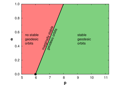
Figure 3: This figure shows the $(p,e)$ parameter space for bound geodesic orbits in Schwarzschild spacetime. The region $p>6\,{+}\,2e$ where stable geodesic orbits are possible is shown in green. In the region shown in red ($p<6\,{+}\,2e$) there are no stable geodesic orbits, only unstable “plunge” ones. The point at $p{=}6$, $e{=}0$ marks the innermost stable circular orbit (ISCO). The line $p=6\,{+}\,2e$ marks the locus of marginally stable orbits, while zoom-whirl orbits are those just to the right of this line.

We normalize $\tau$ (proper time along the particle worldline) to be zero at a (i.e., at some arbitrary) periastron passage $r=r_{\min}$. The particle’s geodesic motion $x^{a}=x^{a}(\tau;p,e)$ can then be computed by integrating an appropriate set of ODEs Sago-2009 , or semi-analytically in terms of elliptic integrals.

III.2 Mode-Sum Regularization

Using the mode-sum regularization discussed in section II.1, Barack and Ori Barack-Ori-2000 , Barack Barack-2001 , and Barack et al. Barack-etal-2002 , have shown that the (Lorenz-gauge) 4-vector gravitational self-force $F^{a}$ at any event along the particle’s worldline is given by

$$F^{a}=\sum_{\ell=0}^{\infty}F^{a\ell}_{\text{reg}}\text{\hskip 5.0pt,}$$ (55)

where the “regularized self-force mode” $F^{a\ell}_{\text{reg}}$ is given by

$$F^{a\ell}_{\text{reg}}=F^{a\ell}_{\text{full},\pm}-\Bigl{(}A^{a}_{\pm}(\ell+\tfrac{1}{2})+B^{a}\Bigr{)}\text{\hskip 5.0pt,}$$ (56)

where the “full self-force mode” $F^{a\ell}_{\text{full},\pm}$ is computed for each $\ell$ as described in section III.3, the $\pm$ refers to two different ways of doing this computation (taking one-sided radial derivatives of the metric perturbation at the particle from either the outside or inside), and $A^{a}_{\pm}$ and $B^{a}$ are “regularization parameters” given semi-analytically in terms of certain elliptic integrals of the orbit parameters. Each full self-force mode $F^{a(\ell)}_{\text{full},\pm}$ is itself finite at the particle, but their sum diverges whereas the regularized sum (55) converges.

The computation of $F^{a(\ell)}_{\text{full},\pm}$ is based on a tensor-spherical-harmonic decomposition of the Lorenz-gauge metric perturbation induced by the particle. Let $g_{ab}$ be the background Schwarzschild metric (used to raise and lower all indices in this section), $g$ be the determinant of $g_{ab}$, $\nabla$ be the corresponding (background) covariant derivative operator, $h_{ab}$ be the physical (retarded) metric perturbation due to the particle, $h=h_{\mu}{}^{\mu}$ be the trace of $h_{ab}$, and $\bar{h}_{ab}=h_{ab}-\tfrac{1}{2}g_{ab}h$ be the trace-reversed metric perturbation. We take $h_{ab}$ to satisfy the Lorenz gauge condition

$$\nabla^{a}\bar{h}_{ab}=0\text{\hskip 5.0pt.}$$ (57)

Let $u^{a}$ be the particle’s 4-velocity.

To first order in $h_{ab}$, the linearized Einstein equations are then

$$\nabla^{c}\nabla_{c}\bar{h}_{ab}+2R^{c}{}_{a}{}^{d}{}_{b}\bar{h}_{cd}=-16\pi T_{ab}\text{\hskip 5.0pt,}$$ (58a)

where

$$T_{ab}=\mu\int_{-\infty}^{\infty}\frac{u_{a}u_{b}\,\delta^{(4)}(x^{c}-x^{c}_{p})}{\sqrt{-g}}\,d\tau$$ (58b)

is the particle’s ($\delta$-function) stress-energy tensor.

Due to the symmetry of the Schwarzschild background, the linearized Einstein equations (58) (together with the added constraint-damping terms discussed in section III.4) are separable into tensorial spherical harmonics via the ansatz

$$\bar{h}_{ab}=\frac{\mu}{r}\sum_{\ell=0}^{\infty}\sum_{m=-\ell}^{+\ell}\sum_{i=1}^{10}a_{\ell}^{(i)}\,\bar{h}^{(i)\ell m}(r,t)\,Y_{ab}^{(i)\ell m}(\theta,\varphi;r)\text{\hskip 5.0pt,}$$ (59)

and similarly for $T_{ab}$.

The resulting separated equations take the form of the coupled linear wave equations

$$\Box\bar{h}^{(i)\ell m}+\sum_{j,a}\mathcal{N}^{(i)\ell}_{(j)a}\partial_{a}\bar{h}^{(j)\ell m}+\sum_{j}\mathcal{M}^{(i)\ell}_{(j)}\bar{h}^{(j)\ell m}=S^{(i)\ell m}\,\delta(r-r_{p})\text{\hskip 5.0pt,}$$ (60)

where $\Box$ is the 2-D scalar wave operator on the Schwarzschild background, and where $\mathcal{N}^{(i)\ell}_{(j)a}$, $\mathcal{M}^{(i)\ell}_{(j)}$, and $S^{(i)\ell m}$ are given analytically as known functions of the indices $(i)$ and/or $(j)$, position, $u^{a}$, and $\ell$ and $m$.

The authors solve the wave equations (60) numerically to obtain the Lorenz-gauge metric perturbation modes $\bar{h}^{(i)\ell m}$ and their gradients along the particle worldline. I describe this numerical solution in section III.4.

III.3 The Full Force Modes

Given the Lorenz-gauge metric perturbation modes $\bar{h}^{(i)\ell m}$ in a neighborhood of the particle worldline, the authors next compute a set of coefficients $f_{(k)\pm}^{a\ell m}$ defined along the particle worldline in terms of (analytically-known) linear combinations of $\bar{h}^{(i)\ell m}$, $\partial_{r\pm}\bar{h}^{(i)\ell m}$, and $\partial_{t\pm}\bar{h}^{(i)\ell m}$, where the $\pm$ corresponds to taking one-sided derivatives from the outside or inside of the particle orbit respectively. (Due to the $\delta$-function source term in the wave equation (60), $\bar{h}^{(i)\ell m}$ is typically $C^{0}$ near the particle, i.e., $\bar{h}^{(i)\ell m}$ is continuous at the particle worldline but its 1st derivatives have a jump discontinuity there.)

Taking into account the tensor spherical harmonic expansion of $\bar{h}_{ab}$ and $T_{ab}$ (as compared to the scalar spherical harmonic expansion implicit in the definition of the $f_{(k)\pm}^{a\ell m}$), the authors then compute

$$F^{a(\ell)}_{\text{full},\pm}=\frac{\mu^{2}}{r_{p}^{2}}\sum_{m=-\ell}^{+\ell}\left(\sum_{p=-3}^{+3}\mathcal{F}_{p\pm}^{a(\ell+p)m}\right)Y^{\ell m}(\theta_{p},\phi_{p})\text{\hskip 5.0pt,}$$ (61)

where each $\mathcal{F}_{p\pm}^{a\ell m}$ is a certain (analytically-known) linear combination of the $f_{(k)\pm}^{a\ell m}$ with the same $\ell$ and $m$. Because of the definition (61) – and more generally because of the decomposition of tensor spherical harmonics into scalar spherical harmonics – a given full force mode $F^{a(\ell)}_{\text{full},\pm}$ depends on the Lorenz-gauge metric perturbation modes $\bar{h}^{(i)\ell^{\prime}m}$ for $\ell{-}3\leq\ell^{\prime}\leq\ell{+}3$.

III.4 Numerical Solution of the Wave Equations (60)

For each $(\ell,m)$ the authors solve the 10 coupled wave equations (60) numerically for the 10 $\bar{h}^{(i)\ell m}$ fields, using 4th order finite differencing on a uniform characteristic (double-null) $(v,u)$ grid.

The authors’ “diamond integral” finite differencing scheme is adapted from those of Lousto-2005 ; Haas-2007 . Since the $\delta$-function source term in the wave equation (60) is nonzero only on the particle’s worldline, grid cells away from the worldline have no source-term contribution, allowing a relatively straightforward finite differencing scheme. The handling of the source term for those grid cells which are intersected by the particle worldline – or where the finite difference molecule is intersected by the particle worldline – is much more complicated, particularly since (for a non-circular orbit) the particle generally crosses grid cells obliquely, with no particular symmetry.

Several other aspects of the numerical solution are worth of note here:

• The authors found that a direct numerical solution of the wave equations (60) was unstable, with rapidly growing violations of the Lorenz gauge constraint (57). Following Barack and Lousto Barack-Lousto-2005 , the authors added constraint-damping terms to the evolution equations so as to dynamically damp these gauge violations.

• The correct initial data for the wave equations (60) isn’t known. Instead, the authors use zero initial data. This results in the evolution initially being dominated by spurious radiation induced by the imperfect initial data. Fortunately, this spurious radiation dies out (radiates away) within a few orbital periods, so in a sufficiently long evolution its influence eventually becomes negligible.

• As always for mode-sum schemes, the numerical calculations are done independently for each $\ell$ and $m$. This makes the calculation trivial to parallelize.

• The length of evolution required (or equivalently, given the authors’ characteristic grid setup, the size of the grid) isn’t known a priori. Rather, the evolution must be long enough (the grid must be large enough) for the initial-data spurious radiation to have decayed to a sufficiently small level and, more generally, for the $\bar{h}^{(i)\ell m}$ field configuration to have reached an equilibrium. In practice, the authors monitor $\bar{h}^{(i)\ell m}$ and its gradient along the particle worldline, and stop the evolution once these become periodic (with the particle-orbit period) to within a numerical error threshold of ${\sim}\,10^{-4}$. If the fields don’t meet this criterion before the evolution ends, the authors increase the size of the grid and rerun the evolution.

III.5 Monopole and Dipole Modes

The authors were unable to obtain stable numerical evolutions of the wave equations (60) for $\ell=0$ or $\ell=1$. Instead, they (Barack, Ori, and Sago Barack-Ori-Sago-2008 ) used a frequency-domain method to solve for $\bar{h}^{(i)\ell m}$ in these cases.

Because $\bar{h}^{(i)\ell m}$ is only $C^{0}$ at the particle worldline ($\bar{h}^{(i)\ell m}$ is continuous at the particle worldline but its 1st derivatives have a jump discontinuity there), a naive frequency-domain method would have very poor convergence due to Gibbs-phenomenon oscillations. The authors (Barack, Ori, and Sago Barack-Ori-Sago-2008 ) have developed an elegant solution to this problem, using the homogeneous modes of the wave equations (60) as a basis for the numerical solution. They report that this “method of extended homogeneous solutions” works very well, with the resulting frequency-domain Fourier sums converging exponentially fast to the desired $\bar{h}^{(i)\ell m}$.

III.6 Conservative and Dissipative Parts of the Self-Force

In general, the technique described in section II.7 for decomposing the self-force into conservative and dissipative parts requires explicitly (numerically) computing the advanced metric perturbation $h^{\text{adv}}_{ab}$ as well as the usual retarded metric perturbation $h^{\text{ret}}_{ab}$. This essentially doubles the overall computational effort.

As an alternative, the authors describe another way of computing the conservative and dissipative parts of the self-force using only the usual (retarded) self-force, assuming only that the particle orbit is periodic with a single intrinsic frequency. (This is the case for the authors’ system of an arbitrary bound geodesic particle orbit in Schwarzschild spacetime, as well as for some types of orbits in Kerr spacetime.) Given this condition, the authors extend an argument of Hinderer and Flanagan Hinderer-Flanagan-2008 to infer that

$$F_{\text{adv}}^{t}(\tau) = -F_{\text{ret}}^{t}(-\tau)$$ (62a)

$$F_{\text{adv}}^{r}(\tau) = +F_{\text{ret}}^{r}(-\tau)$$ (62b)

$$F_{\text{adv}}^{\theta}(\tau) = +F_{\text{ret}}^{\theta}(-\tau)$$ (62c)

$$F_{\text{adv}}^{\varphi}(\tau) = -F_{\text{ret}}^{\varphi}(-\tau)\text{\hskip 5.0pt.}$$ (62d)

Assuming that the usual $F_{\text{ret}}^{a}$ is known for an entire particle orbit, the conservative and dissipative parts of the self-force can then be calculated via (51). As noted in section II.7, this decomposition can also be performed mode-by-mode.

III.7 The $\ell$ Sum

The mode sum (55) is an infinite sum. For computational purposes a finite expression is required. To this end, the authors partition the mode sum, rewriting (55) as

$$F^{a}=\sum_{\ell=0}^{\ell_{\max}}F^{a(\ell)}_{\text{reg}}+\sum_{\ell=\ell_{\max}{+}1}^{\infty}F^{a(\ell)}_{\text{reg}}\text{\hskip 5.0pt,}$$ (63)

where $\ell_{\max}\sim 15$ is a numerical parameter, and compute the first term numerically. (This is the main computation; recall that it requires numerically solving the wave equations (60) for $0\leq\ell\leq\ell_{\max}{+}3$.)

To estimate the second term in the partitioned mode sum (63), the authors consider the conservative and dissipative parts of the self-force separately. For the conservative part, the authors make use of the known large-$\ell$ asymptotic series

$$F^{a(\ell)}_{\text{cons},\text{reg}}=\frac{D_{2}^{a}}{(\ell+\tfrac{1}{2})^{2}}+\frac{D_{4}^{a}}{(\ell+\tfrac{1}{2})^{4}}+\frac{D_{6}^{a}}{(\ell+\tfrac{1}{2})^{6}}+\cdots\text{\hskip 5.0pt,}$$ (64)

where the coefficients $D_{k}^{a}$ don’t depend on $\ell$. The authors least-squares fit the first two terms in this series to the numerically computed values of $F^{a(\ell)}_{\text{cons},\text{reg}}$ for $\ell_{\min}\leq\ell\leq\ell_{\max}$, where $\ell_{\min}\sim 10$ is another numerical parameter. Given the fitted coefficients $\{D_{2}^{a},D_{4}^{a}\}$, the second term of the partitioned mode sum (63) can then be estimated in terms of polygamma functions.

The dissipative part of the mode sum (63) converges much faster (in fact, exponentially fast) and is thus much easier to handle numerically: in practice, $F^{a(\ell)}_{\text{diss},\text{reg}}$ falls below the numerical error even before $\ell=\ell_{\max}$, so the second term in the partitioned mode sum (63) is negligible.

III.8 Results and Discussion

The basic result of the authors’ computations is the 4-vector Lorenz-gauge gravitational self-force $F^{a}$ as a function of time along (around) the particle orbit. Figure 4 shows an example of these results.

Figure 4: This figure shows the self-force components $F^{r}$ (dashed line) and $F^{t}$ (solid line) as a function of scaled Schwarzschild time $t/M$, for a particle orbit with $p=10$ and $e=0.5$ (so that $r_{\min}=6\tfrac{2}{3}M$ and $r_{\max}=20M$). The orbital period is $434M$. Notice the slight asymmetry of the self-force with respect to the orbit (for example, $F^{r}$ peaks slightly after the particle’s periastron passage at $t/M=0$). This is a genuine physical effect, not a numerical artifact.

The authors also studied zoom-whirl orbits, finding and analyzing interesting behavior of the self-force during the whirl phase of the orbit. In the interests of brevity, I won’t discuss this phenomenon here.

The authors have also used their code to make the first calculation of the $\mathcal{O}(\mu)$ self-force corrections to the location and angular frequency of the ISCO Barack-Sago-2009 . This calculation is numerically quite delicate, since the ISCO is a singular point in the $(p,e)$ space of particle orbits (figure 3). The authors used two different techniques to make the calculation, and also made a number of other tests to validate the accuracy of their results. They found that self-force effects shift the ISCO inwards, from $r=6M$ to $\bigl{(}6\,{-}\,3.269\,\mu\bigr{)}M$, and slightly raise its frequency, from $\Omega=1/(6^{3/2}M)$ to $\bigl{(}1\,{+}\,0.4869\,\mu/M\bigr{)}\big{/}(6^{3/2}M)$.

These results are of great interest, both as a benchmark of the current state of the Capra research program and for comparison with other approaches to modelling EMRI dynamics. Notably, they can usefully be compared with post-Newtonian (PN) and effective one-body (EOB) calculations Damour-2010:Schw-grav-self-force-and-EOB ; Barack-Damour-Sago-2010 . As well as providing valuable tests of each formalism, this can help to “calibrate” various undetermined coefficients in the PN and EOB expansions.

IV Accuracy

In trying to model EMRI orbital dynamics and calculate EMRI GW templates, it’s essential to know what accuracy (in the GW phase) is needed, and what accuracy is achievable with various approximation schemes. In this section I briefly discuss these issues.

IV.1 The Accuracy Needed by LISA

Matched filtering of the entire years-long LISA data stream would be impractically expensive for detecting EMRIs with hitherto-unknown parameters (Gair-etal-2004:LISA-EMRI-event-rates, , section 3). However, once EMRIs have been detected by more economical search algorithms Amaro-Seoan-etal-2007:LISA-IMRI-and-EMRI-review ; Porter-2009:LISA-data-analysis-overview , precision modelling and matched filtering of the full LISA data set become practical and even essential to allow detecting and characterizing weaker sources in the presence of strong EMRIs.

The strongest LISA EMRIs may have signal/noise ratios of up to $\rho\sim 100$ after matched filtering Amaro-Seoan-etal-2007:LISA-IMRI-and-EMRI-review ; Porter-2009:LISA-data-analysis-overview , so phase differences on the order of $1/\rho$ radians should be just detectable in matched filtering. If we want the maximum possible science return from the LISA mission, i.e., if we wish to avoid having this science return limited by the finite accuracy of our GW templates, then these templates should have GW phase errors of somewhat less than $10$ milliradians. Any phase errors larger than this run the risk of significantly increasing the overall parameter-estimation error budget. Indeed, if we are lucky and LISA detects a very strong EMRI with (say) $\rho\sim 300$, the allowable GW phase errors may be even smaller, perhaps ${\sim}\,1$–$2$ milliradians.

As a rough approximation, a typical LISA EMRI accumulates ${\sim}\,10^{6}$ radians of orbital phase during its last year of inspiral Amaro-Seoan-etal-2007:LISA-IMRI-and-EMRI-review , so maintaining a phase error of somewhat less than $10$ milliradians implies a fractional error of somewhat less than $10$ parts per billion in the instantaneous GW frequency (whose integral gives the cumulative GW phase), and hence also in the instantaneous EMRI orbital frequency.

It’s non-trivial to translate “required accuracy in the instantaneous EMRI orbital frequency” into “required accuracy in a self-force calculation”, but we can make a crude estimate using the recent analyses of Huerta and Gair (Huerta-Gair-2009, , table 1). As discussed in section II.7, for a quasicircular inspiral they estimated that $\mathcal{O}(\mu^{2})$ self-force effects (an $\mathcal{O}(\mu)\sim 10^{-5}$ fraction of the overall self-force) contribute ${\sim}\,20$ radians to the cumulative GW phase of our typical LISA EMRI. This suggests that a GW phase error tolerance of ${\lesssim}\,10$ milliradians corresponds to a fractional accuracy of roughly

$$\frac{10~{}\text{milliradians}}{20~{}\text{radians}}\times 10^{-5}=5\,{\times}\,10^{-9}$$ (65)

in the overall self-force. This is only a crude estimate, but it does suggest the general order of magnitude of self-force computation accuracy needed to match LISA’s data quality for strong EMRIs.

IV.2 High-Accuracy Capra Computations

How accurate is (will) (can) a Capra-based GW template be? This obviously depends on many factors. Astrophysically, there are a variety of possible perturbations to the vacuum–Einstein-equations (Kerr $+$ compact-object) model used in most Capra calculations to date: magnetic fields, accretion disks Giampieri-1993 ; Chakrabarti-1995 ; Narayan-2000 ; Levin-2006 ; Barausse-Rezzolla-2008 , or even another supermassive BH within a few tenths of a parsec Yunes-Miller-Thornburg-2011 . It remains an open research problem to incorporate such perturbations within Capra models.

Within vacuum–Einstein-equations Capra models, there are two major sources of error in our models of EMRI dynamics and GW emission/propagation:

• Our Capra computational schemes are based on approximations to the Einstein equations. For example, the use of 1st order BH perturbation theory implies fractional errors in self-force effects of at least $\mathcal{O}(\mu)\sim 10^{-5}$ due to neglected 2nd-order effects; 2nd order BH perturbation theory should bring these errors down to $\mathcal{O}(\mu^{2})\sim 10^{-10}$, subject to the long-time-approximation issues discussed in section IV.3 below. No practical 2nd-order Capra computational schemes exist yet; I discuss prospects for their construction in the future in section V.2.

• In practice, we numerically solve our equations using finite-precision arithmetic, and using discrete approximations to the ordinary or partial differential equations (ODEs or PDEs). As discussed in section II.1, frequency-domain methods only require integrating ODEs; these are potentially very accurate. For example, Detweiler, Messaritaki, and Whiting Detweiler-Messaritaki-Whiting-2003 achieved fractional numerical errors ${\lesssim}\,1.5\,{\times}\,10^{-8}$ in a computation of scalar-field self-force acting on a scalar particle in a circular orbit in Schwarzschild spacetime, and Blanchet et al. Blanchet-etal-2010:cmp-3PN-with-self-force achieved fractional numerical errors ${\lesssim}\,10^{-13}$ in a computation of the gravitational self-force for a point mass in a circular orbit in Schwarzschild spacetime. However, time-domain methods require numerically solving PDEs, and have typical fractional numerical accuracies of at best ${\lesssim}\,10^{-4}$, although Thornburg Thornburg-2010:characteristic-AMR ; Thornburg-2011:highly-accurate-self-force achieved fractional accuracies ${\lesssim}\,10^{-6}$ in a time-domain code by combining adaptive mesh refinement with extended-precision floating-point arithmetic.

For very high accuracy all error sources need to be small, i.e., the EMRI’s astrophysical environment must be accurately modelled and the Capra computational scheme must accurately approximate the Einstein equations (probably using 2nd order BH perturbation theory and a long-time approximation of the type described below) and the numerical computations must be very accurate.

IV.3 Long-Time Approximation Schemes

Most Capra research to date has used 1st order BH perturbation theory and taken the small body to move on a fixed (timelike) geodesic worldline in the background Schwarzschild or Kerr spacetime. Assuming some computational scheme for the self-force, an obvious improvement is to use the computed self-force to perturb the particle’s worldline away from being a geodesic, updating a “deviation vector” with the $\mathcal{O}(\mu)$ equations of motion (26). Unfortunately, the worldline is fixed by the 1st-order Bianchi identity, so it’s not obvious that such a scheme can be self-consistent. As very clearly described by Pound Pound-2010a , a “gauge relaxation” technique can be used to allow the particle worldline to vary, but such a scheme can still be valid for at most a short time: since the particle’s orbit gradually shrinks due to GW emission, the particle’s orbital phase differs from that of a reference geodesic by ${\sim}\,1$ radian after the “dephasing time”, which is quite short – $\mathcal{O}(\mu^{-1/2})$. At this point the deviation vector is large, and the whole approximation scheme breaks down.

A much more sophisticated orbital-evolution scheme is needed to avoid this problem, i.e., to remain accurate for the (long) orbital-decay timescales $\mathcal{O}(\mu^{-1})$. Hinderer and Flanagan Hinderer-Flanagan-2008 and Pound Pound-2010a discuss various aspects of how such schemes might be constructed. The detailed definition and implementation of such schemes remains a topic for future research.

V Summary and Future Prospects

V.1 Past Light Cone

A major area of Capra research has long been the effort to analyze the singularity structure of the scalar-field, electromagnetic, and gravitational perturbations induced by point charges/masses. Much of our current understanding of this structure is based on a decomposition due to Detweiler and Whiting Detweiler-Whiting-2003 . As discussed in section II.2, the Detweiler-Whiting decomposition splits the perturbation into a singular part (which is, in a suitable sense, spherically symmetric at the particle) and a “radiative” part which is finite at the particle. In this context it’s common to assume the Detwiler-Whiting postulate, which asserts that by virtue of its symmetry the singular field exerts no force on the particle; self-force effects arise solely from the particle’s interaction with the radiative field. This postulate has recently been rigorously proved by Harte Harte-2006:EM-self-force ; Harte-2008 ; Harte-2009 ; Harte-2010 and Pound Pound-PhD ; Pound-2010a ; Pound-2010b .

A variety of lines of reasoning lead to the (same) “MiSaTaQuWa” equations of motion for the 1st-order-perturbation-theory self-force acting on a small body moving in an external field. The original derivations of these equations are due to Mino, Sasaki, and Tanaka Mino-Sasaki-Tanaka-1997 and Quinn and Wald Quinn-Wald-1997 (thus the name “MiSaTaQuWa”). More recently, the rigorous derivations of Gralla and Wald Gralla-Wald-2008 , Gralla, Harte, and Wald Gralla-Harte-Wald-2009 , and Pound Pound-PhD ; Pound-2010a ; Pound-2010b have helped to put the MiSaTaQuWa equations on a solid mathematical foundation.

The notion of “point particle” has serious foundational difficulties in a nonlinear field theory such as general relativity Geroch-Traschen-1987 (see also footnote 14). However, at least in 1st-order perturbation theory these difficulties seem to be surmountable. As Poisson writes (Poisson-2004-living-review, , section 5.5.4),

The introduction of a point mass in a nonlinear theory of gravitation would appear at first sight to be severely misguided. The lesson learned here is that one can in fact get away with it. The derivation of the MiSaTaQuWa equations of motion based on the method of matched asymptotic expansions does indeed show that results obtained on the basis of a point-particle description can be reliable, in spite of all their questionable aspects. This is a remarkable observation, and one that carries a lot of convenience: It is much easier to implement the point-mass description than to perform the matching of two metrics in two coordinate systems.

The MiSaTaQuWa equations involve a curved-spacetime Green function which can only rarely be explicitly calculated. Instead, almost all practical calculations of self-force effects have returned to the scalar-field, Maxwell, or Einstein equations (as appropriate), and regularized the point-particle singularity.

Barack and Ori Barack-Ori-2000 (see also Barack-2000 ; Barack-2001 ; Barack-etal-2002 ; Barack-Ori-2002 ; Barack-Lousto-2002 ; Barack-Ori-2003 ) developed the “mode-sum” regularization, which provides a practical route to self-force computations. As discussed in section II.1, this scheme first decomposes the field perturbation into spherical harmonics. Each individual spherical-harmonic mode can be calculated by numerically solving a linear wave equation in $1{+}1$ dimensions, or by solving an ODE if a frequency-domain approach is used. The self-force is then obtained by subtracting certain analytically-calculable regularization parameters from the gradient of each mode’s field at the particle, and finally summing over all modes.

The Barack-Ori mode-sum scheme has been the basis for much further research as well as having been used for a large number of self-force calculations in various physical systems. In section III, I summarize a noteworthy recent self-force calculation using this scheme, due to Barack and Sago Barack-Sago-2010 . They calculate the 1st-order-perturbation-theory gravitational self-force acting on a particle in an arbitrary bound geodesic orbit in Schwarzschild spacetime, and find and analyze a variety of interesting physical effects such as the $\mathcal{O}(\mu)$ self-force corrections to the ISCO position and orbital frequency. This marks a major milestone in the Capra research program.

Barack and Golbourn Barack-Golbourn-2007 (see also Barack-Golbourn-Sago-2007 ; Dolan-Barack-2011 ) and Vega and Detweiler Vega-Detweiler-2008:self-force-regularization (see also Vega-etal-2009:self-force-3+1-primer ) have recently developed “puncture-function” regularization schemes. As discussed in section II.6, these schemes first subtract a puncture function (a suitable analytically-calculable approximation to the Detweiler-Whiting singular field) from the physical field near the particle, leaving a finite “residual” field. The Barack-Golbourn “$m$-mode” scheme decomposes the residual field into a Fourier series in the azimuthal ($\varphi$) direction, and calculates each azimuthal mode by numerically solving a linear wave equation in $2{+}1$ dimensions on the Kerr background. The self-force is then obtained by summing the field gradient at the particle over all modes. The Vega-Detweiler scheme numerically solves the regularized field equation (a linear wave equation) for the residual field in $3{+}1$ dimensions, bypassing any mode-sum decomposition. Both the Barack-Golbourn $m$-mode scheme and the Vega-Detweiler scheme are now in use for a variety of self-force calculations.

Because of the complexity of self-force calculations, many techniques have first been developed for scalar-field or electromagnetic particles, and then extended to the gravitational case. Historically, self-force calculations first considered particles moving in Schwarzschild spacetime, but in recent years a growing number of researchers have considered particles in Kerr spacetime.

The self force and its effects can usefully be decomposed into conservative (time-symmetric) and dissipative (time-asymmetric) parts; the latter are often much easier to calculate. It was once thought that accurate EMRI orbital evolutions could be obtained ignoring the conservative part, but Drasco and Hughes Drasco-Hughes-2006 and Pound and Poisson Pound-Poisson-Nickel-2005 ; Pound-Poisson-2008a have found that this isn’t the case. Huerta and Gair Huerta-Gair-2009 have estimated the magnitude of conservative effects as ${\sim}\,20$ radians of GW phase (out of a total accumulated GW phase of ${\sim}\,10^{6}$ radians) during the final year of a typical LISA quasicircular EMRI’s inspiral; conservative effects are likely to be much larger for eccentric inspirals.

V.2 Future Light Cone

Many of the topics discussed in this article remain active areas of research. Some of the areas where I expect to see major developments are:

• Further study of the transient resonance crossings recently identified by Flanagan and Hinderer Flanagan-Hinderer-2010 (described in footnote 23). These could have a major impact on LISA EMRI data analysis.

• Many more self-force calculations for particles orbiting in Kerr spacetime. To this end, several research groups are actively working on implementing and extending the puncture-function computational schemes described in section II.6. Warburton and Barack Warburton-Barack-2010 have also used the “classic” Barack-Ori mode-sum scheme (discussed in section II.1) for Kerr calculations.

• The quantitative comparison of different Capra calculations. Sago, Barack, and Detweiler Sago-Barack-Detweiler-2008 made a very important comparison of this type, showing the consistency of a frequency-domain calculation by Detweiler and a time-domain calculation by Sago and Barack, despite these using different gauges. Such comparisons serve as valuable checks on all the methods and codes involved.

• The use of Capra calculations to help determine free parameters in post-Newtonian approximation schemes, such as the recent work of Blanchet et al. Blanchet-etal-2010:cmp-3PN-with-self-force ; Blanchet-etal-2010:PN-fit-to-Schw-circular-self-force . These comparisons also serve as valuable checks on both the Capra and post-Newtonian schemes and computations.

• The development of improved long-time approximation schemes, initially using simple “orbit perturbation” ideas as described in section IV.2, and later possibly along the lines suggested by Hinderer and Flanagan Hinderer-Flanagan-2008 and/or Pound Pound-2010a (I briefly discuss the need for these in section IV.3).

• The development of analyses, and eventually practical computational schemes, based on 2nd-order BH perturbation theory.^, Pound Pound-2010a has recently reviewed this problem, and has suggested at least one possible route to the construction of a practical 2nd-order scheme. The computations required are likely to be very complicated (both analytically and numerically) but seem to be possible.

• The computation of Capra GW templates, and later the incorporation of many of the other developments mentioned above into the computation of these templates.

The result of these and many other developments will (I hope) eventually be the calculation of highly accurate EMRI orbital dynamics and GW templates. The numerical calculations involved in doing this will almost certainly be very expensive, perhaps comparable or even larger in magnitude to those for a full numerical-relativity simulation of a comparable-mass binary BH inspiral/coalescence/ringdown. Thus it won’t be practical to calculate in this way the huge numbers of GW templates that will be needed for LISA data-analysis template banks. Rather, moderate numbers of Capra GW templates will be used to calibrate other (cheaper) approximation schemes (perhaps $n$th-generation descendents of the “kludge” waveforms used today, or perhaps new schemes like the effective one-body (EOB) ones described by Yunes Yunes-2009:EOB-EMRI-waveforms-review ; Yunes-etal-2010:EOB-EMRI-waveforms ). These cheaper schemes will then be used to generate the actual template banks.

Given the very talented people working on these problems, I predict that Capra EMRI GW templates meeting the accuracy goal described in section IV.2 (${\lesssim}\,10$ milliradians of phase error over a full million-radian inspiral) will be published within 10 years of this article’s appearance. I hope many readers of this article will participate in this effort and that within most of our lifetimes we will see actual LISA data being filtered with these templates. There is much work to do.

- (1) P. Amaro-Seoane, J. R. Gair, M. Freitag, M. C. Miller, I. Mandel, C. J. Cutler, and S. Babak, Class. Quant. Grav. 24, R113 (2007), astro-ph/0703495
- (2) J. R. Gair, Class. Quant. Grav. 26, 094034 (20 April 2009), arXiv:0811.0188
- (3) E. K. Porter, GW Notes 1 (April–June 2009), ISSN 1868-1921, arXiv:0910.0373
- (4) T. Damour, in Three Hundred Years of Gravitation, edited by S. W. Hawking and W. Israel (Cambridge University Press, Cambridge, England, 1987) Chap. 6, pp. 128–198, ISBN 0-521-34312-7
- (5) L. Blanchet, Living Reviews in Relativity 9 (2006), http://www.livingreviews.org/lrr-2006-4
- (6) T. Futamase and Y. Itoh, Living Reviews in Relativity 10 (2007), http://www.livingreviews.org/lrr-2007-2
- (7) L. Blanchet, in Mass and Motion in General Relativity, edited by L. Blanchet, A. Spallicci, and B. F. Whiting (Springer-Verlag, Berlin, 2010) ISBN 978-90-481-3014-6, arXiv:0907.3596
- (8) G. Schäfer, in Mass and Motion in General Relativity, edited by L. Blanchet, A. Spallicci, and B. F. Whiting (Springer-Verlag, Berlin, 2010) ISBN 978-90-481-3014-6, arXiv:0910.2857
- (9) F. Pretorius, in Relativistic Objects in Compact Binaries: From Birth to Coalescence, edited by M. Colpi (Springer-Verlag, 2007) arXiv:0710.1338
- (10) M. Hannam, S. Husa, J. G. Baker, M. Boyle, B. Brügmann, T. Chu, N. Dorband, F. Herrmann, I. Hinder, B. J. Kelly, L. E. Kidder, P. Laguna, K. D. Matthews, J. R. van Meter, H. P. Pfeiffer, D. Pollney, C. Reisswig, M. A. Scheel, and D. Shoemaker, Phys. Rev. D 79, 084025 (2009), arXiv:0901.2437
- (11) M. Hannam, Class. Quant. Grav. 26, 114001 (2009), arXiv:0901.2931
- (12) M. Hannam and I. Hawke, General Relativity and Gravitation 43, 465 (2010), arXiv:0908.3139
- (13) I. Hinder, Class. Quant. Grav. 27, 114004 (2010), arXiv:1001.5161
- (14) M. Campanelli, C. O. Lousto, B. C. Mundim, H. Nakano, Y. Zlochower, and H.-P. Bischof, Classical and Quantum Gravity 27, 084034 (2010), arXiv:1001.3834
- (15) J. M. Centrella, J. G. Baker, B. J. Kelly, and J. R. van Meter, Rev. Mod. Phys. 82, 3069 (Nov 2010), arXiv:1010.5260
- (16) C. O. Lousto and Y. Zlochower, Phys. Rev. Lett. 106, 041101 (Jan 2011), arXiv:1009.0292
- (17) N. T. Bishop, R. Gómez, S. Husa, L. Lehner, and J. Winicour, Phys. Rev. D 68, 084015 (Oct 2003), gr-qc/0301060
- (18) N. T. Bishop, R. Gómez, L. Lehner, M. Maharaj, and J. Winicour, Phys. Rev. D 72, 024002 (Jul 2005), gr-qc/0412080
- (19) C. F. Sopuerta, P. Sun, P. Laguna, and J. Xu, Class. Quant. Grav. 23, 251 (2006), gr-qc/0507112
- (20) C. F. Sopuerta and P. Laguna, Phys. Rev. D 73, 044028 (Feb 2006), gr-qc/0512028
- (21) C. O. Lousto, H. Nakano, Y. Zlochower, and M. Campanelli, Phys. Rev. Lett. 104, 211101 (May 2010), arXiv:1001.2316
- (22) C. W. Misner, K. S. Thorne, and J. A. Wheeler, Gravitation (W. H. Freeman, San Francisco, 1973) ISBN 0-7167-0334-3 (hc), 0-7167-0344-0 (paper)
- (23) E. Poisson, Living Reviews in Relativity 7 (2004), http://www.livingreviews.org/lrr-2004-6
- (24) E. Poisson, in General Relativity and Gravitation: Proceedings of the 17th International Conference, Dublin, 18–23 July 2004, edited by P. Florides, B. Nolan, and A. Ottewill (World Scientific, New Jersey, USA, 2005) pp. 119–141, ISBN 981-256-424-1, gr-qc/0410127
- (25) E. Poisson, in Mass and Motion in General Relativity, edited by L. Blanchet, A. Spallicci, and B. F. Whiting (Springer-Verlag, Berlin, 2010) ISBN 978-90-481-3014-6, arXiv:0909.2994
- (26) S. Detweiler, Class. Quant. Grav. 22, S681 (7 August 2005), gr-qc/0501004
- (27) L. Barack, Class. Quant. Grav. 26, 213001 (2009), arXiv:0908.1664
- (28) J. Thornburg, “Web site of the 2009 Capra meeting, held 15–19 June, 2009, in Bloomington, Indiana, USA,” (2009), http://www.astro.indiana.edu/~jthorn/capra12/capra12.html
- (29) L. Lehner, H. Pfeiffer, and E. Poisson, “Web site of the 2010 Capra/NRDA meetings, held 20–26 June, 2010, in Waterloo, Ontario, Canada,” (2010), http://www.perimeterinstitute.ca/Events/Theory_Meets_Data_Analysis/Sch%****␣capra-survey.bbl␣Line␣425␣****edule/
- (30) N. Sago, L. Barack, and S. Detweiler, Phys. Rev. D 78, 124024 (2008), arXiv:0810.2530
- (31) R. Geroch and J. Traschen, Phys. Rev. D 36, 1017 (Aug 1987)
- (32) L. Barack and A. Ori, Phys. Rev. D 64, 124003 (Oct 2001), gr-qc/0107056
- (33) L. Barack and N. Sago, Phys. Rev. D 81, 084021 (Apr 2010), arXiv:1002.2386
- (34) Y. Mino, M. Sasaki, and T. Tanaka, Phys. Rev. D 55, 3457 (Mar 1997), gr-qc/9606018
- (35) T. C. Quinn and R. M. Wald, Phys. Rev. D 56, 3381 (1997), gr-qc/9610053
- (36) L. Barack and A. Ori, Phys. Rev. D 61, 061502(R) (Feb 2000), gr-qc/9912010
- (37) S. Detweiler and B. F. Whiting, Phys. Rev. D 67, 024025 (Jan 2003), gr-qc/0202086
- (38) L. Barack and D. A. Golbourn, Phys. Rev. D 76, 044020 (Aug 2007), arXiv:0705.3620
- (39) L. Barack, D. A. Golbourn, and N. Sago, Phys. Rev. D 76, 124036 (2007), arXiv:0709.4588
- (40) S. R. Dolan and L. Barack, Phys. Rev. D 83, 024019 (Jan 2011), arXiv:1010.5255
- (41) I. Vega and S. Detweiler, Phys. Rev. D 77, 084008 (Apr 2008), arXiv:0712.4405
- (42) I. Vega, P. Diener, W. Tichy, and S. Detweiler, Phys. Rev. D 80, 084021 (Oct 2009), arXiv:0908.2138
- (43) A. Ori, Physics Letters A 202, 347 (1995), gr-qc/9507048
- (44) A. Ori, Phys. Rev. D 55, 3444 (Mar 1997)
- (45) L. Barack, Phys. Rev. D 62, 084027 (Sep 2000), gr-qc/0005042
- (46) L. Barack, Phys. Rev. D 64, 084021 (Sep 2001), gr-qc/0105040
- (47) L. Barack, Y. Mino, H. Nakano, A. Ori, and M. Sasaki, Phys. Rev. Lett. 88, 091101 (4 March 2002), gr-qc/0111001
- (48) L. Barack and A. Ori, Phys. Rev. D 66, 084022 (2002), gr-qc/0204093
- (49) L. Barack and C. O. Lousto, Phys. Rev. D 66, 061502(R) (2002), gr-qc/0205043
- (50) L. Barack and A. Ori, Phys. Rev. D 67, 024029 (2003), gr-qc/0209072
- (51) L. Barack and A. Ori, Phys. Rev. Lett. 90, 111101 (Mar 2003), gr-qc/0212103
- (52) S. Detweiler, E. Messaritaki, and B. F. Whiting, Phys. Rev. D 67, 104016 (May 2003), gr-qc/0205079
- (53) P. A. M. Dirac, Proceedings of the Royal Society of London, A 167, 148 (1938)
- (54) B. S. DeWitt and R. W. Brehme, Annals of Physics 9, 220 (February 1960)
- (55) J. M. Hobbs, Annals of Physics 47, 141 (March 1968)
- (56) A. I. Harte, Phys. Rev. D 73, 065006 (Mar 2006), gr-qc/0508123
- (57) A. I. Harte, Classical and Quantum Gravity 25, 235020 (Dec 2008), arXiv:0807.1150
- (58) A. I. Harte, Classical and Quantum Gravity 26, 155015 (Aug 2009), arXiv:0903.0167
- (59) A. I. Harte, Classical and Quantum Gravity 27, 135002 (Jul 2009), arXiv:0910.4614
- (60) A. Pound, Motion of Small Bodies in General Relativity: Foundations and Implementations of the Self-Force, Ph.D. thesis, University of Guelph, Guelph, Canada (2010), arXiv:1006.3903
- (61) A. Pound, Phys. Rev. D 81, 024023 (Jan 2010), arXiv:0907.5197
- (62) A. Pound, Phys. Rev. D 81, 124009 (Jun 2010), arXiv:1003.3954
- (63) R. Steinbauer and J. A. Vickers, Classical and Quantum Gravity 23, R91 (2006), gr-qc/0603078v2
- (64) S. E. Gralla, A. I. Harte, and R. M. Wald, Phys. Rev. D 80, 024031 (July 2009), arXiv:0905.2391
- (65) S. E. Gralla and R. M. Wald, Class. Quant. Grav. 25, 205009 (21 October 2008), arXiv:0806.3293
- (66) B. Wardell, Green Functions and Radiation Reaction From a Spacetime Perspective, Ph.D. thesis, University College Dublin, Dublin (2009), arXiv:0910.2634
- (67) A. C. Ottewill and B. Wardell, Phys. Rev. D 77, 104002 (May 2008), arXiv:0711.2469
- (68) A. C. Ottewill and B. Wardell, Phys. Rev. D 79, 024031 (Jan 2009), arXiv:0810.1961
- (69) A. C. Ottewill and B. Wardell, “A transport equation approach to calculations of Green functions and HaMiDeW coefficients,” (2009), arXiv:0906.0005
- (70) B. Wardell and I. Vega, “A generic effective source for scalar self-force calculations,” (2011), manuscript in preparation
- (71) I. Vega, B. Wardell, and P. Diener, “Effective source approach to self-force calculation,” (2011), arXiv:1101.2925
- (72) P. Cañizares and C. F. Sopuerta, J. Physics: Conference Series 159, 012053 (2009), proceedings of the 7th International LISA Symposium, Barcelona, Spain, 16–20 June 2008, arXiv:0811.0294
- (73) P. Cañizares and C. F. Sopuerta, Phys. Rev. D 79, 084020 (Apr 2009), arXiv:0903.0505
- (74) Y. Mino, Phys. Rev. D 67, 084027 (Apr 2003), gr-qc/0302075
- (75) Y. Mino, Classical and Quantum Gravity 22, S717 (2005), gr-qc/0506002
- (76) Y. Mino, Progress of Theoretical Physics 113, 733 (2005), gr-qc/0506003
- (77) Y. Mino, Progress of Theoretical Physics 115, 43 (2006), arXiv:gr-qc/0601019
- (78) Y. Mino, Phys. Rev. D 77, 044008 (Feb 2008), arXiv:0711.3007
- (79) S. Drasco and S. A. Hughes, Phys. Rev. D 73, 024027 (Jan 2006), gr-qc/0509101
- (80) A. Pound, E. Poisson, and B. G. Nickel, Phys. Rev. D 72, 124001 (Dec 2005), gr-qc/0509122
- (81) A. Pound and E. Poisson, Phys. Rev. D 77, 044012 (Feb 2008), arXiv:0708.3037
- (82) E. A. Huerta and J. R. Gair, Phys. Rev. D 79, 084021 (2009)
- (83) L. Barack and N. Sago, “Beyond the geodesic approximation: conservative effects of the gravitational self-force in eccentric orbits around a Schwarzschild black hole,” (2011), arXiv:1101.3331
- (84) N. Sago, Class. Quant. Grav. 26, 094025 (2009)
- (85) C. O. Lousto, Class. Quant. Grav. 22, S543 (2005), gr-qc/0503001
- (86) R. Haas, Phys. Rev. D 75, 124011 (Jun 2007), arXiv:0704.0797
- (87) L. Barack and C. O. Lousto, Phys. Rev. D 72, 104026 (2005), gr-qc/0510019
- (88) S. E. Field, J. S. Hesthaven, and S. R. Lau, Phys. Rev. D 81, 124030 (Jun 2010), arXiv:1001.2578
- (89) J. L. Jaramillo, C. F. Sopuerta, and P. Canizares, “Are time-domain self-force calculations contaminated by Jost solutions?.” (2011), arXiv:1101.2324
- (90) J. Thornburg, General Relativity and Gravitation in press (2010), doi:“bibinfo–doi˝–10.1007/s10714-010-1096-z˝, arXiv:0909.0036
- (91) J. Thornburg, “Highly accurate and efficient self-force computation using time-domain methods: Error estimates, validation, and optimization,” (2010), arXiv:1006.3788
- (92) L. Barack, A. Ori, and N. Sago, Phys. Rev. D 78, 084021 (2008), arXiv:0808.2315
- (93) T. Hinderer and E. E. Flanagan, Phys. Rev. D 78, 064028 (2008), arXiv:0805.3337
- (94) L. Barack and N. Sago, Phys. Rev. Lett. 102, 191101 (2009), arXiv:0902.0573
- (95) T. Damour, Phys. Rev. D 81, 024017 (2010), arXiv:0910.5533
- (96) L. Barack, T. Damour, and N. Sago, Phys. Rev. D 82, 084036 (2010), arXiv:1008.0935
- (97) J. R. Gair, L. Barack, T. Creighton, C. Cutler, S. L. Larson, E. S. Phinney, and M. Vallisneri, Class. Quant. Grav. 21, S1595 (2004), gr-qc/0405137
- (98) Éanna É. Flanagan and T. Hinderer, “Transient resonances in the inspirals of point particles into black holes,” (2010), arXiv:1009.4923
- (99) G. Giampieri, “Sinusoidal gravitational waves from the nuclei of active galaxies,” (1993), astro-ph/9305034
- (100) S. K. Chakrabarti, Phys. Rev. D 53, 2901 (Mar 1996), astro-ph/9603117
- (101) R. Narayan, The Astrophysical Journal 536, 663 (jun 2000), astro-ph/9907328
- (102) Y. Levin, Mon. Not. Roy. Astron. Soc. 374, 515 (Jan 2007), astro-ph/0603583
- (103) E. Barausse and L. Rezzolla, Phys. Rev. D 77, 104027 (May 2008), 0711.4558
- (104) N. Yunes, M. C. Miller, and J. Thornburg, Phys. Rev. D in press (2011), arXiv:1010.1721
- (105) L. Blanchet, S. Detweiler, A. Le Tiec, and B. F. Whiting, Phys. Rev. D 81, 064004 (Mar 2010), arXiv:0910.0207
- (106) N. Warburton and L. Barack, Phys. Rev. D 81, 084039 (Apr 2010), arXiv:1003.1860
- (107) L. Blanchet, S. Detweiler, A. Le Tiec, and B. F. Whiting, Phys. Rev. D 81, 084033 (Apr 2010), arXiv:1002.0726
- (108) E. Rosenthal, Class. Quant. Grav. 22, S859 (7 August 2005), gr-qc/0501046
- (109) E. Rosenthal, Phys. Rev. D 72, 121503(R) (2005), gr-qc/0508050
- (110) E. Rosenthal, Phys. Rev. D 73, 044034 (2006), gr-qc/0602066
- (111) E. Rosenthal, Phys. Rev. D 74, 084018 (2006), gr-qc/0609069
- (112) L. Barack and C. Cutler, Phys. Rev. D 69, 082005 (2004), gr-qc/0310125
- (113) S. Babak, H. Fang, J. R. Gair, K. Glampedakis, and S. A. Hughes, Phys. Rev. D 75, 024005 (2007), gr-qc/0607007
- (114) S. Babak, H. Fang, J. R. Gair, K. Glampedakis, and S. A. Hughes, Phys. Rev. D 77, 049902 (2008), gr-qc/0607007
- (115) N. Yunes, GW Notes 2 (July–September 2009), ISSN 1868-1921
- (116) N. Yunes, A. Buonanno, S. A. Hughes, M. C. Miller, and Y. Pan, Phys. Rev. Lett. 104, 091102 (Mar 2010), arXiv:0909.4263