Fluctuations of the number of participants and binary collisions
in AA-interactions at fixed centrality in Glauber approach

V. V. Vechernin and H. S. Nguyen


Department of High-Energy Physics, St. Petersburg State University,
RU-198504 St. Petersburg, Russia
{\dagger}
E-mail: vechernin@pobox.spbu.ru


Abstract

In the framework of classical Glauber approach the analytical expressions for the variance of the number of wounded nucleons and binary collisions in AA interactions at given centrality are presented. Along with the optical approximation term they contain the additional contact terms, arising only in the case of nucleus-nucleus collisions. The magnitude of the additional contributions, e.g. for PbPb collisions at SPS energies, at some values of the impact parameter is larger than the contribution of the optical approximation, with their sum being in a good agreement with the results of independent Monte-Carlo simulations of this process. Due to these additional terms the variance of the total number of participants for peripheral PbPb collisions and the variance of the number of collisions at all values of the impact parameter exceed several times the Poisson ones. The correlator between the numbers of participants in colliding nuclei at fixed centrality is also analytically calculated.


1 Introduction

At present the considerable attention is devoted to the experimental and theoretical investigations of the multiplicity and transverse momentum fluctuations of charged particles in high energy AA collisions (see [1]-[7] and references therein). One expects the increase of the fluctuations in the case of freeze-out close to the QCD critical endpoint of the quark-gluon plasma - hadronic matter phase boundary line [8, 9].

The aim of the present paper is to draw an attention to another factor leading to the increase of the fluctuations in the case of AA interactions. Namely the increase of the fluctuations of the number of participants and binary collisions due to multiple contact nucleon interactions in nucleus-nucleus collisions.

Clear that these fluctuations lead to fluctuations in the number of particle sources and so directly impact on the multiplicity and transverse momentum fluctuations of produced charged particles and also on the correlations between them (see, for example, [10]-[17]).

In the present paper the analytical expressions for the variance of the number of wounded nucleons and binary collisions in given centrality AA interactions are obtained taking into account the multiple contact NN interactions (so-called loop contributions). The calculations are fulfilled in the framework of classical Glauber approach [18], having a simple probabilistic interpretation [19, 20]. In contrast with purely Monte-Carlo simulations the analytical calculations enable to understand the origin of increased values of the fluctuations.

As a result we demonstrate that the multiple contact NN interactions in AA scattering lead in particular to the fact that, e.g. for PbPb collisions at SPS energies, the variance of the total number of participants for peripheral collisions and the variance of the number of collisions at all values of the impact parameter exceed a few times the Poisson ones.

The paper is organized as follows. In section 2 in the framework of classical Glauber approach we present the analytical expression for the variance of the number of wounded nucleons in one of the colliding nucleus at a fixed value of the impact parameter. Along with the well known optical contribution (which depends only on the total inelastic NN cross-section) in the case of nucleus-nucleus collisions there is the additional contact term, depending on the profile of the NN interaction probability in the impact parameter plane.

In section 3 we calculate the correlator between the numbers of participants in colliding nuclei at fixed centrality and as a consequence find the variance of the total (in both nuclei) number of participants.

In section 4 in the framework of the same approach we present the analytical expression for the variance of the number of NN binary collisions in given centrality AA interactions. Along with the optical approximation term it also contains other terms, which occur the dominant ones. These terms also correspond to the multinucleon contact interactions and arise only in the case of nucleus-nucleus collisions.

The derivations of all formulas are taken into the appendices A, B and C.

All over the paper the results of numerical calculations are presented with the purpose to illustrate the obtained analytical results. We control also the results of our analytical calculations comparing them with the results obtained by purely Monte-Carlo simulations of the nucleus-nucleus scattering.

Note that we restrict our consideration by the region of the impact parameter $\beta<R_{A}+R_{B}$, where the probability of inelastic interaction $\sigma_{\!AB}(\beta)$ of two nuclei with radii $R_{A}$ and $R_{B}$ is close to unity.

2 Variance of the participants number in one nucleus

At first we consider the variance $V[N^{A}_{w}(\beta)]$ of the number of participants $N^{A}_{w}(\beta)$ (wounded nucleons) at a fixed value of the impact parameter $\beta$ in one of the colliding nuclei $A$. In the framework of pure classical, probabilistic approach to nucleus-nucleus collisions, formulated in [18], we find for the mean value and for the variance of $N^{A}_{w}(\beta)$ the following expressions (see appendix A):

$$\langle N^{A}_{w}(\beta)\rangle=AP(\beta)\ ,$$ (1)
$$V[N^{A}_{w}(\beta)]=AP(\beta)Q(\beta)+A(A-1)[Q^{(12)}(\beta)-Q^{2}(\beta)]\ ,$$ (2)

where $P(\beta)=1-Q(\beta)$. For $Q(\beta)$ and $Q^{(12)}(\beta)$ we have (all integrations imply the integration over two-dimensional vectors in the impact parameter plane):

$$Q(\beta)=\int da\ T_{A}(a)[1-f_{B}(a\!+\!\beta)]^{B}\ ,$$ (3)
$$Q^{(12)}(\beta)=\int da_{1}da_{2}T_{A}(a_{1})T_{A}(a_{2})[1-f_{B}(a_{1}\!+\!\beta)-f_{B}(a_{2}\!+\!\beta)+g_{B}(a_{1}\!+\!\beta,a_{2}\!+\!\beta)]^{B}$$ (4)

with

$$f_{B}(a)\equiv\int db\ T_{B}(b)\sigma(a\!-\!b)\ ,$$ (5)
$$g_{B}(a_{1},a_{2})\equiv\int db\ T_{B}(b)\sigma(a_{1}\!-\!b)\sigma(a_{2}\!-\!b)\ .$$ (6)

Here $T_{A}$ and $T_{B}$ are the profile functions of the colliding nuclei $A$ and $B$. The $\sigma(a)$ is the probability of inelastic interaction of two nucleons at the impact parameter $a$. We’ll imply that $\sigma(a)$, $T_{A}$ and $T_{B}$ depend only on the magnitude of their two-dimensional vector argument. Hence $f_{B}(a)=f_{B}(|a|)$ and $Q(\beta)=Q(|\beta|)$.

The formula (1) and the first term in formula (2) correspond to the naive picture (so-called optical approximation) implying that in the case of AA-collision at the impact parameter $\beta$ one can use the binomial distribution for $N^{A}_{w}(\beta)$ (see, for example, [21, 22]):

$$\wp_{opt}(N^{A}_{w})=C^{N^{A}_{w}}_{A}\,P(\beta)^{N^{A}_{w}}\,Q(\beta)^{A-N^{A}_{w}},\hskip 28.45274ptP(\beta)=1-Q(\beta)$$ (7)

with some averaged probability $P(\beta)$ of inelastic interaction of a nucleon of the nucleus $A$ with nucleons of the nucleus $B$. At that the $P(\beta)$ is considered to be the same for all nucleons of the nucleus $A$. In the optical approximation one has

$$\langle N^{A}_{w}(\beta)\rangle_{opt}=AP(\beta)\ ,\hskip 28.45274ptV[N^{A}_{w}(\beta)]_{opt}=AP(\beta)Q(\beta)\ .$$ (8)

The whole expression (2) for the variance is the result of more accurate calculation (see appendix A), when at first one calculates the probabilities of all binary NN-interactions, taking into account the impact parameter plane positions of nucleons in the nuclei $A$ and $B$ and only then averages over nucleon positions:

$$V[N^{A}_{w}(\beta)]=\langle{N_{w}^{A}(\beta)}^{2}\rangle-\langle N^{A}_{w}(\beta)\rangle^{2}\ ,$$ (9)

where

$$\langle X\rangle\equiv\langle\langle\overline{X}\rangle_{B}\rangle_{A}\equiv\int\overline{X}\prod_{{k}=1}^{B}T_{B}(b_{k})db_{k}\prod_{{j}=1}^{A}T_{A}(a_{j})da_{j}\ .$$ (10)

Here $\overline{X}$ is the average value of some variate $X$ at fixed positions of all nucleons in the nuclei $A$ and $B$; $\langle{\ }\rangle_{A}$ and $\langle{\ }\rangle_{B}$ denote averaging over positions of these nucleons with corresponding nuclear profile functions.

In the limit $r_{N}\ll R_{A},R_{B}$ the formulae (5) and (6) reduce to

$$f_{B}(a)\approx\sigma_{\!N\!N}\,T_{B}(a)\ ,\hskip 28.45274ptg_{B}(a_{1},a_{2})\approx I(a_{1}-a_{2})\cdot T_{B}((a_{1}+a_{2})/2)$$ (11)

with

$$\sigma_{\!N\!N}\equiv\int\!db\,\sigma(b)\ ,\hskip 71.13188ptI(a)\equiv\int db\,\sigma(b)\,\sigma(b+a)\ .$$ (12)

Note that in this limit the $Q(\beta)$ and hence the mean value (1) and the first term of the variance (2) depend only on the integral inelastic $N\!N$ cross-section $\sigma_{\!N\!N}$, but the $Q^{(12)}(\beta)$ entering the second term of the variance (2) depends also on the shape of the function $\sigma(b)$ through the integral $I(a)$ (12).

Note also that using of the simple approximation with the $\delta$-function: $\sigma(b)=\sigma_{\!N\!N}\delta(b)$ for $N\!N$ interaction gives the same result (as going to the limit $r_{N}\ll R_{A},R_{B}$) only for the optical part of the answer, which is expressed through $Q(\beta)$. If someone tries to use the approximation $\sigma(b)=\sigma_{\!N\!N}\delta(b)$ to calculate $Q^{(12)}(\beta)$, he will get $I(a)=\sigma_{\!N\!N}^{2}\delta(a)$ and $g_{B}=\sigma_{\!N\!N}^{2}\delta(a_{1}-a_{2})\cdot T_{B}(a_{1})$, what leads to infinite $Q^{(12)}(\beta)$ at $B\geq 2$. Meanwhile, for any correct approximation of $\sigma(b)$ with $\sigma(b)\leq 1$ (in correspondence with its probabilistic interpretation in classical Glauber approach) we find a finite answer for $Q^{(12)}(\beta)$.

In the quantum case in Glauber approximation due to unitarity one has

$$\sigma(b)\equiv{\sigma^{in}}(b)={\sigma^{tot}}(b)-{\sigma^{el}}(b)=2{\,\rm{Im}\,}\gamma(b)-|\gamma(b)|^{2}\geq 0\ ,$$ (13)

where the $\gamma(b)$ is the amplitude of $N\!N$ elastic scattering. This leads to the restrictions: $0\leq{\sigma^{tot}}(b)\leq 4$,  $0\leq{\sigma^{el}}(b)\leq 4$ and $0\leq{\sigma^{in}}(b)\leq 1$. So in the quantum case the $\sigma(b)$ also admits a probabilistic interpretation [19, 20].

In our numerical calculations we have used for $\sigma(b)$ the ”black disk” approximation:

$$\sigma(b)=\theta(r_{N}-|b|)\ ,$$ (14)

and Gauss approximation:

$$\sigma(b)=\exp(-b^{2}/r^{2}_{N})\ .$$ (15)

In both cases $\sigma_{\!N\!N}=\pi r^{2}_{N}$. For the nuclear profile functions $T_{A}$ and $T_{B}$ we have used the standard Woods-Saxon approximation:

$$T_{A}(a)=\int\!dz\,\rho(r)\ ,\hskip 28.45274ptr^{2}=a^{2}+z^{2}\ ,\hskip 28.45274pt\rho(r)=\rho_{0}\left(1+\exp\frac{r-R_{A}}{\kappa}\right)^{-1}$$ (16)

with $R_{A}=R_{0}A^{\frac{1}{3}}$, $R_{0}$=1.07 fm, $\kappa$=0.545 fm and $\rho_{0}$ fixed by the condition $\int\!da\,T_{A}(a)\!=\!1$.

Refer to caption

Figure 1: The variance of the number of wounded nucleons in one nucleus for PbPb collisions at SPS energies ($\sigma_{\!N\!N}$=31 mb) as a function of the impact parameter $\beta$ (fm). The points $\bullet$ and   - results of numerical calculations by the analytical formulae (2)–(4), (11) and (12) using respectively the black disk (14) and Gaussian (15) approximations for $N\!N$ interaction;  $\circ$ and - results of independent MC simulations using for $N\!N$ interaction the black disk (14) or Gaussian (15) approximation;  ${\ast}$ - the optical approximation result (8) (the first term in formula (2));  + - the Poisson variance: $V[N^{A}_{w}(\beta)]=\langle N^{A}_{w}(\beta)\rangle$. The curves are shown to guide eyes.

The numerical evaluation of the contribution of the additional (contact) term in formula (2) one can see in Fig.1 presented as an example for PbPb collisions at SPS energies ($r_{N}$=1 fm, $\sigma_{\!N\!N}$=31 mb). For the control we have also carried out independent calculations of the mean values and the variances involved by MC simulations of the AA scattering presenting the results on the same figures.

In Fig.1 we see that the contact term in (2) is essential and gives approximately the same contribution to the variance of the $N^{A}_{w}(\beta)$ in PbPb collisions at intermediate and large values of $\beta$ as the first optical term. It’s important that as we see in Fig.1 the results of independent MC simulations of the $N^{A}_{w}(\beta)$ variance are in a good agreement with the results of the analytical calculations by formula (2) only if one takes into account the contact term.

We see also in Fig.1 that for peripheral AA collisions at large $\beta$, when $P(\beta)$ becomes small ($P(\beta)\ll$1, $Q(\beta)\approx 1$), the optical approximation (7) reduces to the Poisson distribution with $V[N^{A}_{w}(\beta)]_{opt}\approx\langle N^{A}_{w}(\beta)\rangle$ (8).

So only due to the contact term the variance of the $N^{A}_{w}(\beta)$ is larger than the Poisson one for peripheral PbPb collisions (at $\beta>7$ fm) in a correspondence with the indications, which one has from the experimental data on the dependence of multiplicity fluctuations on the centrality at SPS and RHIC energies [1, 4].

The week dependence of the results on the form of $N\!N$ interaction at nucleon distances is also seen. In the case of using the black disk (14) approximation for $\sigma(b)$ the results lay systematically slightly higher, than in the case of using the Gaussian (15) approximation with the same value of $\sigma_{\!N\!N}$.

In Fig.2 we see that the mean value $\langle N^{A}_{w}(\beta)\rangle$ (1), in contrast to the variance, coincides with the optical approximation result (8) and depends only on $\sigma_{\!N\!N}$ in the limit $r_{N}\ll R_{A},R_{B}$. The MC simulations also confirm this result.

Refer to caption

Figure 2: The same as in Fig.1, but for the mean number of wounded nucleons in one nucleus, calculated by formulae (1), (3), (5) and by independent MC simulations; ${\ast}$ - the optical approximation result, calculated using formulae (1), (3) and (12).

We would like to emphasize that the nontrivial term in the expression (2) for the variance arises only in the case of nucleus-nucleus collisions. At $A=1$ or $B=1$ it vanishes. At $A=1$ due to explicit factor $A-1$ in (2) and at $B=1$ due to fact that in this case $Q^{(12)}(\beta)=Q^{2}(\beta)$. This corresponds to the well known fact that for nucleus-nucleus collisions the Glauber approach doesn’t reduce to the optical approximation even in the limit $r_{N}\ll R_{A},R_{B}$ (see, for example, [23]).

The additional term, which arises in the expression for the variance (2) in the case of nucleus-nucleus collisions, depends, as we have mentioned, not only on the integral value of inelastic NN𝑁𝑁N\!N cross-section σNN=𝑑bσ(b)subscript𝜎𝑁𝑁differential-d𝑏𝜎𝑏\sigma_{\!N\!N}=\int\!db\,\sigma\!(b), but also on the shape of the function σ(b)𝜎𝑏\sigma(b), i.e. on the details of NN𝑁𝑁N\!N interaction at nucleon distances, which are much smaller than the typical nuclear distances. 
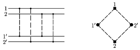
In quantum Glauber approach it corresponds to the fact that in the case of AA collisions, in contrast with pA collisions, the loop diagrams of the type shown in Fig.3 appear and one encounters the contact terms problem (see, for example, [23, 24, 25]).

Refer to caption

Figure 3: An example of the loop diagram in AA-collisions. 1 and 2 - nucleons of the nucleus A;  $1^{\prime}$ and $2^{\prime}$ - nucleons of the nucleus B (see [23, 24, 25] for details).

The second term in formula (2) is the manifestation of this problem at the classical level. In the case of a tree diagram the ”lengths” of the interaction links in the transverse plane are independent. As a consequence the result expresses only through $P(\beta)$ - the probability of the interaction of a nucleon of the nucleus $A$ with nucleons of the nucleus $B$ averaged over its position in nucleus $A$. The $P(\beta)$ is the same for any nucleon of the nucleus $A$. In the case of the loop diagram in Fig.3 the ”lengths” of the interaction links in the transverse plane are not independent and the result can’t be expressed only through the averaged probability $P(\beta)$ and the correlation effects have to be taken into account.

3 Variance of the total number of participants

Now we pass to the calculation of the variance of the total number of participants $V[N^{A}_{w}(\beta)+N^{B}_{w}(\beta)]$ at a fixed value of the impact parameter $\beta$. Clear, that for the mean value we have simply:

$$\langle N^{A}_{w}(\beta)+N^{B}_{w}(\beta)\rangle=\langle N^{A}_{w}(\beta)\rangle+\langle N^{B}_{w}(\beta)\rangle$$ (17)

and by (9) for the variance

$$V[N^{A}_{w}(\beta)+N^{B}_{w}(\beta)]=V[N^{A}_{w}(\beta)]+V[N^{B}_{w}(\beta)]+2\{\langle N_{w}^{A}(\beta)N^{B}_{w}(\beta)\rangle-\langle N^{A}_{w}(\beta)\rangle\langle N^{B}_{w}(\beta)\rangle\}\ .$$ (18)

In naive optical approach there is no correlation between the numbers of participants in colliding nuclei at fixed value of the impact parameter:

$$\langle N_{w}^{A}(\beta)N^{B}_{w}(\beta)\rangle_{opt}=\langle N^{A}_{w}(\beta)\rangle_{opt}\langle N^{B}_{w}(\beta)\rangle_{opt}=\langle N^{A}_{w}(\beta)\rangle\langle N^{B}_{w}(\beta)\rangle\ .$$

More accurate calculations fulfilled in accordance with (9) and (10) (see appendix B) lead to

$$\langle N_{w}^{A}(\beta)N^{B}_{w}(\beta)\rangle-\langle N^{A}_{w}(\beta)\rangle\langle N^{B}_{w}(\beta)\rangle=AB[Q^{(11)}(\beta)-Q(\beta)\widetilde{Q}(\beta)]\ ,$$ (19)

where

$$Q^{(11)}(\beta)=\int dadbT_{A}(a)T_{B}(b)[1-f_{B}(a\!+\!\beta)]^{B-1}[1-f_{A}(b\!-\!\beta)]^{A-1}[1-\sigma(a\!-\!b\!+\!\beta)]\ ,$$ (20)
$$\widetilde{Q}(\beta)=\int db\ T_{B}(b)[1-f_{A}(b\!-\!\beta)]^{A}$$ (21)

and

$$f_{A}(b)\equiv\int da\ T_{A}(a)\sigma(b\!-\!a)\approx\sigma_{\!N\!N}\,T_{A}(b)\ .$$ (22)

The $Q(\beta)$ and $f_{B}(a)$ are the same as in formulae (3), (5) and (11). Recall, that in our approximation $f_{A}(b)=f_{A}(|b|)$ and $\widetilde{Q}(\beta)=\widetilde{Q}(|\beta|)$, then $\widetilde{Q}(\beta)$ can be obtained from $Q(\beta)$ by a simple permutation of $A$ and $B$. At $A=B$ we have $\widetilde{Q}(\beta)=Q(\beta)$.

Refer to caption

Figure 4: The correlator between the numbers of wounded nucleons in colliding nuclei, calculated by analytical formulae (19)-(22) and by independent MC simulations. The notations are the same as in Fig.1.

The results of numerical calculations of the correlator (19) by formulae (20)–(22) for PbPb collisions at SPS energies together with the results obtained by independent MC simulations of these collisions are presented in Fig.4.

Comparing Fig.4 with Fig.1 we see that the contribution of the correlator to the variance of the total number of participants at intermediate values of $\beta$ is about half of the variance for one nucleus $V[N^{A}_{w}(\beta)]$ and is approximately equal to the contribution of the first optical term in (2). At large values of the impact parameter ($\beta\geq 10$ fm) the relative contribution of the correlator (19) to the total variance (18) is even greater. The results are again in a good agreement with the results obtained by MC simulations. (The small difference in the region 8-10 fm arises from the use of approximate formulae (11) and (22).)

Refer to caption

Figure 5: The same as in Fig.1, but for the variance of the total number of wounded nucleons $N_{w}(\beta)\equiv N^{A}_{w}(\beta)+N^{B}_{w}(\beta)$ in colliding nuclei. The variance $V[N_{w}(\beta)]$ is calculated by formulae (2)–(4), (11), (12) with taking into account the contribution of the correlator (18)-(22); + - the Poisson variance:  $V[N_{w}(\beta)]=\langle N_{w}(\beta)\rangle$.

Refer to caption

Figure 6: The same as in Fig.5, but for the scaled variance $V[N_{w}(\beta)]/\langle N_{w}(\beta)\rangle$ of the total number of wounded nucleons in colliding nuclei, $N_{w}(\beta)\equiv N_{w}^{A}(\beta)+N^{B}_{w}(\beta)$.

In Figs.5 and 6 we present the final results for the variance of the total number of participants in PbPb collisions at SPS energies, taking into account the contribution of this correlator. (In Fig.6 the same, as in Fig.5, but for the scaled variance: $V[N_{w}(\beta)]/\langle N_{w}(\beta)\rangle$, $N_{w}(\beta)\equiv N_{w}^{A}(\beta)+N^{B}_{w}(\beta)$.) We see in particular that the calculated variance of the total number of participants $V[N_{w}(\beta)]$ is a few times larger than the Poisson one in the impact parameter region 8-12 fm.

4 Variance of the number of binary collisions

In this section we present the results of the calculation of the variance of the number of NN-collisions at a fixed value of the impact parameter $\beta$ in the framework of the same classical Glauber approach [18] to nucleus-nucleus collisions. The details of calculations one can find in the appendix C.

As a result we found that the formula for the mean number of binary collisions again coincides with the well-known expression given by the optical approximation (compare with the formula (29) below):

$$\langle N_{coll}(\beta)\rangle=AB\chi(\beta)\ ,$$ (23)

where

$$\chi(\beta)\equiv\int dadb\ T_{A}(a)T_{B}(b)\sigma(a\!-\!b\!+\!\beta)\approx\sigma_{\!N\!N}\int da\ T_{A}(a)T_{B}(a\!+\!\beta)$$ (24)

has the meaning of the averaged probability of NN-interaction. Numerically the mean value of the number of collisions as a function of the impact parameter $\beta$ are shown in Fig.7.

In contrast to the mean value, the formula obtained for the variance of $N_{coll}(\beta)$:

$$V[N_{coll}(\beta)]=AB[\chi(\beta)+(B\!-\!1)\chi_{1}(\beta)+(A\!-\!1)\widetilde{\chi}_{1}(\beta)-(A\!+B\!-\!1)\chi^{2}(\beta)]$$ (25)

differs from the optical approximation result (see below eq. (30)). It depends not only on the $\chi(\beta)$ (24), but also on

$$\chi_{1}(\beta)\equiv\int da\ T_{A}(a)\left[\int db\ T_{B}(b)\sigma(a\!-\!b\!+\!\beta)\right]^{2}\approx\sigma_{\!N\!N}^{2}\int da\ T_{A}(a)T_{B}^{2}(a\!+\!\beta)$$ (26)

and

$$\widetilde{\chi}_{1}(\beta)\equiv\int db\ T_{B}(b)\left[\int da\ T_{A}(a)\sigma(a\!-\!b\!+\!\beta)\right]^{2}\approx\sigma_{\!N\!N}^{2}\int da\ T_{B}(a)T_{A}^{2}(a\!+\!\beta)\ .$$ (27)

The $\widetilde{\chi}_{1}$ is obtained from $\chi_{1}$ by permutation of $A$ and $B$. (Recall, that we consider the $T_{A}$ and $T_{B}$ depend only on the magnitude of their two-dimensional vector argument.) At $A=B$ we have $\widetilde{\chi}_{1}=\chi_{1}$. Note also that in the limit $r_{N}\!\ll\!R_{A},R_{B}$ the $\chi$, $\chi_{1}$, $\widetilde{\chi}_{1}$ and hence the variance (25) depend only on $\sigma_{\!N\!N}$, but not on the form of the function $\sigma(b)$ (it was not the case for the variance of the number of the wounded nucleons, see section 2 after the formula (12)).

For comparison we list below the optical approximation results, which assumes the binomial distribution for $N_{coll}(\beta)$ with the averaged probability $\chi(\beta)$ of NN-interaction (see, for example, [21, 22]):

$$\wp_{opt}(N_{coll})=C^{N_{coll}}_{AB}\ \chi(\beta)^{N_{coll}}\,[1-\chi(\beta)]^{AB-N_{coll}}\ .$$ (28)

In this case one has

$$\langle N_{coll}(\beta)\rangle_{opt}=AB\chi(\beta)$$ (29)

and

$$V[N_{coll}(\beta)]_{opt}=AB\chi(\beta)[1-\chi(\beta)]=\langle N_{coll}(\beta)\rangle[1-\chi(\beta)]\ .$$ (30)

Note that for heavy nuclei $\chi(\beta)$ is small even for central collisions ($\chi(\beta)\sim r^{2}_{N}/R^{2}_{A}\ll$1), so the distribution (28) and the variance in optical approximation (30) practically coincide with the Poisson ones: $V[N_{coll}(\beta)]_{opt}\approx\langle N_{coll}(\beta)\rangle$.

Note also that in the case of pA interactions ($A=1$ or $B=1$) our result (25) for the variance of the number of collisions coincides with the formula (30) obtained in the optical approximation.

In Figs.8 and 9, as an illustration we present, the results of our numerical calculations of the variance of the number of collisions by analytical formulae (24)–(27) in the case of PbPb scattering at SPS energies together with the results obtained from our independent Monte-Carlo simulations of the scattering process. (In Fig.9 the same as in Fig.8, but for the scaled variance: $V[N_{coll}(\beta)]/\langle N_{coll}(\beta)\rangle$.)

We see that the calculated variance of the number of collisions at all values of the impact parameter $\beta$ is a few times larger than the Poisson one, whereas the variance given by the optical approximation practically coincide with the Poisson one (see the remark after formula (30)). The results obtained by independent Monte-Carlo simulations confirm our analytical result. (The small difference again can be explained by the use of approximate formulae (24), (26) and (27).)

Refer to caption

Figure 7: The mean number of NN-collisions in PbPb interactions at SPS energies calculated by the formulae (23) and (24) and by independent MC simulations as a function of the impact parameter $\beta$ (fm). The notations are the same as in Fig.1.

Refer to caption

Figure 8: The variance of the number of NN-collisions in PbPb interactions at SPS energies as a function of the impact parameter $\beta$ (fm). The points $\bullet$ - results of calculations by analytical formulae (24)–(27);   ${\ast}$ - the optical approximation result, calculated using formulae (24) and (30);   + - the Poisson variance: $V[N_{coll}(\beta)]=\langle N_{coll}(\beta)\rangle$. The notations are the same as in Fig.1.

We have also analyzed the dependence of the fluctuations on the diffuseness of the nucleon density distribution in nuclei. To study this dependence the calculations with a smaller (0.3 fm) than standard (0.545 fm) value of the Woods-Saxon parameter $\kappa$ (16) were performed, what corresponds to the model of nucleus with a sharper edge (see Figs.10 and 11).

The calculations confirm that one would expect from simple physical considerations, more compact distribution of nucleons in nuclei does not change the mean number of wounded nucleons, but reduces its fluctuations, because in this case the number of wounded nucleons is more strictly determined by the collision geometry. As a result, the scaled variance of the number of wounded nucleons decrease with $\kappa$ (compare the Figs.6 and 10).

As for the number of binary NN-collisions, in this case due to more compact distribution of nucleons in nuclei the mean number of collisions increases along with its variance. Therefore the scaled variance of the number of binary collisions weakly depends on the variation of the parameter $\kappa$ (compare the Figs.9 and Fig.11). Important that in both cases the contribution of the contact term plays the crucial role.

Refer to caption

Figure 9: The same as in Fig.8, but for the scaled variance $V[N_{coll}(\beta)]/\langle N_{coll}(\beta)\rangle$ of the number of NN-collisions.

Refer to caption

Figure 10: The scaled variance of the total number of wounded nucleons. The same as in Fig.6, but for the nucleon density distribution in nuclei (16) with a smaller value of the Woods-Saxon parameter $\kappa$=0.3 fm.

Refer to caption

Figure 11: The scaled variance of the number of binary NN-collisions. The same as in Fig.9, but for the nucleon density distribution in nuclei (16) with a smaller value of the Woods-Saxon parameter $\kappa$=0.3 fm.

5 Discussion and conclusions

It’s shown that although the so-called optical approximation gives the correct results for the average number of wounded nucleons and binary collisions the corresponding variances can’t be described within this approximation in the case of nucleus-nucleus interactions.

In the framework of classical Glauber approach the analytical expression for the variance of the number of participants (wounded nucleons) in AA collisions at a fixed value of the impact parameter is presented. It’s shown, that along with the optical approximation contribution depending only on the total inelastic NN cross-section, in the case of nucleus-nucleus collisions there is the additional contact term contribution, depending on details of NN interaction at nucleon distances.

In classical Glauber approach this contact contribution arises due to taking into account the interactions between two pairs of nucleons in colliding nuclei (a pair in one nucleus with a pair in another). It’s found, that the interactions of higher order, than between two pairs of nucleons, don’t contribute to the variance. Whereas the expression for the mean number of participants was proved to be exact already in the optical approximation, which bases on taking into account only the averaged probability of interaction between single nucleons in projectile and target nuclei.

These results are obtained in the framework of pure classical (probabilistic) Glauber approach [18]. However it’s possible to suppose, that in the quantum case the one-loop expression for the variance and the ”tree” expression for the mean number of participants and binary collisions will be exact.

Using obtained analytical formulae, the numerical calculation of the variance of the participants number in PbPb collisions at SPS energies was done as an example. Demonstrated that at intermediate and large impact parameter values the optical and contact term contributions are of the same order and their sum is in a good agreement with the results of independent MC simulations of this process.

When calculating the variance of the total (in both nuclei) number of participants the correlation between the numbers of participants in colliding nuclei is taking into account. The analytical expression for the correlator at a fixed value of the impact parameter is obtained. The results of numerical calculations of the correlator for the same process of PbPb collisions show that at intermediate and large values of the impact parameter its contribution to the variance of the total number of participants is about half of the variance in one nucleus, again in good agreement with independent MC simulations.

As a result for peripheral PbPb collisions the variance of the total number of participants, calculated with taking into account the contributions of this correlator and the contact terms, occurs a few times larger than the Poisson one.

In the framework of the same classical Glauber approach the analytical expression for the variance of the number of NN binary collisions in given centrality AA interactions is also found. Along with the optical approximation term it also contains other terms, which occur the dominant ones.

Due to these additional terms the variance of the number of collisions at all values of the impact parameter is several times higher than the Poisson one, whereas the variance given by the optical approximation practically coincides with the Poisson one. Again the results obtained by the independent MC simulations confirm our analytical result.

Important that these additional contact terms in the expressions for the variances arise only in the case of nucleus-nucleus collisions. In the case of proton-nucleus collisions they are missing and the variances are well described by the optical approximation.

Note that we have used the simplest factorized approximation (31) for the nucleon density distribution in nuclei and do not take into account nucleon-nucleon correlations within one nucleus, which play a fundamental role, for example, in the description of particle production in nuclear collisions outside the domain kinematically available for a production from NN-scattering (so-called ’cumulative’ phenomena) [26].

The additional contact contribution to the variance of the number of wounded nucleons, as we have found, arises due to interactions between two pairs of nucleons in colliding nuclei, which need to occur at the same position in the impact parameter plane. Taking into account nucleon-nucleon correlations within one nucleus must increase the probability of such configurations and hence the contribution of the contact term. However, numerical accounting of these effects is beyond the scope of the present paper.

Interestingly, the nontrivial contact terms in variances (missing in optical approximation) arise in our approch already in the framework of the exploited factorized approximation for the nucleon density in nuclei, i. e. without taking into account nucleon-nucleon correlations within one nucleus.

The authors thank M.A. Braun and G.A. Feofilov for useful discussions. The work was supported by the RFFI grant 09-02-01327-a.

Appendices

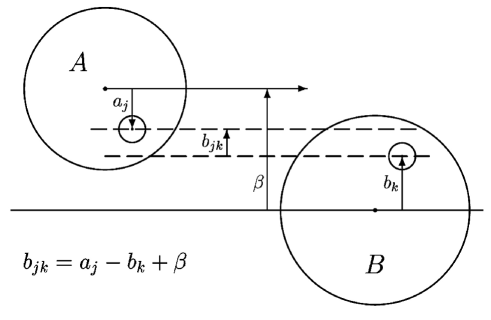
Appendix A Calculation of the variance of participants in one nucleus

The geometry of $AB$-collision is depicted in Fig.12. All $a_{j}$ and $b_{k}$ are the two-dimensional vectors in the impact parameter plane. In the framework of the classical (probabilistic) approach [18] the dimensionless $\sigma(b)$ is the probability of inelastic interaction of two nucleons at the impact parameter value $b$ (see also (13)). The $T_{A}$ and $T_{B}$ are the profile functions of the colliding nuclei $A$ and $B$. We are implying that for heavy nuclei the factorization takes place:

$$T_{A}(a_{1},...,a_{A})=\prod_{j=1}^{A}T_{A}(a_{j})\ .$$ (31)

Convenient to introduce the abbreviated notation:

$$\int\hat{d}a=\int T_{A}(a)\,da=1\ .$$ (32)

All integrations imply the integration over two-dimensional vectors in the impact parameter plane. In new notation the (10) takes the form

$$\langle X\rangle\equiv\langle\langle\overline{X}\rangle_{B}\rangle_{A}=\int\overline{X}\prod_{{k}=1}^{B}\hat{d}b_{k}\prod_{{j}=1}^{A}\hat{d}a_{j}\ .$$ (33)

Recall that here $\overline{X}$ means average of some variate $X$ at fixed positions of all nucleons in $A$ and $B$; $\langle{\ }\rangle_{A}$ and $\langle{\ }\rangle_{B}$ mean averaging over positions of these nucleons.

Refer to caption

Figure 12: Geometry of $AB$-collision.

We introduce the set of variates $X_{1},...,X_{A}$ (each can be equal only to 0 or 1) by the following way: $X_{j}=1$, if $j$-th nucleon of the nucleus $A$ interacts with some nucleons of the nucleus $B$ and $X_{j}=0$, if $j$-th nucleon doesn’t interact with any nucleons of the nucleus $B$. The number of participants (wounded nucleons) in the nucleus $A$ in a given collision at the impact parameter $\beta$ is equal to the sum of these variates:

$$N^{A}_{w}(\beta)=\sum_{{j}=1}^{A}X_{j}\ .$$ (34)

Then we have for the mean value:

$$\langle N^{A}_{w}(\beta)\rangle=\sum_{{j}=1}^{A}\langle X_{j}\rangle=\sum_{{j}=1}^{A}\langle\langle\overline{X_{j}}\rangle_{B}\rangle_{A}$$ (35)

and for the variance of $N^{A}_{w}(\beta)$:

$$V[N^{A}_{w}(\beta)]\equiv\langle{N_{w}^{A}(\beta)}^{2}\rangle-\langle N^{A}_{w}(\beta)\rangle^{2}\ ,\hskip 28.45274pt\langle{N_{w}^{A}(\beta)}^{2}\rangle=\langle(\sum_{{j}=1}^{A}X_{j})^{2}\rangle\ .$$ (36)

At first we calculate the mean value (35). We denote by $q_{j}$ and $p_{j}$ the probabilities that the variate $X_{j}$ will be equal to 0 or 1 correspondingly. Clear that for given configurations of nucleons $\{a_{j}\}$ and $\{b_{k}\}$ in nuclei $A$ and $B$:

$$q_{j}=\prod_{{k}=1}^{B}(1-\sigma_{jk})\ ,\hskip 28.45274ptp_{j}=1-q_{j}\ ,$$ (37)

where

$$\sigma_{jk}\equiv\sigma(a_{j}-b_{k}+\beta)$$ (38)

and

$$\overline{X_{j}}=0\cdot q_{j}+1\cdot p_{j}=p_{j}\ .$$ (39)

Note that $p_{j}$ and $q_{j}$ are the functions of $a_{j}$, $b_{1}$,…,$b_{B}$ and $\beta$:

$$q_{j}=q_{j}(a_{j},\{b_{k}\},\beta)\ ,\hskip 28.45274ptp_{j}=p_{j}(a_{j},\{b_{k}\},\beta)\ .$$ (40)

Recall that we restrict our consideration by the region of the impact parameter $\beta<R_{A}+R_{B}$ where the probability of inelastic nucleus-nucleus interaction $\sigma_{\!AB}(\beta)$ is close to unity. Otherwise one has to introduce in formula (37) for $q_{j}$ the factor $1/\sigma_{\!AB}(\beta)$, where

$$\sigma_{\!AB}(\beta)=1-\langle\langle{\prod_{{j}=1}^{A}\prod_{{k}=1}^{B}(1-\sigma_{jk})}\rangle_{A}\rangle_{B}$$ (41)

and $\sigma_{\!AB}=\int d\beta\,\sigma_{\!AB}(\beta)$ is so-called production cross section, which can’t be calculated in a closed form.

Substituting (37)-(39) into (35) we have

$$\langle N^{A}_{w}(\beta)\rangle=A-\sum_{{j}=1}^{A}\langle\langle{q_{j}}\rangle_{B}\rangle_{A}\ .$$ (42)

Averaging at first on positions of the nucleons in the nucleus $B$, we find

$$\langle q_{j}\rangle_{B}=(1-\sigma_{j})^{B}\ ,$$

where we have introduced the short notation:

$$\sigma_{j}\equiv\int\hat{d}b_{1}\sigma_{j1}=\int db_{1}T_{B}(b_{1})\sigma(a_{j}-b_{1}+\beta)\ .$$ (43)

Averaging now on positions of the nucleons in the nucleus $A$, we have

$$\langle\langle{q_{j}}\rangle_{B}\rangle_{A}=\int\hat{d}a_{j}(1-\sigma_{j})^{B}\ ,$$ (44)

which is the same for any $j$, as the $a_{j}$ is the integration variable:

$$\langle\langle{q_{j}}\rangle_{B}\rangle_{A}=\int da_{1}T_{A}(a_{1})(1-\sigma_{1})^{B}\equiv Q(\beta)\ .$$ (45)

Then by (42) we find

$$\langle N^{A}_{w}(\beta)\rangle=A(1-Q(\beta))=AP(\beta)\ ,$$ (46)

which coincides with formula (1) of the text, if one takes into account the connection

$$\sigma_{j}=f_{B}(a_{j}+\beta)$$ (47)

(see (5) and (43)). We see that the result for the mean number of participants (46) is the same as in the optical approximation (8).

We calculate now by the same way the variance of $N^{A}_{w}(\beta)$. By (36) we have:

$$\langle{N_{w}^{A}(\beta)}^{2}\rangle=\sum_{{j_{1}\neq j_{2}}=1}^{A}\langle X_{j_{1}}X_{j_{2}}\rangle+\sum_{{j}=1}^{A}\langle X^{2}_{j}\rangle\ .$$ (48)

Note that the $\langle X_{j_{1}}X_{j_{2}}\rangle$ can’t be reduced to the product $\langle X_{j_{1}}\rangle\langle X_{j_{2}}\rangle$. Just in this point the optical approximation breaks for AB collisions.

Since by (39)

$$\overline{X^{2}_{j}}=\overline{X_{j}}=p_{j}\ ,$$

then for the first sum in (48) we find:

$$\sum_{{j}=1}^{A}\langle X^{2}_{j}\rangle=\sum_{{j}=1}^{A}\langle X_{j}\rangle=\langle{N_{w}^{A}(\beta)}\rangle=AP(\beta)\ .$$ (49)

Because

$$\overline{X_{j_{1}}X_{j_{2}}}=\overline{X_{j_{1}}}\cdot\overline{X_{j_{2}}}=p_{j_{1}}p_{j_{2}}=1-q_{j_{1}}-q_{j_{2}}+q_{j_{1}}q_{j_{2}}\ ,$$

for the second sum in (48) using (45) we have:

$$\sum_{{j_{1}\neq j_{2}}=1}^{A}\langle X_{j_{1}}X_{j_{2}}\rangle=A(A-1)[1-2Q(\beta)+Q^{(12)}(\beta)]\ ,$$ (50)

where we have introduced

$$Q^{(12)}(\beta)\equiv\frac{1}{A(A-1)}\sum_{{j_{1}\neq j_{2}}=1}^{A}\langle\langle{q_{j_{1}}q_{j_{2}}}\rangle_{B}\rangle_{A}\ .$$ (51)

We calculate now $Q^{(12)}(\beta)$. Averaging again at first on positions of the nucleons in the nucleus $B$, we have

$$\langle q_{j_{1}}q_{j_{2}}\rangle_{B}=(1-\sigma_{j_{1}}-\sigma_{j_{2}}+\sigma^{(j_{1}j_{2})})^{B}\ ,$$

where $\sigma_{j_{1}}$ and $\sigma_{j_{2}}$ are given by (43) and

$$\sigma^{(j_{1}j_{2})}\equiv\int\hat{d}b_{1}\sigma_{j_{1}1}\sigma_{j_{2}1}=\int db_{1}T_{B}(b_{1})\sigma(a_{j_{1}}-b_{1}+\beta)\sigma(a_{j_{2}}-b_{1}+\beta)\ .$$ (52)

Then averaging on positions of the nucleons in the nucleus $A$ one can rewright (51) as follows

$$Q^{(12)}(\beta)=\int da_{1}da_{2}T_{A}(a_{1})T_{A}(a_{2})(1-\sigma_{1}-\sigma_{2}+\sigma^{(12)})^{B}\ ,$$ (53)

where by (52)

$$\sigma^{(12)}=\int\hat{d}b_{1}\sigma_{11}\sigma_{21}=\int db_{1}T_{B}(b_{1})\sigma(a_{1}\!-\!b_{1}\!+\!\beta)\sigma(a_{2}\!-\!b_{1}\!+\!\beta)\equiv g_{B}(a_{1}\!+\!\beta,a_{2}\!+\!\beta)$$ (54)

(see notation (6) of the text). Substituting (48), (49) and (50) into (36) we find for the variance of $N^{A}_{w}(\beta)$:

$$V[N^{A}_{w}(\beta)]=AQ(\beta)[1-Q(\beta)]+A(A\!-\!1)[Q^{(12)}(\beta)-Q^{2}(\beta)]\ ,$$

which coincides with the formula (2) of the text if we take into account (47), (53) and (54).

Appendix B Correlation between the numbers of participants in colliding nuclei at fixed centrality

The calculations are similar to ones in appendix A (we use the same notations). Along with the set of variates $X_{1},...,X_{A}$ we introduce in the symmetric way the set of variates $\widetilde{X}_{1},...,\widetilde{X}_{B}$ (each can be again equal only to 0 or 1). $\widetilde{X}_{k}=0(1)$ if $k$-th nucleon of the nucleus $B$ doesn’t interact (interacts) with nucleons of the nucleus $A$. Then similarly to (34) for the number of participants (wounded nucleons) in a given event in the nucleus $B$ we have:

$$N^{B}_{w}(\beta)=\sum_{{k}=1}^{B}\widetilde{X}_{k}\ .$$ (55)

Then

$$\langle N_{w}^{A}(\beta)N^{B}_{w}(\beta)\rangle=\sum_{{j}=1}^{A}\sum_{{k}=1}^{B}\langle\langle\overline{X_{j}\widetilde{X}_{k}}\rangle_{B}\rangle_{A}$$ (56)

and similarly to (39)

$$\overline{X_{j}\widetilde{X}_{k}}=P_{jk}(1,1)\ ,$$ (57)

where the $P_{jk}(1,1)$ is the probability that the both variates $X_{j}$ and $\widetilde{X}_{k}$ will be equal to 1. For the probability $P_{jk}(1,1)$ one finds

$$P_{jk}(1,1)=\sigma_{jk}+(1-\sigma_{jk})\rho_{jk}\widetilde{\rho}_{jk}\ ,$$ (58)

where $\sigma_{jk}$ is the probability of the interaction of the $j$-th nucleon of the nucleus $A$ with the $k$-th nucleon of the nucleus $B$ (see formula (38)) and $\rho_{jk}$ is the probability of the interaction of the $j$-th nucleon of the nucleus $A$ with at least one nucleon of the nucleus $B$ except the $k$-th nucleon (correspondingly $\widetilde{\rho}_{jk}$ is the probability of the interaction of the $k$-th nucleon of the nucleus $B$ with at least one nucleon of the nucleus $A$ except the $j$-th nucleon):

$$\rho_{jk}=1-\!\!\!\!\!\!\prod^{B}_{k^{\prime}=1(k^{\prime}\neq k)}\!\!\!(1-\sigma_{jk^{\prime}})\ ,\hskip 56.9055pt\widetilde{\rho}_{jk}=1-\!\!\!\!\!\!\prod^{A}_{j^{\prime}=1(j^{\prime}\neq j)}\!\!\!(1-\sigma_{j^{\prime}k})\ .$$ (59)

Combining (56)–(59) and acting as in appendix A we find the formulae (19)–(22) of the text.

Appendix C Fluctuations of the number of collisions

In this appendix we calculate the variance of the number of NN-collisions in AB-interaction at fixed value of centrality in the framework of the approach under consideration.

To calculate the number of collisions we define the set of the variates $Y_{1},...,Y_{A}$, which can take on a value from 0 to $B$. If in the given event the $j$-th nucleon of the nucleus $A$ interacts with $n$ nucleons of the nucleus $B$, then $Y_{j}=n$. The number of NN-collisions in the given event at the impact parameter $\beta$ can be expressed through these variates as follows:

$$N_{coll}(\beta)=\sum_{{j}=1}^{A}Y_{j}$$ (60)

Clear that again (see appendix A):

$$P(Y_{j}=0)=q_{j}=\prod_{{k}=1}^{B}(1-\sigma_{jk})$$ (61)

To calculate $P(Y_{j}=n)$ for $n=1,...,B$ we introduce $\{k_{1},...,k_{n}\}$ - the sampling from the set $\{1,...,B\}$ and $\{k_{n+1},...,k_{B}\}$ - the rest after sampling. Then

$$P(Y_{j}=n)=\sum_{\{k_{1},...,k_{n}\}}\sigma_{jk_{1}}...\sigma_{jk_{n}}(1-\sigma_{jk_{n+1}})...(1-\sigma_{jk_{B}})$$ (62)

First we again calculate the mean value of the number of collisions:

$$\langle N_{coll}(\beta)\rangle=\sum_{{j}=1}^{A}\langle\langle\overline{Y_{j}}\rangle_{B}\rangle_{A}\ .$$ (63)

For a given configuration $\{a_{j}\}$ and $\{b_{k}\}$ we have:

$$\overline{Y_{j}}=\sum_{n=0}^{B}\,n\,P(Y_{j}=n)\ .$$ (64)

Using (62) and averaging on positions of the nucleons in the nucleus $B$, one finds

$$\langle\overline{Y_{j}}\rangle_{B}=\sum_{n=0}^{B}\,n\,C_{B}^{n}\sigma_{j}^{n}(1-\sigma_{j})^{B-n}=B\,\sigma_{j}\ .$$ (65)

We use the same notations as in appendix A (see (43)). Averaging then on positions of the nucleons in the nucleus $A$, we finally find:

$$\langle N_{coll}(\beta)\rangle=AB\chi(\beta)\ ,$$ (66)

where

$$\chi(\beta)\equiv\int\hat{d}a_{1}\sigma_{1}=\int\hat{d}a_{1}\hat{d}b_{1}\sigma_{11}=\int da_{1}db_{1}T_{A}(a_{1})T_{B}(b_{1})\sigma(a_{1}-b_{1}+\beta)\ ,$$ (67)

and at $r_{N}\ll R_{A},R_{B}$

$$\chi(\beta)\approx\sigma_{\!N\!N}\int da_{1}T_{A}(a_{1})T_{B}(a_{1}+\beta)\ ,$$ (68)

which coincides with the formulae (23) and (24) of the text. Comparing (66) and (29) we see that the result for the mean number of collisions is the same as in the optical approximation.

In the rest of the appendix we calculate the variance of the number of collisions. To calculate the variance:

$$V[N_{coll}(\beta)]\equiv\langle{N^{2}_{coll}(\beta)}\rangle-\langle N_{coll}(\beta)\rangle^{2}$$ (69)

one has to calculate

$$\langle{N^{2}_{coll}(\beta)}\rangle=\langle(\sum_{{j}=1}^{A}Y_{j})^{2}\rangle=\sum_{{j_{1}\neq j_{2}}=1}^{A}\langle Y_{j_{1}}Y_{j_{2}}\rangle+\sum_{{j}=1}^{A}\langle Y^{2}_{j}\rangle\ .$$ (70)

So we have to calculate the following two sums:

$$\sum_{{j_{1}\neq j_{2}}=1}^{A}\langle Y_{j_{1}}Y_{j_{2}}\rangle=\sum_{{j_{1}\neq j_{2}}=1}^{A}\langle\langle\overline{Y_{j_{1}}Y_{j_{2}}}\rangle_{B}\rangle_{A}$$ (71)

and

$$\sum_{{j}=1}^{A}\langle Y^{2}_{j}\rangle=\sum_{{j}=1}^{A}\langle\langle\overline{Y^{2}_{j}}\rangle_{B}\rangle_{A}\ .$$ (72)

To calculate the first sum we denote by $k^{\prime}_{1},...,k^{\prime}_{n}$ - the indices of the nucleons of the nucleus $B$, which interact only with the nucleon $j_{1}$ of the nucleus $A$. By $k^{\prime\prime}_{1},...,k^{\prime\prime}_{m}$ we denote the indices of the nucleons, which interact only with the nucleon $j_{2}$ of the nucleus $A$ and by $\overline{k}_{1},...,\overline{k}_{r}$ we denote the indices of the nucleons, which interact with both nucleons $j_{1}$ and $j_{2}$. By $k_{1},...,k_{B-n-m-r}$ we denote the indices of the nucleons of the nucleus $B$, which don’t interact with the nucleons $j_{1}$ and $j_{2}$ of the nucleus $A$. Then the probability $p_{j_{1}j_{2}}$ of such event in these notations is equal to

$$p_{j_{1}j_{2}}=p_{j_{1}}p_{j_{2}}\ ,$$ (73)

where

$$p_{j_{1}}=\prod_{i=1}^{r}\sigma_{j_{1}\overline{k}_{i}}\prod_{i=1}^{n}\sigma_{j_{1}k^{\prime}_{i}}\prod_{i=1}^{m}(1-\sigma_{j_{1}k^{\prime\prime}_{i}})\prod_{i=1}^{B-r-m-n}(1-\sigma_{j_{1}k_{i}})\ ,$$ (74)
$$p_{j_{2}}=\prod_{i=1}^{r}\sigma_{j_{2}\overline{k}_{i}}\prod_{i=1}^{n}(1-\sigma_{j_{2}k^{\prime}_{i}})\prod_{i=1}^{m}\sigma_{j_{2}k^{\prime\prime}_{i}}\prod_{i=1}^{B-r-m-n}(1-\sigma_{j_{2}k_{i}})\ .$$ (75)

Using (74) and (75) we can rewrite $p_{j_{1}j_{2}}$ in the following form

$$p_{j_{1}j_{2}}=\prod_{i=1}^{r}\sigma_{j_{1}\overline{k}_{i}}\sigma_{j_{2}\overline{k}_{i}}\prod_{i=1}^{n}\sigma_{j_{1}k^{\prime}_{i}}(1-\sigma_{j_{2}k^{\prime}_{i}})\prod_{i=1}^{m}(1-\sigma_{j_{1}k^{\prime\prime}_{i}})\sigma_{j_{2}k^{\prime\prime}_{i}}\!\!\prod_{i=1}^{B-r-m-n}\!\!(1-\sigma_{j_{1}k_{i}}-\sigma_{j_{2}k_{i}}+\sigma_{j_{1}k_{i}}\sigma_{j_{2}k_{i}})\ .$$ (76)

The probability $P_{j_{1}j_{2}}(n,m,r)$ that the nucleons $j_{1}$ and $j_{2}$ of the nucleus $A$ interact separately with $n$ and $m$ nucleons of the nucleus $B$ and at that else simultaneously with $r$ nucleons of the nucleus $B$ is equal to

$$P_{j_{1}j_{2}}(n,m,r)=\sum p_{j_{1}j_{2}}\ ,$$ (77)

where the sum means summing on all possible three sampling $\{k^{\prime}_{1},...,k^{\prime}_{n}\}$, $\{k^{\prime\prime}_{1},...,k^{\prime\prime}_{m}\}$, $\{\overline{k}_{1},...,\overline{k}_{r}\}$ from the set $\{1,...,B\}$. After averaging (77) on positions of the nucleons in the nucleus $B$ we find

$$\langle P_{j_{1}j_{2}}(n,m,r)\rangle_{B}=\frac{B!}{n!m!r!(B-r-m-n)!}z^{r}(y-z)^{m}(x-z)^{n}(1-x-y+z)^{B-r-m-n}\ ,$$ (78)

where we have used the short notations:

$$x=\sigma_{j_{1}}\ ,\hskip 28.45274pty=\sigma_{j_{2}}\ ,\hskip 28.45274ptz=\sigma^{(j_{1}j_{2})}\ .\hskip 28.45274pt$$ (79)

The $\sigma_{j_{1}}$ and $\sigma_{j_{2}}$ are defined by (43) and the $\sigma^{(j_{1}j_{2})}$ is defined by (52) in appendix A. Then for the components of the first sum (71) we have

$$\langle{\overline{Y_{j_{1}}Y_{j_{2}}}}\rangle_{B}=\sum_{r=0}^{B}\sum_{m=0}^{B-r}\sum_{n=0}^{B-r-m}(m\!+\!r)(n\!+\!r)\langle P_{j_{1}j_{2}}(n,m,r)\rangle_{B}\ .$$ (80)

After substitution of (78) in (80) the lengthy but straightforward calculation leads to the simple answer

$$\langle{\overline{Y_{j_{1}}Y_{j_{2}}}}\rangle_{B}=Bz+B(B\!-\!1)xy=B\sigma^{(j_{1}j_{2})}+B(B\!-\!1)\sigma_{j_{1}}\sigma_{j_{2}}\ .$$ (81)

For the components of the second sum (72) the similar but much more simple calculation gives

$$\langle{\overline{Y_{j}^{2}}}\rangle_{B}=B\sigma_{j}+B(B\!-1\!)\sigma_{j}^{2}\ .$$ (82)

Averaging now on positions of the nucleons in the nucleus $A$, we can rewrite (70) as

$$\langle{N^{2}_{coll}(\beta)}\rangle=B\left[\sum_{{j_{1}\neq j_{2}}=1}^{A}\left(\langle{\sigma^{(j_{1}j_{2})}}\rangle_{A}+(B\!-\!1)\langle{\sigma_{j_{1}}\sigma_{j_{2}}}\rangle_{A}\right)+\sum_{{j}=1}^{A}\left(\langle{\sigma_{j}}\rangle_{A}+(B\!-\!1)\langle{\sigma_{j}^{2}}\rangle_{A}\right)\right]=$$
$$=B\left[A(A\!-\!1)\int\hat{d}a_{1}\hat{d}a_{2}\left(\langle{\sigma^{(12)}}\rangle_{A}+(B\!-\!1)\langle{\sigma_{1}\sigma_{2}}\rangle_{A}\right)+A\int\hat{d}a_{1}\left(\langle{\sigma_{1}}\rangle_{A}+(B\!-\!1)\langle{\sigma_{1}^{2}}\rangle_{A}\right)\right]$$

Recalling now that $\sigma_{1}$, $\sigma_{2}$ and $\sigma^{(12)}$ are given by the formulae (43) and (54) of the appendix A, we obtain

$$\langle{N^{2}_{coll}(\beta)}\rangle=AB[\chi(\beta)+(B\!-\!1)\chi_{1}(\beta)+(A\!-\!1)\widetilde{\chi}_{1}(\beta)+(A\!-\!1)(B\!-\!1)\chi^{2}(\beta)]$$ (83)

with $\chi(\beta)$, $\chi_{1}(\beta)$ and $\widetilde{\chi}_{1}(\beta)$ defined by the formulae (24), (26) and (27) of the text. Using now the definition (69) and taking into account the formula (66) for $\langle N_{coll}(\beta)\rangle$ we come to the expression (25) of the text for the variance of the number of collisions.

References

  • [1] C. Alt et al. (NA49 Collaboration), Phys. Rev. C 75, 064904 (2007).
  • [2] C. Alt et al., Phys. Rev. C 78, 034914 (2008).
  • [3] T. Anticic et al. (NA49 Collaboration), Phys. Rev. C 79, 044904 (2009).
  • [4] A. Adare et al. (PHENIX Collaboration), Phys. Rev. C 78, 044902 (2008).
  • [5] W. Broniowski, P. Bozek, M. Rybczynski, Phys. Rev. C 76, 054905 (2007).
  • [6] M. Gazdzicki, M. Gorenstein, Phys. Lett. B 640, 155 (2006).
  • [7] V. P. Konchakovski et al., Phys. Rev. C 73, 034902 (2006).
  • [8] M. Stephanov, K. Rajagopal, E. Shuryak, Phys. Rev. D 60, 114028 (1999).
  • [9] M. Gazdzicki for the NA61/SHINE Collaboration, PoS C POD2006, 016 (2006).
  • [10] M. A. Braun, C. Pajares, V. V. Vechernin, Phys. Lett. B493, 54 (2000).
  • [11] M. A. Braun, R. S. Kolevatov, C. Pajares, V. V. Vechernin, Eur. Phys. J. C 32, 535 (2004).
  • [12] V. V. Vechernin, R. S. Kolevatov, Phys. of Atom. Nucl. 70, 1797; 1809 (2007).
  • [13] N. Armesto, M. A. Braun, C. Pajares, Phys. Rev. C 75, 054902 (2007).
  • [14] N. Armesto, L. McLerran, C. Pajares, Nucl. Phys. A781, 201 (2007).
  • [15] L. Cunqueiro, E. G. Ferreiro, F. del Moral, C. Pajares, Phys. Rev. C 72, 024907 (2005).
  • [16] P. Brogueira, J. Dias de Deus, J. G. Milhano, Phys. Rev. C 76, 064901 (2007).
  • [17] D. Adamova et al. (CERES Collaboration), Nuclear Physics A 811, 179 (2008).
  • [18] A. Bialas, M. Bleszynski, W. Czyz, Nucl. Phys. B111, 461 (1976).
  • [19] W. Czyz, L. C. Maximon, Annals of Physics 52, 59 (1969).
  • [20] J. Formanek, Nucl. Phys. B12, 441 (1969).
  • [21] Cheuk-Yin Wong, Introduction to high-energy heavy-ion collisions. World Scientific, Singapore, 1994, 519pp.
  • [22] R. Vogt, Ultrarelativistic heavy-ion collisions. Elsevier B. V., Amsterdam, 2007, 488pp.
  • [23] K. G. Boreskov, A. B. Kaidalov, Yad. Fiz. 48, 575 (1988).
  • [24] A. S. Pak, A. V. Tarasov, V. V. Uzhinskij, C. Tseren, Yad. Fiz. 30, 102 (1979).
  • [25] M. A. Braun, Yad. Fiz. 45, 1625 (1987); 48, 409 (1988); 51, 1722 (1990).
  • [26] L. L. Frankfurt, M. I. Strikman, Phys. Rep. 76, 215, (1981); 160, 235 (1988).