Invisible, but important

COrE
Cosmic Origins Explorer
A White Paper

Mission and programmatics working group
F. R. Bouchet, P. de Bernardis, B. Maffei, P. Natoli, M. Piat, N. Ponthieu, R. Stompor

Instrument working group
B. Maffei, M. Bersanelli, P. Bielewicz, P. Camus, P. de Bernardis, M. De Petris, P. Mauskopf, S. Masi, F. Nati, T. Peacocke, F. Piacentini, L. Piccirillo, M. Piat, G. Pisano, M. Salatino, R. Stompor, S. Withington,

Science working group
M. Bucher, M. Avilles, D. Barbosa, N. Bartolo, R. Battye, J.-P. Bernard, F. Boulanger, A. Challinor, S. Chongchitnan, S. Colafrancesco, T. Ensslin, J. Fergusson, P. Ferreira, K. Ferriere, F. Finelli, J. García-Bellido, S. Galli, C. Gauthier, M. Haverkorn, M. Hindmarsh, A. Jaffe, M. Kunz, J. Lesgourgues, A. Liddle, M. Liguori, P. Marchegiani, S. Matarrese, A. Melchiorri, P. Mukherjee, L. Pagano, D. Paoletti, H. Peiris, L. Perroto, C. Rath, J. Rubiño Martin, C. Rath, P. Shellard, J. Urrestilla, B. Van Tent, L. Verde, B. Wandelt

Foregrounds working group
C. Burigana, J. Delabrouille, C. Armitage-Caplan, A. Banday, S. Basak, A. Bonaldi, D. Clements, G. De Zotti, C. Dickinson, J. Dunkley, M. Lopez-Caniego, E. Martínez-Gonzalez, M. Negrello, S. Ricciardi, L. Toffolatti

This White Paper is an extended version of a proposal document that was submitted to ESA in December 2010 in response to a Call for Proposals within the framework of ESA’s Cosmic Vision 2015-25. The proposal is the product of the cosmic microwave background observation communities from France, Italy, Spain, and the United Kingdom, as well as several other European countries (presently Denmark, Germany, Ireland, the Netherlands, Norway, Portugal, Sweden, Switzerland). The US community as represented by the PPPT group and its chairman (S. Hanany) has expressed strong interest in an extensive collaboration if this proposal is successful. A full list of the people currently involved with COrE may be found at our website: http://www.core-mission.org. Above we have listed those members of the COrE community who have contributed most actively in preparing the proposal and white paper under the working group to which they have contributed the most.

Revised version: 28 April 2011

BOO

ABSTRACT

COrE (Cosmic Origins Explorer) is a fourth-generation full-sky, microwave-band satellite recently proposed to ESA within Cosmic Vision 2015-2025. COrE will map the polarization of the microwave sky with such a high precision that tensor modes produced by the inflationary expansion are detected at more than 3$\sigma$ even if they are 0.1% of the scalar modes. This is a factor about 50 times better than what PLANCK can achieve. COrE will provide maps of the microwave sky in 15 frequency bands, ranging from 45 GHz to 795 GHz, with an angular resolution ranging from 23 arcmin (45 GHz) to 1.3 arcmin (795 GHz) and sensitivities roughly 10–30 times better than PLANCK (depending on the frequency channel). The COrE mission will lead to breakthrough science in a wide range of areas, from primordial cosmology to galactic and extragalactic science. COrE is designed to detect the primordial gravitational waves generated during the epoch of cosmic inflation at more than $3\sigma$ for $r=(T/S)\geq 10^{-3}$. It will also measure the CMB gravitational lensing deflection power spectrum to the cosmic variance limit on all linear scales, allowing us to probe absolute neutrino masses better than laboratory experiments and down to plausible values suggested by the neutrino oscillation data. COrE will also search for primordial non-Gaussianity with significant improvements over PLANCK in its ability to constrain the shape and amplitude of non-Gaussianity. In the areas of galactic and extragalactic science, in its highest frequency channels COrE will provide maps of the galactic polarized dust emission allowing us to map the galactic magnetic field in areas of diffuse emission not otherwise accessible to probe the initial conditions for star formation. COrE will also map the galactic synchrotron emission thirty times better than PLANCK. This White Paper reviews the COrE science program, our simulations on foreground subtraction, and the proposed instrumental configuration.

1 Overview of polarized microwave sky

COrE is a fourth-generation full-sky, microwave-band satellite that has been proposed to ESA within the context of Cosmic Vision 2015-2025 to follow on the successes of the COBE, WMAP, and PLANCK space missions. COrE will map the polarization of the microwave sky with a relative precision comparable to that of the temperature maps that PLANCK is now in the process of delivering. COrE will provide maps of the microwave sky in 15 frequency bands, ranging from 45 GHz to 795 GHz with an angular resolution roughly comparable to PLANCK and a sensitivity 10–30 times better (depending on the frequency channel). The sensitivity of COrE, which nominally corresponds to over 250 years of PLANCK integration time, matches the need to observe the polarized signal whose level is only a few percent of the temperature anisotropy.

The COrE mission will lead to breakthrough science in a wide variety of areas, ranging from primordial cosmology to galactic and extragalactic science. COrE is designed to detect the primordial gravitational waves generated during the epoch of cosmic inflation at more than $3\sigma$ for $r=(T/S)\geq 10^{-3}$. COrE will also measure the CMB gravitational lensing power spectrum with unprecedented precision, allowing us to probe absolute neutrino masses better than is possible in laboratory experiments and down to plausible values suggested by the neutrino oscillation data. COrE will search for primordial non-Gaussianity, essentially at the theoretical limit of what is possible with the CMB. While PLANCK will measure the E-mode polarization with a signal-to-noise oscillating in the neighborhood of unity for $\ell\mathrel{\raise 1.29167pt\hbox{$<$}\mkern-14.0mu\lower 2.58334pt\hbox{$\sim$}}800,$ COrE will provide $(S/N)\gg 1$ maps up to $\ell\approx 2000$—a major step forward since it is the number of independent resolution elements that determines the lensing science and non-Gaussianity search capabilities of a survey. On the front of galactic and extragalactic science, in its highest frequency channels COrE will provide maps of the galactic polarized dust emission with a precision not possible from the ground. This data will allow us to map the galactic magnetic field in areas of diffuse emission not otherwise accessible, thus probing the initial conditions for star formation. COrE will also map the galactic synchrotron emission ten times better than PLANCK and WMAP at 45 GHz where the Faraday rotation is small. In the highest frequency channels CORE’s angular resolution will be diffraction limited with a beam size of $1.3^{\prime}$ full width at half maximum (fwhm). This enhanced resolution combined with COrE’s exquisite sensitivity will lead to the discovery of numerous compact sources across the whole sky with well-defined selection criteria.

We review the diverse science objectives motivating the mission, formulate the instrumental requirements for achieving these objectives, and discuss the procedure for separating all the many components contributing to the observed microwave sky in this frequency range. An adequate and reliable component separation is a prerequisite for achieving the targeted science objectives. Finally we describe the proposed instrument and the proposed technology.

Observations of the microwave and far infrared sky have revolutionized our understanding of the origins of the Universe and the processes at play within our galaxy and beyond. Before proceeding to a detailed analysis of some of the highlights of the new science that will be made possible with COrE, it is appropriate to review what is known, mainly from temperature maps but also from the presently available polarization data, concerning the several components emitting in the microwave bands and then quickly review the physical mechanisms causing this emission to be partially polarized, with a view toward understanding qualitatively the new science that can be extracted.

We begin our tour in the center of COrE’s broad frequency coverage. For the temperature and polarization anisotropies, the central channels from about 70–220 GHz offer a relatively clean window through which the primordial CMB anisotropies dominate. At lower frequencies, a non-thermal galactic synchrotron component becomes an increasingly dominant contribution to the anisotropic signal. The synchrotron component arises from the interaction of cosmic rays with the galactic magnetic field and provides invaluable information to constrain the galactic magnetic field. This component has a spectral index redder than a blackbody by approximately three inverse powers in frequency, allowing it to be removed through this differing frequency dependence. The WMAP data has provided a wealth of information concerning the degree of polarization of this synchrotron emission, providing one of the inputs for the COrE polarization cleaning forecasts. Nevertheless a more precise template will be needed, hence the presence of 45 GHz channel. At low frequencies, there is also a free-free component, arising from bremsstrahlung of the hot HII regions, tightly correlated with H$\alpha$ emission, which serves as a useful tracer. This emission however is not intrinsically polarized. At the low end of the spectrum, mostly below the frequency coverage of COrE, one also has evidence for spinning dust emission. The details and degree of polarization of this emission are not presently well understood.

Figure 1: Inflationary prediction for the CMB temperature and polarization anisotropies for the scalar and tensor modes. The horizontal axis indicates the multipole number $\ell$ and the vertical axis indicates $\ell(\ell+1)C_{\ell}^{AB}/(2\pi)$ in units of $(\mu K)^{2}$, which is roughly equivalent to the derivative of the power spectrum with respect to $\ln\ell$. The green curves indicate the TT, TE, and EE power spectra (from top to bottom) generated by the scalar mode assuming the parameters from the best-fit model from WMAP seven-year data ($H_{0}=71.4\,{\rm km~{}s^{-1}~{}Mpc^{-1}}$, $\Omega_{b}=0.045$, $\Omega_{cdm}=0.220$, $\Omega_{\Lambda}=0.73$, $\tau=0.086$, and $n_{s}=0.969$). The BB scalar component (indicated by the heavy red curve) results from the gravitational lensing of the EE polarized CMB anisotropy at the last scattering surface $z\approx 1100$ by structures situated mainly around redshift $z\approx 2$. The top three blue curves (from top to bottom on the left) indicate the TT, TE, BB, and EE spectra resulting from the tensor mode assuming a scale-invariant ($n_{T}=0$) primordial spectrum and a tensor-to-scalar ratio $(T/S)$ of $0.1$, and the solid black curves indicate the BB spectra for the descending values of $(T/S)=r=0.1,0.01,0.001$ and $0.0001.$ For the TE cross-correlations we have plotted the log of the absolute value, hence the downward spikes which correspond to sign changes.

Above the so-called CMB channels, above around 250 GHz, a component of cold ($T\approx 20K$) dust starts to become the dominant contribution to the anisotropies as one pushes into the exponentially falling Wien regime of the CMB blackbody spectrum. The physics of the dust grains of the interstellar medium is complex and only partially understood. Our understanding is summarized by empirical models of the grain populations drawing from a variety of observational inputs (frequency dependence of reddening including the presence of absorption features, polarization of starlight, infrared emission,…) as well as more physical arguments (bottom-up modelling informed by cosmic element abundances). The infrared emission can be described approximately with a blackbody at the dust temperature and an emissivity index in the neighborhood of $\alpha=1.7.$ Presently the most widely used dust model has two dust components with separate temperatures and emissivity indices.

$\nu$	$\theta_{fwhm}$	$n_{det}$	Temp (I)		Pol (Q,U)
			$\mu K\cdot$arcmin		$\mu K\cdot$arcmin
GHz	arcmin		RJ	CMB	RJ	CMB
23	52.8	2	413	418	584	592
33	39.6	2	413	424	584	600
41	30.6	4	365	381	516	539
61	21.0	4	438	481	619	681
94	13.2	8	413	516	584	729

WMAP (9 year mission)

$\nu$ $n_{unpol}$ $n_{pol}$ $\theta_{fwhm}$ Temp (I) Pol (Q,U) $\mu K\cdot$arcmin $\mu K\cdot$arcmin GHz arcmin RJ CMB RJ CMB 30 4 4 32.7 198.5 203.2 280.7 287.4 44 6 6 27.9 228.0 239.6 322.4 338.9 70 12 12 13.0 186.5 211.2 263.7 298.7 100 8 8 9.9 23.9 31.3 33.9 44.2 143 11 8 7.2 11.9 20.1 19.7 33.3 217 12 8 4.9 9.4 28.5 16.3 49.4 353 12 8 4.7 7.6 107.0 13.2 185.3 545 3 0 4.7 6.8 $1.1\times 10^{3}$ — — 857 3 0 4.4 2.9 $8.3\times 10^{4}$ — —

PLANCK (30 month mission)

$\nu$	$(\Delta\nu)$	$n_{det}$	$\theta_{fwhm}$	Temp (I)		Pol (Q,U)
				$\mu K\cdot$arcmin		$\mu K\cdot$arcmin
$GHz$	$GHz$		arcmin	RJ	CMB	RJ	CMB
45	15	64	23.3	4.98	5.25	8.61	9.07
75	15	300	14.0	2.36	2.73	4.09	4.72
105	15	400	10.0	2.03	2.68	3.50	4.63
135	15	550	7.8	1.68	2.63	2.90	4.55
165	15	750	6.4	1.38	2.67	2.38	4.61
195	15	1150	5.4	1.07	2.63	1.84	4.54
225	15	1800	4.7	0.82	2.64	1.42	4.57
255	15	575	4.1	1.40	6.08	2.43	10.5
285	15	375	3.7	1.70	10.1	2.94	17.4
315	15	100	3.3	3.25	26.9	5.62	46.6
375	15	64	2.8	4.05	68.6	7.01	119
435	15	64	2.4	4.12	149	7.12	258
555	195	64	1.9	1.23	227	3.39	626
675	195	64	1.6	1.28	1320	3.52	3640
795	195	64	1.3	1.31	8070	3.60	22200

COrE summary (4 year mission)

Table 1: COrE performance summary compared to WMAP and PLANCK. The Planck numbers reported here are based on instrument performance as measured in flight and projected to the best current estimate of the mission lifetime (i.e., 30 months). In the low frequency channels the superior performance of COrE derives from a combination of the increased number of detectors and the more sensitive bolometer technology, which allows measurements to be made at nearly the quantum shot noise limit. For example at 45 GHz, the lowest frequency channel of COrE, the Planck-LFI integration time would have to be increased by approximately a factor of a thousand to match the COrE sensitivity. In the central channels this factor is reduced to about 100, because Planck-HFI, like COrE, already uses bolometers cooled to 0.1K. The COrE bolometers, however, are much more numerous than those of Planck and their individual perforance is closer to the quantum limit. For galactic and extragalactic science using polarization data, Planck is severely limited by the fact that the Planck-HFI channels at 545 GHz and 857 GHz lack polarization sensitive bolometers. Moreover, the angular resolution of COrE in the highest frequencies is diffraction limited whereas for PLANCK it is not. This is a major limitation because interstellar dust and many other sources of interest are best studied at these high frequencies. COrE will thus open a new window in mapping far infrared polarized emission. These high frequency channels require only a small fraction of the COrE resources, as they occupy a small portion of the focal plane area and contribute a small fraction to the total data rate transmitted to Earth. In Sec. 4.1 we propose a modification of the baseline, where the sensitivity at 795 GHz is increased by a factor of five, at negligible cost to the primordial science, but greatly enhancing the COrE capabilities for Galactic science.

Figure 2: CMB scalar and tensor anisotropies relative to PLANCK and COrE sensitivities We show again the scalar (blue and red) and tensor (black) anisotropies but now together with the PLANCK and CORE instrument noise in brown and magenta, respectively. The scalar anisotropies are the TT (top) and EE (bottom) spectra in blue and a BB lensing contribution (in red). These are relatively certain. The BB is shown for $r$ of $0.1,$ $0.01$ and $0.001$ in black (top to bottom). The solid brown and magenta curves show the instrument noise power spectra for PLANCK and COrE, and the dashed counterparts below indicate what sensitivity can be obtained by wide binning $(\Delta\ell)/\ell\approx 1.$ Modes of the CMB spectra lying above the solid noise curves are detected with $(S/N)\mathrel{\raise 1.29167pt\hbox{$>$}\mkern-14.0mu\lower 2.58334pt\hbox{$\sim$}}1,$ implying that measurements at higher instrumental sensitivity would result in marginal additional science value. On the other hand, CMB spectra lying between the solid and dashed sensitivity give a signal detectable when many modes are combined in the analysis. We see that for $\ell\mathrel{\raise 1.29167pt\hbox{$<$}\mkern-14.0mu\lower 2.58334pt\hbox{$\sim$}}800$ PLANCK the $C_{EE}$ measurements oscillate in and out of the $(S/N)=1$ threshold while for COrE modes up to $\ell\approx 2000$ are resolved with $(S/N)\gg 1.$ This means that for studies of non-Gaussianity one has about ten times as many resolution elements.

All these emission processes (with the exception of free-free) are partially polarized. The degree of polarization of the synchrotron emission is around 10% and that of the dust around 5–7% , although large uncertainties persist. For the primordial component, polarization can heuristically be understood as a measure of the CMB quadrupole moment as seen by a typical electron of last scattering, roughly proportional to the double derivative of the ‘temperature’ and the square of the mean distance between last and next-to-last scattering. This proportionality explains why the electric-type (E) polarization from the scalar perturbations receives an appreciable contribution from late-time reionization despite the fact that the reionization optical depth is quite small $(\tau\approx 0.087).$ This is the mechanism that allowed the WMAP polarization data to break the degeneracy between the amplitude of the primordial scalar perturbations $A$ and the reionization optical depth $\tau.$ Current observations of the polarization of the primordial CMB component are in good agreement with the scalar perturbations and cosmological parameters implicit from the temperature perturbations. Polarization provides a powerful cross check because it probes the other of the two quadratures of the cosmological perturbations.

The frontier of CMB polarization observations lies in searching for the B mode. The polarization field on the celestial sphere may be divided into two components: an E mode, which may be expressed by means of second derivatives acting on a potential, and a B mode where this pattern is rotated by $45^{\circ}.$ For scalar perturbations, which are the only ones that contribute to the matter power spectrum, only the E mode polarization is possible within linearized cosmological perturbation theory. Nonlinear corrections, which may be calculated reliably, contribute a gravitational lensing background (shown in red in Fig. 1) having a white noise spectrum at low multipole number $\ell.$ This ‘white noise’ at low $\ell$ has a magnitude of around $5\mu{\rm K}\cdot{\rm arcmin},$ the precise value depending slightly on the cosmological parameters. Any B mode with a black body spectrum beyond the level expected from lensing is the tell-tale sign of primordial gravitational waves from inflation, whose multipole spectral shape predictions are shown in Fig. 1 alongside the predictions for the scalar anisotropies, shown in green. The expected B-mode anisotropies from inflation is parameterized by the ratio of the primordial tensor perturbations relative to the scalar perturbations $(T/S)$ or $r.$

The current COrE concept does not attempt to ‘clean’ the gravitational lensing B mode, but rather accepts it as a background that can be well characterized and included in the analysis in the same way as one typically deals with instrument noise in CMB experiments. Hence the science requirement is to deliver a foreground cleaned map with an accuracy in the neighborhood of or slightly better than $5\mu K\cdot{\rm arcmin}$ after foreground subtraction. This requires a superior raw sensitivity in order to clean out the foregrounds.

The so-called “foregrounds” may, on the one hand, be considered a nuisance for primordial cosmology. They are the ‘dirt’ that must be removed to gain a glimpse at the pristine state of the primordial universe. But on the other hand, these foregrounds, which will be characterized with exquisite precision, constitute a gold mine for galactic and extragalactic science. In particular, the dust polarization maps produced, when combined with 21 cm maps to provide depth information, can be used to gain a better understanding of the galactic magnetic field, which according to equipartition arguments plays a key role in the dynamics of the interstellar medium. Numerous extragalactic polarized point sources will be discovered as well.

COrE will be competing with suborbital experiments likewise aiming to detect non-zero $(T/S)$ and carry out other components of the science program presented here. Suborbital experiments have indeed played and will continue to play an important role in developing and demonstrating new technology for space-based CMB observation. Nevertheless, suborbital experiments are substantially handicapped in a number of ways that are analyzed in detail in Sec. 4.4.

2 Science with COrE

2.1 Cosmic inflation

Inflation represents our current best understanding of the physics at play in the primordial Universe. Originally inflation was proposed to solve several cosmological conundrums—the famous horizon, flatness, smoothness, and monopole problems—using ideas from high-energy physics near the Planck scale, far beyond the reach of accelerator experiment. The successful resolution of these problems is a result of analyzing inflation using classical physics. However it was soon realized that when quantum effects are taken into account, inflation also provides a mechanism for explaining the nearly Gaussian nature of the primordial cosmological perturbations and explains the empirically deduced Harrison-Peebles-Zeldovich scale invariant spectrum of density perturbations. The scalar perturbations, which seed the large-scale structure seen today in the universe, has been extensively probed by WMAP, PLANCK, and other CMB experiments as well as galaxy surveys. Inflation however makes an additional prediction that has not yet been verified observationally—namely, that these scalar perturbations should be accompanied by primordial gravitational waves having a very red, scale-invariant spectrum. The confirmation of this prediction would provide a remarkable qualitatively new test of inflation. It would also establish the energy scale of inflation, providing invaluable data for physics near the Planck scale. The amplitude of these gravitational waves is parameterized by $r,$ the tensor-to-scalar ratio. PLANCK will be able to detect around $r\geq 0.1.$ However, COrE can detect $r\geq 0.001$ at $3\sigma$—that is, almost two orders better than PLANCK. Moreover, if PLANCK makes a marginal detection, say somewhere around $0.1,$ the follow-up by COrE would provide a measurement at the cosmic variance limit.

There is compelling evidence that the early Universe underwent a period of very rapid expansion, driven by an approximately constant vacuum energy. As a result of this cosmic inflation, the Universe ended up in a very special state, almost perfectly homogeneous and empty, with a geometry that is almost exactly Euclidean. After inflation, the vacuum energy was converted into radiation and matter, which filled the Universe. It is satisfying that present cosmological observations can be elegantly explained using simple inflationary models.

A key prediction from inflation is that the observed large scale structure was seeded by quantum fluctuations in the fabric of spacetime, stretched to cosmological distances by the expansion. Those seeds can be described by almost perfect Gaussian random fields, with an almost scale-invariant spectrum for both scalar and tensor fluctuations. The scalar fluctuations are the seeds for adiabatic density perturbations that lead to the formation of the cosmic web. The tensor fluctuations are the gravitational waves that may soon be detected in the large scale polarization of the cosmic microwave background (CMB).

Inflationary theory has been extraordinarily successful when confronted with the new spate of high quality cosmological data. Most notably, the WMAP data have confirmed that large scale density fluctuations can be characterized in terms of an almost scale-invariant, adiabatic, Gaussian random field. Furthermore, PLANCK will soon characterize the fine details of this random field, in particular by probing expected small deviations from exact scale invariance and constraining (or possibly discovering) deviations from Gaussianity and adiabaticity. These precise measurements can then be exploited to uncover the details of cosmological inflation itself. Some of the questions we would like to address include: What type of fields were responsible for inflation? What are their properties? How do they interact with the remaining fields of the standard model of physics and cosmology? Our present understanding is very incomplete.

We can begin to understand the workings of the early Universe by targeting observations that directly probe the energy scale and the dynamics of inflation, through measurements of the running of the spectral index (defined below) and the amplitude of gravitational wave fluctuations relative to density fluctuations, as well as through deviations from Gaussianity and adiabaticity. The temperature and polarization anisotropies of the CMB offer the best observables for making progress on this front.

2.1.1 Physics of inflation

We now describe the simplest model of inflation based on a single scalar field $\phi$ having a potential $V(\phi)$. The description presented here can be easily generalized to a broad class of models involving more fields. If we focus on the overall dynamics of the Universe, the energy density residing in a homogeneous scalar field is the sum of the kinetic and potential terms $\rho=\frac{1}{2}{\dot{\phi}}^{2}+V(\phi)$, while its pressure is given by $p=\frac{1}{2}{\dot{\phi}}^{2}-V(\phi)$. The energy and pressure of the scalar field drive the expansion of the Universe according to the Einstein equations

$$H^{2}\equiv\left(\frac{\dot{a}}{a}\right)^{2}=\frac{8\pi G}{3}\rho-\frac{K}{a^{2}}\,,\hskip 56.9055pt\frac{\ddot{a}}{a}=-\frac{4\pi G}{3}(\rho+3p)$$ (1)

where $a(t)$ is the scale factor of the Universe. To obtain an epoch of inflationary expansion, we consider a regime where as a result of the rapid expansion of the Universe, the scalar field is moving sufficiently slowly so that the kinetic term is negligible compared to the potential term. In this slow roll regime, $p\approx-\rho\approx-V(\phi),$ and the scalar field plays the role of a cosmological constant, albeit slowly decaying. From eqn. (1) we observe (for a spatially flat universe with $K=0$) that the expansion accelerates with the scale factor evolving as $a(t)\propto e^{Ht}$ where $H^{2}=(8\pi G/3)V(\phi)$. The evolution equation $\ddot{\phi}+3H\dot{\phi}=-V^{\prime}$ in the slow-roll approximation becomes ‘friction-dominated,’ with $3H\dot{\phi}\approx-V^{\prime}$.

From this simple one-field model we can extract some key consequences. The geometry of the Universe is closely tied to the fractional energy density of the Universe, $\Omega\equiv\rho/\rho_{C}$, where $\rho_{C}=(3/8\pi G)H_{0}^{2}$ is the critical energy density and $H_{0}$ is the Hubble constant today. During an inflationary period we have that $|1-\Omega|\propto\exp(-2Ht)$, which implies that cosmic evolution will drive $\Omega\rightarrow 1$, (i.e., to a spatially flat, Euclidean geometry). This is a generic prediction of inflation and has been borne out through observations of the CMB, such as those from the WMAP satellite, which constrain $\Omega$ to be close to $1$ within a few per thousand. The PLANCK constraints promise to be even more stringent. A period of inflation also resets the initial state of the observable Universe, since a patch of space that undergoes inflation becomes exponentially stretched and smoothed. Again, observations of the CMB show that the Universe is smooth to one part in $10^{5}$ on large scales, up to several gigaparsecs.

2.1.2 Observing inflation

The statistical properties of the large-scale structure imprinted during inflation depend on the form of the potential $V(\phi)$ for the scalar field $\phi$ driving inflation. It is convenient to define the following dimensionless slow-roll parameters, characterizing the shape of the inflationary potential

$$\epsilon\equiv\frac{M^{2}_{\mathrm{Pl}}}{2}\left(\frac{V^{\prime}}{V}\right)^{2}=\frac{1}{2}\left(\frac{d\ln V(\phi)}{d(\phi/M_{\mathrm{Pl}})}\right)^{2},\hskip 56.9055pt\eta\equiv M^{2}_{\mathrm{Pl}}\frac{V^{\prime\prime}}{V}=\frac{d^{2}\ln V(\phi)}{d(\phi/M_{\mathrm{Pl}})^{2}}-2\epsilon$$ (2)

where $M_{\mathrm{Pl}}=(8\pi G)^{-1/2}=2.4\times 10^{18}$ GeV is the reduced Planck mass. Both parameters must be small during inflation and we shall assume the slow-roll approximation $|\epsilon|,|eta|\ll 1$.

Scalar perturbations arising from inflation imprint inhomogeneities in the energy density of the Universe, which can be described as a Gaussian random field with amplitude $A_{S}$ (i.e., $\left<\delta_{k}^{2}\right>=(2\pi^{2}/k^{3})A_{S}^{2}$), that depends on the wavenumber $k$ with spectral index $(n_{S}-1)$, so that

$$A_{S}(k)=\frac{2}{5}{\mathcal{P}^{1/2}_{R}}(k)\approx\frac{\epsilon^{-1/2}}{5\pi\sqrt{3}}\left.\frac{V^{1/2}(\phi)}{M_{\mathrm{Pl}}^{2}}\right|_{k=a(\phi)H(\phi)},\hskip 28.45274ptn_{S}\equiv 1+\frac{d\ln A_{S}^{2}(k)}{d\ln k}\approx 1+2\eta-6\epsilon.$$ (3)

Here $k$ is the comoving wavenumber, and the fluctuations on a given scale are imprinted as that scale “crosses the horizon.” ${\mathcal{P}_{R}}^{1/2}$ is the rms amplitude of the scalar metric perturbations. In the extreme slow-roll limit, the spectrum of density perturbations is exactly scale invariant—in other words, $n_{S}=1.$

Inflation also generates tensor perturbations or primordial gravitational waves. Tensor perturbations are transverse traceless perturbations of the spacetime metric $g_{ij}=a^{2}(t)(\delta_{ij}+2h_{ij})$. They include two spin-2 polarization states $h_{+}$ and $h_{\times},$ which obey the evolution equations of a massless field. Their amplitude and spectral index are given by

$$A_{T}(k)\equiv\frac{1}{5\sqrt{2}}{\mathcal{P}^{1/2}_{gw}}\approx\frac{1}{5\pi\sqrt{3}}\frac{V^{1/2}(\phi)}{M_{\mathrm{Pl}}^{2}}\Biggl{|}_{k=a(\phi)H(\phi)},\hskip 28.45274ptn_{T}\equiv\frac{d\ln A_{T}^{2}(k)}{d\ln k}\approx-2\epsilon,$$ (4)

where $A_{T}$ is defined so that $A^{2}_{T}/A^{2}_{S}=\epsilon$ to lowest order. The relative contribution of gravity waves to curvature perturbations is given by the tensor-to-scalar ratio

$$r=T/S\equiv\frac{{\mathcal{P}_{gw}}}{{\mathcal{P}_{R}}}=16\frac{A^{2}_{T}}{A^{2}_{S}}\approx 16\,\epsilon=-8\,n_{T}\,,$$ (5)

giving the so-called consistency condition. Using the COBE normalization $A_{S}=1.91\times 10^{-5}$, we find that

$$M_{\rm inf}\equiv V^{1/4}=3.3\times 10^{16}\>r^{1/4}\>{\rm GeV}$$ (6)

relating $r$ to the energy scale of inflation, $M_{\rm inf}$.

2.1.3 Models of inflation

Inflation to date is still a paradigm more than a well defined model. Many different inflationary models and implementations of the inflationary mechanisms have been proposed, but these models by no means cover all the possibilities. Since inflation happened in the very early Universe, observational tests of inflation offer a window into extremely high energy scales. The physics of inflation lies far outside the reach of terrestrial experiments. Thus cosmological tests of inflation offer a unique opportunity to use the early Universe as a laboratory to learn about ultra-high energy physics. To go beyond the generic picture of a scalar field in a flat potential, we need to answer questions about the underlying physics, such as the following: What principles fix the shape of the potential? How do the symmetries that protect its flatness arise? Was there more than one dynamically active field? How does the Universe reheat after inflation? What sets the initial conditions for inflation itself? To answer such questions and directly test the physics of inflation requires new clues. The stochastic background of gravity waves is a new and unique prediction of inflation, unlike the scale invariant density fluctuations, which were postulated prior to the development of inflation and then beautifully explained by inflation. One might say that the tensor modes with the predicted scale-invariant spectrum are the ‘smoking gun’ of inflation. More conventional sources of gravitational waves peak at much higher frequencies. Consequently the detection of gravitational waves on cosmological scales would constitute a truly revolutionary discovery. By measuring or constraining primordial gravitational waves, it is possible to start quantitatively ruling in or out specific models—that is, physical implementations of the inflationary paradigm, and thus shed light on the specific connections with fundamental physics at the highest energies.

Single-field inflation

The simplest class of inflation models is that of single-field inflation. Such models have been shown to satisfy the following relation, originally due to Lyth [27],

$${(\Delta\phi)\over M_{\rm Pl}}\approx\left({r\over 0.01}\right)^{1/2},$$ (7)

where $(\Delta\phi)$ is the variation in the inflaton field between the end of inflation and the time at which CMB-scale perturbations were generated. The Lyth relation implies that tensor modes may be detectable if inflation involves a large field variation. It is therefore convenient to classify single-field models into two broad categories, namely ‘large field’ ($\Delta\phi\gtrsim M_{\rm Pl}$) and ‘small field’ ($\Delta\phi<M_{\rm Pl}$) inflation.

Inflationary models with a monomial potential $V(\phi)\propto\phi^{\alpha}$ are perhaps the most widely studied class of large-field models. The case when $\alpha$ is a positive integer is typical of the ‘chaotic’ inflation scenario [3, 4] in which inflation begins with a chaotic initial condition. In particular, the model with $\alpha=2$ is generally regarded as the simplest and best motivated model still consistent with observation. Other models in this class include those in which $\alpha$ is a negative integer [5] or a fraction [6], as in the case of some string-inspired models. Another theoretically compelling large-field model is ‘natural’ inflation [9] with $V(\phi)\propto 1+\cos({\phi/f})$, where $\phi$ may be identified with the axion and $f$ is the energy scale at which a global $U(1)$ symmetry is broken in the early Universe. In general, large-field models will be severely constrained if no tensor modes are detected at the level of $r\sim 0.1$.

Small-field inflation models are much more difficult to rule out via the tensor amplitude, with most models generically predicting $r<0.01$. These models include ‘new’ [7, 8] inflation associated with spontaneous symmetry breaking in the early Universe. Many small-field models can be represented by a hill-top potential, $V(\phi)\propto 1-(\phi/\mu)^{p}$ ($\mu,p$ are constants), upon which the inflaton rolls down towards a displaced vacuum. Because the tensor amplitude generated is undetectably small, small-field models may be constrained more effectively by measurements of the spectral index and its running.

There is, of course, still a plethora of single-field models in the literature, with some straddling the division between large field and small field. A measurement of the tensor amplitude using the CMB will be invaluable in discriminating and ruling out a large class of single-field models.

Multi-field inflation

Unified field theories (SUSY, SUGRA, GUTs, etc.) contain an abundance of light scalar fields. Therefore it is conceivable that inflation may involve interactions between a number of scalar fields. A simple example is ‘hybrid’ inflation [10], in which the inflaton field $\phi$ rolls slowly until it reaches a critical value set by a ‘waterfall’ field $\chi$, which breaks some as yet unidentified symmetry and falls to the true vacuum, thus ending inflation suddenly. Hybrid models can produce both red ($n_{S}<1$) and blue spectra ($n_{S}>1$), and yields a negligible tensor amplitude. More complicated multi-field models can be constructed with a large number of fields (possibly of order $10^{3}$ as in the case of “assisted” or $\mathcal{N}$-flation [11, 12]), all of which may evolve along separate potentials. These models typically predict large isocurvature perturbations, which seem to be in conflict with measurements of CMB anisotropies. Moreover, these additional degrees of freedom inevitably lead to a broad spectrum of predictions for the amplitude of tensor modes. The prospects for constraining multi-field inflation therefore appear extremely challenging.

String models

String theory at present offers the most compelling theory proposed to unify all the fundamental forces. If the energy scale of inflation is close to that at which string theory operates, it may be possible to detect ‘stringy’ signatures in cosmological observations, especially in the amplitude of tensor modes. In the context of string theory, one possibility is that the observable Universe is part of a 3-dimensional ‘brane,’ embedded within a higher dimensional ‘bulk’ [15, 16] . Inflation occurs as the brane moves along a region of the bulk, perhaps towards an anti-brane of the opposite charge, with the inter-brane distance playing the role of the inflaton. Inflation ends when the brane separation reaches a critical value and the standard hot Big Bang subsequently ensues when the branes annihilate. Typically extra ‘flux’ fields are also required to stabilize the very light fields associated with very flat potentials needed for successful inflation. Generally, brane inflation predicts a very low tensor amplitude ($r\ll 10^{-3}$), and therefore a measurement of $r\sim\mathcal{O}(10^{-2})$ would severely constrain such string inflation models.

Brane inflation is typically accompanied by copious production of cosmic strings. These strings subsequently decay into gravitational waves with amplitude depending on the tension, $G\mu$, ranging from $10^{-6}$ (GUT-scale strings) down to $10^{-13}$ (cosmic superstrings) or smaller. A tensor amplitude of $T/S\sim 10^{-3}$ roughly corresponds to a string tension of $G\mu\sim 10^{-7}$, and thus there is a good prospect for ruling out cosmic strings with large tension. In addition, cosmic superstrings with cusps and kinks can produce intense bursts of gravitational waves with a distinctive spectrum. A measurement of tensor modes will therefore improve our understanding of the interactions of cosmic strings and the dynamics of brane inflation.

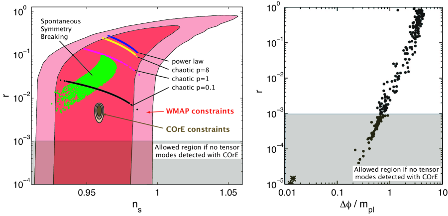
Figure 3: Constraints on inflation from COrE. For a broad range of inflationary models COrE can be expected to detect primordial gravitational waves from inflation. The large contours on the left panel show the present constraints from WMAP seven-year data in the $r$-$n_{S}$ plane. A few parameterized families of inflationary models give an idea of representative model predictions. The small contours illustrate what a COrE detection would look like if $r>5\times 10^{-3}$. The part of parameter space still allowed at 2$\sigma$ in the case of a non-detection is shown in grey. The right panel shows the ‘main sequence’ of inflationary models generated using a model independent approach.

2.1.4 Model independent analysis

One can reformulate the exact dynamical equations for inflation as an infinite hierarchy of flow equations described by the generalized ‘Hubble slow roll’ (HSR) parameters [20, 21, 25, 18, 28, 23, 30]. In the Hamilton-Jacobi formulation of inflationary dynamics, one expresses the Hubble parameter directly as a function of the field $\phi$ rather than a function of time, $H\equiv H(\phi)$ under the assumption that $\phi$ is monotonic in time. Then the equations of motion for the field and background are given by

$$\dot{\phi}=-2M_{\mathrm{Pl}}^{2}H^{\prime}(\phi),\qquad V(\phi)=3M_{\rm Pl}^{2}H(\phi)^{2}-2M_{\rm Pl}^{4}H^{\prime}(\phi)^{2}$$

where the primes denote derivatives with respect to the field $\phi$. The second equation allows us to consider inflation in terms of $H(\phi)$ rather than $V(\phi)$. This approach has the advantage that it allows us to remove the field from the dynamical picture altogether, and study the generic behavior of slow roll inflation without making assumptions about the underlying particle physics (although the underlying assumption of a single order parameter is still present). In terms of the HSR parameters, $\epsilon$ and ${}^{\ell}\lambda_{H}$, the dynamics of inflation is described by the infinite hierarchy

$$\epsilon(\phi)=2M_{\rm Pl}^{2}\left(\frac{H^{\prime}(\phi)}{H(\phi)}\right)^{2}\,,\hskip 28.45274pt^{\ell}\lambda_{H}\equiv\left(2M_{\rm Pl}^{2}\right)^{\ell}\frac{(H^{\prime})^{\ell-1}}{H^{\ell}}\frac{d^{(\ell+1)}H}{d\phi^{(\ell+1)}},\qquad{\rm for}~{}~{}\ell\geq 1.$$ (8)

The flow equations allow us to consider the model space spanned by inflation using Monte Carlo techniques. Since the dynamics is governed by a set of first-order differential equations, one can specify the entire cosmological evolution by choosing values for the slow-roll parameters ${}^{\ell}\lambda_{H}$, which completely specifies the inflationary model. However, in practice one has to truncate the infinite hierarchy at some finite order. We retain terms up to tenth order having checked robustness against the choice of truncation order. We will discuss the meaning and the implications of this truncation below. Moreover, the choice of slow-roll parameters for the Monte Carlo process requires assumptions about priors for the ranges of values taken by the ${}^{\ell}\lambda_{H}$. In the absence of a priori theoretical knowledge about these priors, one can assume flat priors with some ranges dictated by current observational limits, and the requirement that the potential satisfies the slow-roll conditions. Changing this ‘initial metric’ of slow-roll parameters changes the clustering of phase points on the resulting observational plane of a given Monte Carlo simulation. Therefore, the results from these simulations cannot be interpreted in a statistical way. Nevertheless much intuition can be gained from the results of such simulations (e.g., [21, 28, 29]). The simulations show that models do not cover the observable parameter space uniformly but instead cluster around certain attractor regions.

Inflation requires a form of stress-energy which sources a nearly constant Hubble parameter. This can arise via a truly diverse set of mechanisms with disparate phenomenology and varied theoretical motivations. As mentioned above, in the Hubble slow-roll approach it is possible to characterize, in a model independent way, single field models of inflation, including ‘hybrid’ models where, although more than one field is involved, the generation of primordial perturbations is still governed by a single scalar field. This approach has shown [30, 19] that there is a model independent relation between the excursion of the field during inflation ($\Delta\phi$) and the amplitude of tensor modes, a generalization of the well known Lyth bound [27],

$$\frac{\Delta\phi}{M_{\mathrm{Pl}}}\sim\left(\frac{r}{0.01}\right)^{1/2}\hskip 45.52458pt{\rm for}\,\,\,\,\,\frac{\Delta\phi}{M_{\mathrm{Pl}}}\ll 1,$$ (9)

$$\frac{\Delta\phi}{M_{\mathrm{Pl}}}\sim 6.3\,\left(\frac{r}{0.01}\right)^{1/4}\hskip 28.45274pt{\rm for}\,\,\,\,\,\frac{\Delta\phi}{M_{\mathrm{Pl}}}\sim 1.$$ (10)

The second line is a fit to the relation shown in Fig. 3.

The right panel in Fig. 3 shows extracts from a 2 million point Monte Carlo simulation of the inflationary flow equations (adapted from ref. [30]).

While the choice of slow-roll parameters for the Monte-Carlo process requires the assumption of some prior ranges, the results of the simulations do not depend strongly on these choices once known observational constraints (on $n_{S}$ and $dn_{S}/d\ln k$) are imposed. This observation is what makes the conclusions of this section model independent. Note that the simulations show significant concentrations of points with a significant tensor-to-scalar ratio.

From these considerations, it is clear that a value of $r>10^{-3}$ would imply that inflation occurred at energy scales $\gtrsim 2\times 10^{15}$ GeV and that there was a super-Planckian field variation. Therefore $r\sim 10^{-3}$ is a natural target for a CMB polarization experiment. A detection of primordial tensor perturbations $r>10^{-3}$ would probe physics at an energy that is a staggering twelve orders of magnitude larger than the center-of-mass energy at the Large Hadron Collider. Of equal importance is the fact that a detection or constraint on the tensor-to-scalar ratio $r$ at this level will answer a fundamental question about the range $\Delta\phi$ of the scalar field excursion during inflation as compared to the Planck mass scale. This would yield vital clues about physical symmetries at these unexplored energy scales including the ultraviolet completion of gravity.

2.1.5 Forecasts for $r=T/S$

As the foreground signal is expected to dominate the cosmological signal at low $\ell$ at all frequencies, it is of crucial importance to propagate uncertainties connected to foreground contamination into the parameter error forecasts.

An estimate of the error on cosmological parameters in the presence of residual foregrounds is obtained here following the approach proposed in ref. [30] and further developed in ref. [17]. We assume that the knowledge about foreground residuals and their uncertainty is available from estimates obtained by component separation methods as discussed in section 3.4. We assume the same level of foreground residuals for both E and B CMB modes. Component separation residuals in $T$, assumed to be much smaller than the CMB temperature cosmic variance, are neglected here.

Forecasts: method

In refs. [30] and [17] it was assumed that in each frequency band foregrounds could be subtracted down to a certain percentage of the original signal. As this supposes that the level of the foreground contamination after component separation is known a priori, we use here instead the residual foregrounds, uncertainties, and final noise level obtained from cleaning simulated maps of CMB plus Galactic and point source emission, as described in §3.4.

We find that the foreground cleaning approach based on the Needlet ILC (NILC) yields foreground residuals in agreement with the prediction made using the pixel-based linear component separation method (pix-LCS) as described in [228]. This gives us confidence in the validity of the residual foreground estimates.

In the case of a realistic experiment (with partial sky coverage, and noisy data), assuming that CMB multipoles are Gaussian-distributed and that the noise is Gaussian, the likelihood $\cal L$ is given by

$$\frac{-2\ln{\cal L}}{f_{\mathrm{sky}}}=\sum_{\ell}(2\ell+1)\left\{{\rm tr}[\hat{R}_{\ell}R_{\ell}^{-1}]-{\rm ln}\,{\rm det}\,[\hat{R}_{\ell}R_{\ell}^{-1}]-3\right\},$$ (11)

where $R_{\ell}$ is the theoretical multivariate covariance matrix of the $T,E,B$ fields, and $\hat{R}_{\ell}$ its empirical estimate on the observed data. Here $R=C_{th}+N$ where

$$C_{th}=\begin{pmatrix}C_{th}^{TT}&C_{th}^{TE}&0\cr C_{th}^{TE}&C_{th}^{EE}&0\cr 0&0&C_{th}^{BB}\cr\end{pmatrix},\qquad N=\begin{pmatrix}N^{TT}&0&0\cr 0&N^{PP}&0\cr 0&0&N^{PP}\cr\end{pmatrix}$$

and $\hat{R}$ is defined analogously but with $C_{th}$ replaced by $C_{obs}.$ Here $f_{\mathrm{sky}}$ denotes the fraction of sky observed. Note that this accounts for the effective number of modes accessible with partial sky coverage, but does not account for mode correlations introduced by the sky cut, which may smooth power spectrum features. The details of the mode-correlation depend on the specific details of the mask, but for $\ell$ greater than the characteristic size of the survey, our approximation should be valid.

The expression for the likelihood in eqn. (11) with the specified values of $R$ and $\hat{R}$ is valid only for a single frequency experiment. However, cleaning the simulated multi-frequency maps yields (fore each of $T$, $E$ and $B$) a single map of one effective frequency, with an effective noise power spectrum and effective foreground residuals. We express the effect on the power spectrum of the residual Galactic contamination as an additional “noise-like” component, with a dependence on $\ell$ given by the spectral energy distribution of the residual foregrounds. The effective noise also includes a term which is a function of the noise levels of the individual frequency channels. The forecasts are then obtained from the Fisher information matrix (FIM)

$$F_{ij}=-\left.\left\langle\frac{\partial^{2}\ln{\cal L}}{\partial\theta_{i}\partial\theta_{j}}\right\rangle\right|_{\theta=\bar{\theta}}$$ (12)

where the $\theta_{i}$ denote the various model parameters. We then have $\sigma_{\theta_{i}}\geq(F^{-1})_{ii}^{1/2}$ (Cramer-Rao inequality). This becomes an equality for the maximum likelihood estimator in the limit of large data sets, which we assume here. We consider in our analysis the cosmological parameter set

$$\bar{{\bf\theta}}=\{r,n_{S},n_{T},dn_{S}/d\ln k,Z,\Omega_{b}h^{2}\equiv\omega_{b},\Omega_{c}h^{2}\equiv\omega_{c},h,\Omega_{k},A(k_{0})\},$$

where $Z\equiv\exp(-2\tau)$.

Forecasts: results

Table 2 reports the 1$\sigma$ forecast errors on $r$ after marginalizing over the other cosmological parameters, with and without imposing the consistency relation (CR) $r=-8n_{t}$. The $B$ mode polarization signal comes mainly from two regions of the angular power spectrum. At $\ell<20$, the signal comes through the so-called ‘reionization bump’, and there is therefore some sensitivity to the adopted fiducial value for $\tau$. At $\ell>20$ the signal comes from the $BB$ peak, but is contaminated by the lensing signal which depends on the perturbation amplitude, as well as by the instrumental noise, which becomes increasingly important with increasing $\ell$.

parameter	1$\sigma$ error (no CR)	1$\sigma$ error (CR)	$f_{\rm sky}$ used
($r_{\mathrm{fid}}=5\times 10^{-3}$)     $r$	$0.0014$	$6.2\times 10^{-4}$
$n_{S}$	$0.0017$	$0.0017$	70 %
$n_{T}$	$0.12$	N/A
($r_{\mathrm{fid}}=5\times 10^{-3}$)     $r$	$0.0013$	$5.3\times 10^{-4}$
$n_{S}$	$0.0017$	$0.0017$	65 %
$n_{T}$	$0.096$	N/A
($r_{\mathrm{fid}}=1\times 10^{-3}$)     $r$	$0.001$	$5.0\times 10^{-4}$	70 %
($r_{\mathrm{fid}}=1\times 10^{-3}$)     $r$	$7.0\times 10^{-4}$	$2.8\times 10^{-4}$	65 %

Table 2: Forecast errors on $r$ for two fiducial models, assuming foreground residuals as obtained with two independent foreground cleaning methods applied to realistic simulated maps. Results for $r$ are given for two different masks, which correspond to observed sky fractions as listed in the last column.

Fig. 4 shows the joint 1, 2 and 3$\sigma$ regions in the $r$-$n_{S}$ plane, which is relevant for inflationary models. The single field consistency relation has been imposed, and all other cosmological parameters have been marginalized over. Here the result plotted for $r=0.001$ corresponds to the larger mask ($f_{\rm sky}=65$%). Dotted and solid contours for $r=0.005$ show the (small) effect of changing the mask for larger values of $r$, which indicates that the cosmic variance is becoming the major source of uncertainty.

Figure 4: Forecast $1$, $2$ and $3\sigma$ joint constraints in the $r$-$n_{S}$ plane including the effects of foreground subtraction errors. The consistency relation has been imposed. All other cosmological parameters have been marginalized over. The ellipses on the left side correspond to component separation with a large galactic mask blanking out the galaxy at galactic latitudes $|b|\leq 20^{\circ}$ ($f_{\rm sky}=65$%), for $r=0.001$ and $n_{s}=0.96$. Ellipses centered around $r=0.005$ and $n_{s}=0.96$ correspond to a case with five times larger B modes, analyzed with a smaller galactic mask ($f_{\rm sky}=70$%, dotted contours) or with the same mask as in the case $r=0.001$ ($f_{\rm sky}=65$%, solid contours).

The conclusion of the present analysis is that the proposed instrumental setup of COrE will enable us to measure at high statistical significance the target values for $r$ motivated in Sect. 2.1.4 of $r\gtrsim 5\times 10^{-3}$, and to detect $r\sim 1\times 10^{-3}$. This means that it will be possible to explore most large-field models and reach energies $M_{\rm inf}\sim$ few $\times 10^{15}$ GeV.

This analysis can be generalized in the future by using the multi-detector multi component spectral matching independent component analysis (SMICA) [234, 230, 225]. SMICA indeed is a parameter estimation method that uses a multi-detector, multi component extension of the likelihood of eqn. 11, in which a parametric model of theoretical covariances $R(\bar{\theta})$ is matched to measured covariances $\hat{R}$. The approach discussed here is equivalent to the special case of a three-channel SMICA likelihood in which the observations are one map for each of $T,E,B$, the parameters $\bar{\theta}$ are cosmological parameters, and measured covariances $\hat{R}$ comprise a cosmological term as well as a noise term and a foreground residual term (the latter two being assumed to be known). In SMICA, just as here, the final covariance matrix of the parameters of the fit is obtained from the Fischer information matrix. In addition to forecasting the errors (i.e. computing the FIM), SMICA also maximizes the likelihood, using as parameters of the spectral fit not only the set of cosmological parameters, but a set of covariance matrices for various foregrounds. This makes it possible to estimate cosmological parameters directly from the multi-channel data set, while marginalizing over foreground contamination — relaxing the assumption that the exact spectral energy distribution of the residual foreground contamination is known.

This further development will extend on the best of both the method presented here, and the implementation in [225] which assumes cosmological parameters other than $r$ to be known, but unknown foreground residuals. Note that SMICA has “built-in” an estimation of the goodness of fit of the multi-component model of sky emission, is a natural way to handle the problem of estimating the error induced by residual foregrounds.

2.2 Gravitational lensing science

Gravitational lensing of the CMB anisotropies provides a powerful and clean probe of the mass distribution integrated to high redshift. Clustered matter lying between the surface of last scatter and us today distorts the CMB anisotropies by shear and magnification distortions. This is a clean probe because it is the mass that is being probed directly and no complicated astrophysical modelling is required to interpret the data. Moreover since the surface of last scatter is more distant than other objects subjected to gravitational lensing, linear theory (supplemented by small reliable non-linear corrections) suffices to compare observation to theory. The precise determination of the CMB lensing power spectrum with COrE will probe the dark energy sector and measure absolute neutrino masses with a precision not possible with laboratory experiments. In particular, COrE will be able to probe the two hierarchies (‘direct’ and ‘inverted’) suggested by neutrino oscillation experiments.

2.2.1 Physics of CMB lensing

The observed temperature anisotropies and polarization of the CMB are at zeroth order an angular projection of the perturbations to the photons and the spacetime metric around the time of cosmological recombination ($z\approx 1100$). The effect of later cosmic history, and in particular “dark parameters” such as those describing the dark energy and light neutrino masses (much below $1\,\mathrm{eV}$), is only felt through the angular diameter distance to recombination plus small corrections on large angular scales from the late-time decay of gravitational potentials. The dark parameters are therefore largely degenerate in the primary CMB anisotropies.

The degeneracies can be broken with external datasets but also with the CMB itself by exploiting the effect of weak gravitational lensing by large-scale structure on the propagation of CMB photons from recombination to the present. The net deflection, with an r.m.s. of 2.7 arcmin and degree-scale correlations, is a sensitive probe of the growth of structure over a range of redshifts peaking around $z\approx 2$ (see [41] for an extensive review). Lensing has three main effects on the CMB: (i) it blurs out features in the temperature and polarization leading to a smoothing of the acoustic peaks in their power spectra and a transfer of power from large scales into the damping tail on arcminute scales; (ii) it converts $E$-mode polarization into $B$-mode polarization corresponding to an additional white-noise spectrum at the $(5\,\mu\mathrm{K}\,\mathrm{arcmin})^{2}$ level for multipoles $l<300$; and (iii) it generates small levels of non-Gaussianity (in addition to any primordial non-Gaussianity). The latter is easily calculable, and exploiting this non-Gaussianity is key to extracting the lensing information from the observed CMB and to providing a new window for probing the physics of the dark sector.

In essence, a CMB experiment such as COrE with $\mu\mathrm{K}\,\mathrm{arcmin}$ sensitivity and resolution of a few arcmin for the cosmological channels includes a weak-lensing experiment for free. While lensing studies using the CMB have much in common with present and planned surveys of the weak lensing of galaxies, there are important differences. The CMB provides the most distant source plane and so the deflections are larger and are sourced at higher redshift than for galaxy lensing. At higher redshift, the amplitude of the fluctuations is lower and so a wider range of scales can be probed in the linear regime, removing many of the complications of non-linear evolution that complicate galaxy lensing. Moreover, there are no astrophysical issues such as intrinsic alignments of galaxy shapes to worry about. In addition, the statistics of the CMB source plane are well understood so that shear and magnification are equally useful observables. On the downside, the CMB is a single source plane so there is no possibility of performing tomographic studies. Note also that instrumental systematic effects are quite different for the two routes. The different redshift ranges and systematic effects make CMB and galaxy lensing highly complementary, and cross-correlations should be able to provide interesting new results.

2.2.2 Measurement and interpretation of CMB lensing signal

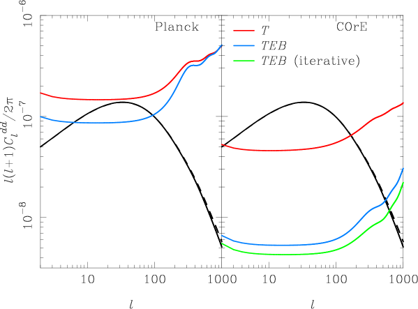
Figure 5: Lensing reconstruction noise on the deflection power spectrum for an extended PLANCK mission (24 months; left) and COrE (right) using temperature alone (red) and temperature and polarization (blue). For COrE, we also show the approximate noise level (green) for an improved iterative version of the reconstruction estimator following Ref. [32]. The deflection power spectrum is also plotted based on the linear matter power spectrum (black solid) and with non-linear corrections (black dashed). The maximum multipole used in the reconstruction is $l_{\mathrm{max}}=2500$.

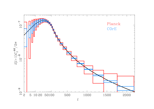
Figure 6: COrE vs PLANCK for measuring the lensing power spectrum. Bandpower errors are plotted (including cosmic variance) on the deflection power spectrum from PLANCK (24 months; red) and COrE (blue) using lens reconstruction with temperature and polarization (no iteration). With COrE, the power spectrum is cosmic-variance limited to $l\approx 500$.

Fixed lenses correlate the observed CMB with the gradient of the unlensed CMB and this property can be used to construct quadratic estimators for the lensing deflection field [36]. Once reconstructed, the deflection field can be used as another cosmological observable. The majority of the information on lensing comes from modes at the resolution limit of the survey so good angular resolution is essential even to reconstruct large-scale lenses. At the WMAP resolution and sensitivity, the reconstruction is very noisy but cross-correlation studies with galaxy surveys have led to a detection at the $3\sigma$ level [38]. A highly significant detection of the deflection power spectrum should be possible with PLANCK’s temperature maps (see Fig. 5 for forecasts) and detailed analysis of the PLANCK maps is underway. Detections are also expected soon from the ground (e.g., with SPT and ACT). However the statistical noise in temperature reconstructions (due to cosmic variance of the primary anisotropies) is such that the deflection power spectrum will only ever be measured to the cosmic variance limit for multipoles $l<100$. To do better, and hence increase the lever arm to constrain dark-sector physics, one must use polarization data. PLANCK is too noisy for polarization to add much, but with COrE it improves the reconstruction greatly; see Figs. 5 and 6. Most of the information comes from the $E$-$B$ correlations and the reconstructed deflection power should be cosmic-variance limited to $l\approx 500$, roughly a 25-fold increase in the number of reconstructed modes with $S/N>1$. Significantly, COrE can mine all of the information in the deflection power spectrum where linear theory is reliable.

2.2.3 Neutrino masses as a unique probe of physics beyond the standard model

There are compelling theoretical reasons why the Standard Model cannot be the last word on particle physics and there are great expectations that the LHC will provide truly telling clues on how the Standard Model should be extended. One area of particle experiment where there has been significant progress towards this goal is exploration of the neutrino sector.

While the Standard Model, as first proposed, implies that there are three exactly massless chiral neutrinos, an abundance of evidence for flavor oscillations has now been accumulated that requires neutrinos to have mass. The most recent data compilations [39] indicate squared mass differences between the three mass eigenstates of $\Delta m_{12}^{2}=(7.59\pm 0.20)\times 10^{-5}\,\mathrm{eV}^{2}$ and $\Delta m_{31}^{2}=\pm(2.43\pm 0.13)\times 10^{-3}\,\mathrm{eV}^{2}$ ($1\sigma$ errors). While the evidence for neutrino mass splittings is overwhelming (the 2002 Nobel Prize in physics was awarded to Davis and Koshiba for this discovery), oscillation experiments are not able to probe the absolute mass scale of the neutrinos. Taking the mass and mixing matrix of charged leptons and quarks as a guide, we would conclude that the most probable values for the neutrino masses would fall into two possible hierarchies: a normal hierarchy with $m_{1},m_{2}\ll m_{3}$ and a total mass close to $0.058\,\mathrm{eV}$; or an inverted hierarchy with $m_{3}\ll m_{1},m_{2}$ and total mass $0.1\,\mathrm{eV}$. However, one should be mindful that neutrinos could well be degenerate with $m_{1}\sim m_{2}\sim m_{3}\gg 0.05\,\mathrm{eV}$.

While laboratory $\beta$-decay experiments can probe absolute masses (or more correctly, effective masses involving the absolute masses and the elements of the electron row of the mixing matrix) the target values for hierarchical masses are well below the detection limit of current and also future experiments. Current searches for neutrinoless double beta decay, which requires massive Majorana neutrinos, limit the effective electron-neutrino mass $m_{\beta\beta}<0.27\,\mathrm{eV}$ (90% confidence) and are complicated by uncertainties in nuclear matrix elements. The other laboratory route uses the kinematical effect of neutrino masses on the extreme tail of the electron energy distribution in ordinary $\beta$ decay. This is challenging due to the very low number of events there. The current upper limit on the effective mass is $m_{\beta}<2\,\mathrm{eV}$ (95% confidence); the KATRIN experiment due to start in 2012 should improve this to $m_{\beta}<0.2$ eV.

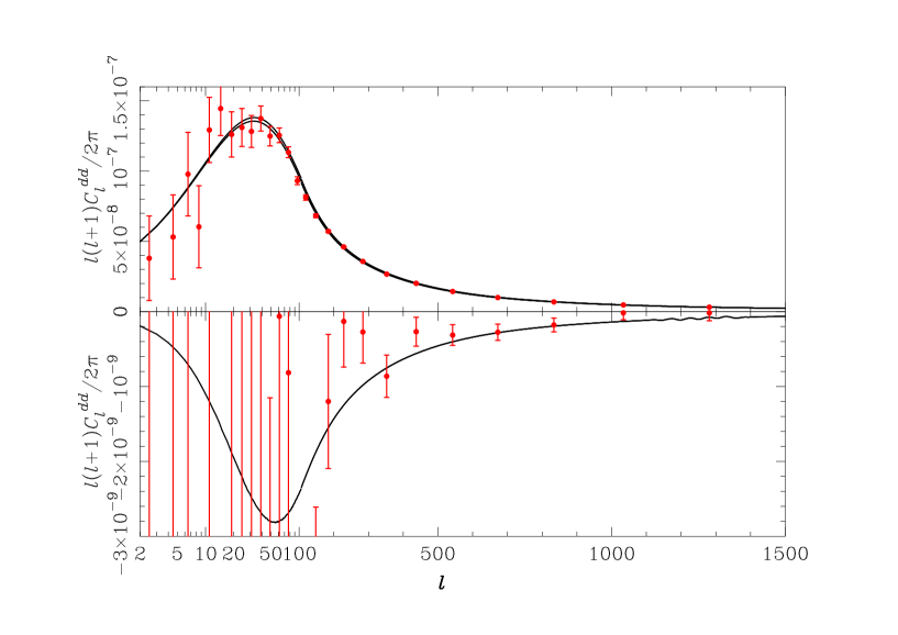
Figure 7: Gravitational lensing deflection power spectrum. The simulated deflection power spectrum from COrE is shown assuming an inverted hierarchy of neutrino masses with the minimum total mass allowed by oscillation data ($m_{1}\approx m_{2}=0.05\,\mathrm{eV}$ and $m_{3}=0\,\mathrm{eV}$). In the upper panel, the solid lines are the theory power spectrum for this scenario (lower) and for three massless neutrinos (upper). The difference between these spectra is plotted in the lower panel illustrating how COrE can distinguish these scenarios from $C_{l}^{dd}$ in the range $l>200$. We have assumed 70% sky coverage after Galactic masking.

Cosmology, however, provides an alternative probe of absolute neutrino masses. Mass splittings from oscillation data imply that at least two mass eigenstates are non-relativistic today. Keeping the densities of all other species (and dark energy) fixed, non-relativistic neutrinos increase the expansion rate at late times over that for massless neutrinos. This impedes the growth of density perturbations on scales small compared to the neutrino free-streaming scale, for which the neutrinos cannot cluster. This mass-dependent suppression of the matter power spectrum on small scales can be measured with CMB lensing even for masses close to the hierarchical targets. We illustrate the capabilities of COrE to distinguish the minimal-mass inverted hierarchy from a model with three massless neutrinos via its reconstruction of the lensing deflection field in Fig. 7. If all other parameters were known, lensing with COrE could constrain the summed neutrino mass to $0.012\,\mathrm{eV}$ (1$\sigma$). However this ignores the issue of uncertainties in the other parameters. While future distance-indicator measurements may help, to be conservative here we consider only constraints from COrE alone in a joint analysis of the unlensed temperature and $E$-mode polarization and the reconstructed deflection field, following [33]. In our MCMC simulations, we vary the standard seven parameters of flat $w$CDM models plus neutrino-mass parameters for three cases. First, we consider a minimal-mass normal hierarchy and use an oscillation prior (ignoring the errors in the squared-mass differences) to fix $m_{2}$ and $m_{3}$ in terms of the lightest mass $m_{1}$ which we allow to vary. Second, we assume a minimal-mass inverted hierarchy and vary $m_{3}$. Finally, we assume degenerate neutrinos and vary the total mass about a model with massless neutrinos. We summarise our results as follows.

• If neutrinos have hierarchical masses, COrE will bound the lightest mass to $m_{1}<0.034\,\mathrm{eV}$ (normal) and $m_{3}<0.045\,\mathrm{eV}$ (inverted) at 95% confidence.

• The minimal-mass inverted hierarchy could be distinguished from a scenario with three massless neutrinos at the $3\sigma$ level.

• If neutrino masses are degenerate, COrE will measure the total mass to $0.03\,\mathrm{eV}$ ($1\sigma$ error). For comparison, the error expected from the Planck nominal mission (including lensing) is $0.10\,\mathrm{eV}$ [33].

Current constraints on neutrino masses from cosmology are rather model dependent and the tightest constraints come from combining multiple datasets (e.g. CMB and large-scale structure data). The 95% limits on the total mass are in the range $0.3$–$2\,\mathrm{eV}$ (see [34] for a recent review). In models in which $w\neq-1$, CMB and large-scale structure data indicate an upper limit at the $1\,\mathrm{eV}$ level. Our forecasted constraints from COrE are for a single homogeneous dataset and are much less model dependent than with current data since the full shape information in the deflection power spectrum is accessible. For example, Ref. [32] show that for a CMB lensing experiment comparable to COrE, there are no significant degeneracies between $\sum_{\nu}m_{\nu}$, $w$ and the spatial curvature. Our constraints from COrE are comparable to forecasts for tomographic studies with future galaxy lensing surveys (assuming a PLANCK prior), for example LSST [35] or Euclid [40], but with quite different systematics.

2.3 Primordial non-Gaussianity

Cosmic microwave background non-Gaussianity is emerging as a powerful new probe of the origin of cosmic structures in the very early Universe and their subsequent evolution (see for example the reviews in [77, 78, 79, 80, 81]). Non-Gaussianity is already the most stringent test of the standard model of inflation, the canonical slow-roll single field model, which predicts negligible primordial non-Gaussianity [86, 85]. The COrE satellite would raise this confrontation to a new level, testing Gaussianity to one part in $10^{5}$. Furthermore, in a complementary way to probing primordial gravitational waves, COrE’s probe of NG offers the prospect of dramatic new insights into fundamental physics and possible signals from the epoch of quantum gravity.

It has often been said that Gaussianity, along with spatial flatness and an approximately scale invariant spectrum of adiabatic cosmological perturbations, is one of the inexorable consequences, or tests, of inflation. While the WMAP data does suggest some hints of non-Gaussianity at low statistical significance, it is remarkable that the primordial signal observed in the CMB turns out to be very nearly Gaussian. Following a series of seminal papers in 2003 where the bispectral non-Gaussianity was calculated for the first time, it was realized that large classes of models predicting measurable non-Gaussianity exist and that CMB constraints of non-Gaussianity are far more robust to foreground systematics than was initially feared (e.g., [109]). Much of the current research in theoretical cosmology has shifted toward exploring what patterns of non-Gaussianity are possible. These possibilities are closely linked to new physics near the Planck scale and modifications of gravity. Conservatively, we estimate that COrE will have a NG discovery potential (defined more quantitatively below) a factor of $\approx 20$ better than PLANCK, approaching the capabilities of an ideal CMB probe.

How does COrE compare to other CMB or non-CMB experiments? An important and unique advantage of COrE over non-CMB probes of NG results from its ability to recognize the distinct patterns which physical mechanisms leave in the shape of higher order correlators, as illustrated in Fig. 8. COrE’s competitive strength will therefore be a vastly enhanced exploration of physically predicted NG shapes compared to any other projected probe of NG. While other probes claim competitive power for detecting ‘local’ bispectral non-Gaussianity (because the effects of nonlinearity can be cleverly factored out for this special case), only the CMB, because of its cleanness and linearity, offers significant sensitivity to other shapes of non-Gaussianity.

Only a high resolution polarization CMB mission such as COrE can provide the high sensitivity for detecting and distinguishing differing NG bispectral shapes. In fact one can show that polarization maps contain more information than temperature maps (although the best constraints arise from combining the two). Polarization is the more powerful probe because the ratio of the expected contaminant signal (mainly galactic dust) to the primordial signal is smaller for polarization than for temperature for the majority of resolved modes. To construct a figure of merit comparing the predicted impact of COrE on physical forms of NG, we compare the predicted constraint volume in bispectrum space spanned by the local, equilateral and flattened bispectra. While PLANCK will reduce the constraint volume by a factor of 70 compared to WMAP, COrE would reduce the volume by another factor of 20. Considering the constraint volume based only on the polarization maps (which provide information independent of the temperature maps and hence provide an important consistency check), we find a volume reduction factor from PLANCK to COrE of order $110$. COrE stands out on account of its full-sky coverage, polarization sensitivity, high resolution, strong rejection of systematics, and the benign environment in space at L2 making COrE the ideal CMB NG probe. On smaller angular scales $(\ell\mathrel{\raise 1.29167pt\hbox{$>$}\mkern-14.0mu\lower 2.58334pt\hbox{$\sim$}}3000)$ the primordial CMB signal becomes subdominant because other highly non-Gaussian compact contaminants (e.g., S-Z clusters and point sources, which are clustered).

The improvement compared with PLANCK will be even more dramatic when considering combined bispectrum and trispectrum constraints on a larger range of NG shapes. The forecast precision with which local trispectrum parameters could be measured with COrE temperature data alone are $\Delta g_{NL}=3\times 10^{4}$ and $\Delta\tau_{NL}=1\times 10^{4}$. COrE’s polarization capability is estimated to sharpen these constraints by a factor of 2. A trispectrum constraint satisfying $\tau_{\rm NL}\ll\frac{1}{2}(6f_{\rm NL}/5)^{2}$ would rule out large classes of multifield inflation models in addition to single field inflation, necessitating a fundamental reassessment of the standard field theory picture of inflation. Beyond searches for primordial NG, COrE will also see NG imprinted on the CMB maps by the lensing/ISW correlation [72, 73, 74]. Such a signal can be exploited to yield the strongest dark energy constraints from the CMB alone. Furthermore, ancillary signatures will constrain modified gravity alternatives to the standard cosmological model.

In addition, there are many alternative inflationary scenarios for which an observable non-Gaussian signal is quite natural, including models with multiple fields, interactions, non-canonical kinetic energy, or remnants of a pre-inflationary phase. There are also more exotic paradigms which can create NG such as cosmic (super-)strings [82, 83] or a contracting phase with a subsequent bounce [84]. Each of these scenarios leaves a distinct NG fingerprint, essentially the ‘shape’ of the higher order correlators. This fingerprint can discriminate between many different inflationary models which are indistinguishable based on the the CMB power spectra alone. It can also be robustly distinguished from astrophysical NG fingerprints left by weak lensing, extra-galactic and galactic astrophysical signals that are interesting in their own right, and spurious NG fingerprints due to instrumental noise.

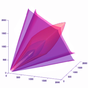
Figure 8: Theoretical predictions for CMB bispectrum shape. The primordial CMB bispectrum depends on three multipole numbers $\ell_{1},\ell_{2},\ell_{3}$ subject to a triangle inequality constraint as opposed to the standard ‘Gaussian’ power spectrum $P(\ell)$ (which depends on only one multipole number). Hence the bispectrum contains rich shape information that can be exploited to confront observations with theoretical models and to probe the self-consistency of a possible detection. Here the CMB bispectra $B(\ell_{1},\ell_{2},\ell_{3})$ from three theoretical models are plotted with positive (cyan) and negative (magenta) isocontours [111, 83]. The plots show (from left to right) the ‘local’ model (e.g., multifield inflation), equilateral model (e.g., DBI inflation) and non-Gaussianity generated by cosmic strings, which are inherently highly nonlinear.

Non-Gaussianity is typically characterized by the parameter $f_{\rm NL}$, which is the amplitude of three-point correlations for the so-called ‘local’ model (the best-motivated case which we will describe below). The equivalent amplitude parameters for the local four-point correlations or trispectrum are $g_{\rm NL}$ and $\tau_{\rm NL}$ (for single-field inflation, we have $\tau_{\rm NL}=(6f_{\rm NL}/5)^{2}$). Inflation predicts negligible primordial NG ($f_{\rm NL}\ll 1$) if the following minimal conditions are satisfied [87]: i) a single field is responsible for driving inflation and generating the quantum fluctuations which are stretched on superhorizon scales to become the seeds for structure formation; ii) such a field has canonical kinetic energy so that its fluctuations propagate at the speed of light; iii) the inflaton obeys slow-roll, that is, it evolves slowly relative to the Hubble timescale; iv) all pre-inflationary state information has been erased during inflation. The violation of any of the above conditions can lead to the generation of a large detectable non-Gaussian signal. Each physical effect leaves its own recognizable fingerprint (see Fig. 8).

Models with field interactions generate ‘local’ primordial NG, which peaks in ‘squeezed’ triangles (see, e.g., [102, 103, 104, 105]); models with non-canonical kinetic term [90] (as, e.g., DBI  [91] and ghost inflation [92]) generate ‘equilateral’ NG, while trans-Planckian effects generate NG which peaks for ‘folded/flattened’ triangles; inflationary models violating slow-roll can generate more complicated shapes (see, e.g.,  [95, 96, 97]). A linear combination of these shapes can also be realized [93]. All these models can naturally predict values of $f_{\rm NL}\gg 1$.

Whether the different shapes are observationally distinguishable can be determined by their cross-correlations, reducing the search categories [111]. Important tests of inflation include the following:

• A detection of any such primordial signal would rule out all standard slow-roll models of single-field inflation.

• Even more striking is the fact that a detection of local non-Gaussianity would rule out all classes of single-field (slow-roll) inflationary models irrespective of their Lagrangian. [99].

• A significant trispectrum measurement satisfying $\tau_{NL}\ll\frac{1}{2}\left(6f_{NL}/5\right)^{2}$ would rule out standard multifield inflation [208, 209, 76].

Beyond these special cases, general estimators have now been developed to search efficiently for arbitrary shapes in the CMB data, allowing any model or mechanism to be directly tested [113]. Another testable prediction of various non-standard models of inflation is that the non-linearity parameter $f_{\rm NL}$ can have a significant scale dependence, parameterized in terms of a running NG index $n_{\rm NG}$ as $f_{\rm NL}=f_{\rm NL}(k)(k/k_{*})^{n_{\rm NG}}$ (see, e.g. [100, 90, 101, 105, 106, 107]).

There are also models with a negligible bispectrum and a large trispectrum, including inflation with a parity symmetry [94, 75] and cosmic strings [83]. In the latter case, it is clear that the trispectrum will provide a significantly stronger constraint on the string tension than the power spectrum or bispectrum [83], though it will also be efficient to search for cosmic defects NG using other specially tailored methods or templates [82].

What if there is no detection of primordial NG? In this case COrE would rule out all scenarios whose natural parameter space result in high values of the NG parameters such as $f_{\rm NL}$, while rendering many other early universe mechanisms cosmologically irrelevant. Examples include DBI inflation models typically predicting $|f_{\rm NL}|>5$ and competitors to inflation like ekpyrotic/cyclic models predicting measurable $|f_{\rm NL}|\sim 10$ [108].

NG from anisotropic cosmologies and topology: Deviations from isotropy as suggested by analyses of the WMAP temperature signal will be confirmed or otherwise by PLANCK but COrE will add the unambiguous consistency check of measuring the presence or otherwise of the corresponding signal in polarization, which could reflect the presence of anisotropy during inflation itself. Moreover, the polarization signature of simply-connected topologies will be stronger than for temperature, in contrast to the situation for PLANCK and WMAP where it is undetectable.

‘Agnostic’ NG searches: The much larger number of resolved modes in the COrE data allows detailed model-independent searches for anomalies in the temperature and polarization maps, which may signal new physics. The addition of high signal-to-noise polarization information with COrE allows for significant cross-checks since any model explanations of candidate anomalies seen in temperature data can be checked against the polarization data COrE will provide. This redundancy will offer significant discovery potential for relics of physics beyond the standard model of cosmology in the early universe.

2.4 Other cosmology

2.4.1 Parameters

Although in the previous sections we have highlighted three key areas—primordial gravitational waves from inflation, gravitational lensing science, and non-Gaussianity searches— as the mainstays of the cosmology part of the COrE science program, because of the leap in sensitivity afforded by COrE, a host of other cosmology projects will be made possible and the potential for serendipitous discoveries is very high. To quantify this potential, we stress that COrE will:

• Map the B mode polarization with $(S/N)\approx O(1)$ up to $\ell\mathrel{\raise 1.29167pt\hbox{$<$}\mkern-14.0mu\lower 2.58334pt\hbox{$\sim$}}100$ no matter how small $r$ is, owing to the gravitational lensing signal, which is essentially guaranteed.

• Map the E mode polarization at the cosmic variance limit for $\ell\mathrel{\raise 1.29167pt\hbox{$<$}\mkern-14.0mu\lower 2.58334pt\hbox{$\sim$}}2000$ at $(S/N)\gg 1.$ By contrast PLANCK measures the E mode with S/N oscillating near one up to $\ell\mathrel{\raise 1.29167pt\hbox{$<$}\mkern-14.0mu\lower 2.58334pt\hbox{$\sim$}}800$.

• Map the T anisotropy at the cosmic variance limit for $\ell\mathrel{\raise 1.29167pt\hbox{$<$}\mkern-14.0mu\lower 2.58334pt\hbox{$\sim$}}2000$ and measure the TT power spectrum up to $\ell=3000.$ (By contrast the PLANCK T measurement is cosmic variance limited only up to $\ell\mathrel{\raise 1.29167pt\hbox{$<$}\mkern-14.0mu\lower 2.58334pt\hbox{$\sim$}}1200$.)

This massive increase in precision will allow the cosmological parameters of a vanilla minimal cosmological model to be determined approximately 2–3 better than possible with PLANCK and will probe with high precision the consistency of the temperature and polarization anisotropies. Moreover, using the COrE data, many extensions of the standard cosmological model including possible new physics will become testable within the interesting range for the new parameters. One possible and not at all unlikely outcome is that thanks to this increased precision we might have to abandon the vanilla model and we could see the “concordance” unravel.

Since it is not possible to enumerate all the non-minimal models that could be tested, to illustrate the potential, we present results for the improvement in the determination of the minimal cosmological parameters as well as two example of extensions showing how the limits would improve with the COrE relative to PLANCK. Table 3 shows the forecast for the constraints on the parameters of a “minimal” cosmological model described by the cosmological parameters:

$$\omega_{b},~{}~{}\omega_{c},~{}~{}\Theta_{s},~{}~{}n_{s},~{}~{}\log[10^{10}A_{s}]$$ (13)

where $\omega_{b}\equiv\Omega_{b}h^{2},$ $\omega_{c}\equiv\Omega_{c}h^{2}$ are the physical baryon and cold dark matter densities relative to the critical density, $\Theta_{s}$ is the ratio of the sound horizon to the angular diameter distance at decoupling, $A_{s}$ is the amplitude of the primordial spectrum, and $n_{s}$ is the scalar spectral index. The forecasts were computed using an MCMC approach as described in Galli et al. (2010) and the COrE experimental specifications given previously. Together with the standard deviations on each parameter, we also report the improvement factor for each parameter defined as the ratio $\sigma_{\rm Planck}/\sigma_{\rm COrE}$. The values in the Table show that the COrE satellite will improve by a factor $\sim 3$ the constraints on the baryon density, $H_{0}$ and $\theta_{s}$, while the constraints on parameters such as $n_{s}$ and $\tau$ are improved by a factor $\sim 2$.

We have also considered a model with an extra background of relativistic non-interacting particles, $N^{\rm eff}_{\nu}$ and a model in which the Helium abundance $Y_{p}$ is allowed to vary. COrE will improve the constraints on these parameters by a factor of $\sim 3$ with respect to PLANCK.

Parameter
uncertainty	Planck	COrE		Planck	COrE		Planck	COrE
$\sigma(\Omega_{b}h^{2})$	0.00011	0.000034	(3.3)	0.00017	0.000049	(3.6)	0.00016	0.000048	(3.3)
$\sigma(\Omega_{c}h^{2})$	0.00087	0.00037	(2.4)	0.0022	0.00073	(3.1)	0.0009	0.00036	(2.5)
$\sigma(H_{0})$	0.0039	0.0014	(2.8)	0.011	0.0034	(3.3)	0.0046	0.0016	(3.1)
$\sigma(\tau)$	0.0040	0.0022	(1.8)	0.004	0.0022	(1.8)	0.0040	0.0023	(1.8)
$\sigma(n_{s})$	0.0027	0.0014	(1.9)	0.0056	0.0025	(2.3)	0.0053	0.0024	(2.3)
$\sigma(10^{10}A_{s})$	0.18	0.10	(1.8)	0.23	0.11	(2.1)	0.19	0.10	(1.9)
$\sigma(N_{\rm eff})$	$-$	$-$	$-$	0.14	0.044	(3.3)	$-$	$-$	$-$
$\sigma(Y_{p})$	$-$	$-$	$-$	$-$	$-$	$-$	0.0083	0.0027	(3.1)

Table 3: Improvement of CORE relative to PLANCK on measuring cosmological parameters. $1\sigma$ errors on cosmological parameters. In parenthesis we give the improvement factor in the confidence level for the corresponding COrE configuration with respect to PLANCK. The second set of columns correspond to the case of an extra background of relativistic particles $N_{\rm eff}$. The third set of columns consider variations in the primordial ⁴He fraction abundance, $Y_{p}={}^{4}{\rm He}/(H+{}^{4}{\rm He})$.

COrE will provide valuable constraints on the physics of the neutrino decoupling from the photon-baryon primordial plasma. As it is well known, the standard value of neutrino parameters $N_{eff}=3$ should be increased to $N_{eff}=3.04$ due to an additional contribution from a partial heating of neutrinos during the electron-positron annihilations. This effect, expected from standard physics, can be tested by the COrE experiment, albeit at just one standard deviation. However, the presence of nonstandard neutrino-electron interactions (NSI) may enhance the entropy transfer from electron-positron pairs into neutrinos instead of photons, up to a value of $N_{eff}\sim 3.15$. This value would be distinguished by COrE from $N_{eff}=3$ at $\sim 3$, shedding new light on NSI models.

COrE will also provide an independent determination of the primordial Helium abundance. Current astrophysical measurements of primordial Helium converge towards a conservative estimate of $Y_{p}=0.250\pm 0.003$. Table  3 shows that the COrE experiment will reach a precision comparable to current astrophysical measurements, opening a new window for testing systematics in current primordial helium determinations and further testing Big Bang Nucleosynthesis.

COrE will also be able to test the adiabaticity of the primordial scalar perturbation by probing for the presence of isocurvature perturbations of various types. (See for example [188, 189] and references therein.) This is an important point because although the simplest possibility is that the perturbations were completely adiabatic, a myriad of models have been proposed that include some degree of isocurvature perturbations as well and the only way to rule out these models is through better observations [191, 192, 193]. COrE will improve constraints on isocurvature perturbations to the total CMB power spectrum. Considering a generic cosmological model with the addition of CDM, neutrino density and neutrino velocity isocurvature modes, a Fisher forecast of COrE shows an improvement of these constraints by approximately a factor of two over PLANCK. The most improved constraints will be those on the contribution of the neutrino density and velocity isocurvatures, which will be more than double that of PLANCK [190].

2.4.2 Reionization history of the Universe

One of the most striking contributions of the WMAP space mission was its measurement of the reionization optical depth $\tau$ of the microwave photons through its characterization of the E mode polarization on very large angular scales. According to the seven-year WMAP analysis [163], the current uncertainty on $\tau$ is $\simeq\pm 0.015$, almost independently on the specific model considered. Under various hypotheses (simple $\Lambda$CDM model with six parameters, inclusion of curvature and dark energy, of different kinds of isocurvature modes, of neutrino properties, of primordial helium mass fraction, or of a re-ionization width) the best fit of $\tau$ lies in the range 0.086–0.089. On the other hand, allowing for the presence of primordial tensor perturbations or (and) of a running in the power spectrum of primordial perturbations the best fit of $\tau$ goes to 0.091–0.092 (0.096). PLANCK will certainly put new light on this topic thanks to its high sensitivity to E mode polarization, but this underlines the relevance of carrying out a combined analysis of the re-ionization of the Universe and of primordial tensor perturbations, firmly possible only through high accuracy measurements of both E and B modes. Re-ionization results from ionizing radiation emitted by very first structures formed in the high-redshift Universe – either by very massive stars or by quasars – and a better characterization of the full re-ionization history as a function of redshift would provide important clues for understanding the scenarios of structure formation and radiative feedback processes [164] resulting in a different suppression of star formation in low-mass haloes. The precise polarization data that COrE will provide at very low multipoles will be invaluable to this endeavor. The principal component analysis can be used to provide model-independent constraints on the re-ionization history of the Universe [165] from CMB polarization data at low multipoles. Furthermore, the COrE resolution up to a few arcminutes will constrain alternative (double-peaked or very high redshift) re-ionization models, invoking non-standard processes such as evaporation of mini-blackholes or particle decays and annihilations, manifesting themselves also at high multipoles [166]. Moreover, COrE will measure and constrain models of patchy reionization and probe parameters such as the duration of the patchy epoch and the mean bubble radius [167].

2.4.3 Primordial magnetic fields

Synchrotron emission and Faraday rotation measurements provide increasing evidence that the large scale structures in the Universe, such as galaxies and clusters, are pervaded by magnetic fields which are of order a few micro-Gauss. An open question is whether these fields were seeded in the Early Universe (by fields of a few nano-Gauss that arise in inflation or cosmological phase transitions) or whether they originated later on through astrophysical processes. In either case they would have sourced CMB anisotropies leading to unique observational signatures. Very large scale, quasi-homogeneous magnetic fields lead to very distinct cross correlations between E and B modes. Smaller scale, stochastic magnetic fields lead to a characteristic peak in the B-mode power spectrum at $\ell\sim 2000$. COrE will detect magnetic fields at the sub nano-Gauss level permitting an accurate characterization of their origin and evolution.

2.4.4 Topological defects

One view of the Early Universe is that the fundamental interactions are unified at some high energy scale, typically presumed to be Grand Unified Theory (GUT) energy scale $\eta\sim 10^{16}\,{\rm GeV}$, where there exists a symmetry connecting the electromagnetic, weak nuclear and strong nuclear forces. Evidence for this comes from the running of the couplings of the individual interactions with energy and the fact that the Electroweak Symmetry forms the basis of the standard model. This symmetry would be broken at phase transitions during the Early Universe and topological defects can form when the topology of the vacuum manifold is non-trivial. This is likely to be the case for a large fraction of symmetry breaking schemes from popular GUT models such as $SO(10)$ [42].

An alternative is that the fundamental interactions are unified in String Theory, which is self-consistent only when the number spatial dimensions is much higher than the standard 3, typically 10 or 11 in the most popular models. Such models allow for a plethora of higher-dimensional topological defects known as D-branes, which can behave like cosmic strings from the three-dimensional point of view [45]. These cosmic superstrings [46] exhibit a range of complicated dynamics such as multiple tension networks that are the subject of on-going investigations.

A number of inflationary models derived from fundamental physics lead to the formation of topological defects at the end of inflation. Such models are known as hybrid inflation models [43, 44]. Since the energy scale associated with these models is typically the GUT scale, the topological defects lead to potentially detectable signatures uncorrelated with those from inflation. These include superymmetric (SUSY) hybrid inflation [47, 48] and brane inflation [49]. In both cases, and possibly more generally, the inflation generated gravitational wave background will be undetectable, $r\ll 10^{-4}$, in such models, but there will still be a B-mode signature produced by the defects [50, 51, 52, 53, 54] because defects produce significant levels of vector modes. Moreover, non-topological defects from global O(N) symmetry breaking at the end of inflation can generate a scale-invariant spectrum of GWs with an amplitude significantly larger than that from inflation [55, 56].

The most commonly studied models are cosmic strings, which might be formed, for example, if the symmetry breaking transition results from the breaking of a $U(1)$ symmetry. The amplitude of the anisotropies and polarization for the CMB (and all other gravitational effects) created by strings is governed by the dimensionless parameter $G\mu/c^{2}.$ $\mu\sim\eta^{2}$ is the mass per unit length of the strings. For a symmetry breaking transition that takes place at $\eta$, we find that $\mu\sim\eta^{2}.$ $G\mu/c^{2}$ is typically $\sim 10^{-6}$ for strings formed at the GUT scale. The zoo of possible topological defects models is large and includes textures [57], semi-local strings [58] and strings with multiple tensions motivated by cosmic superstrings [59]. The spectra for these models are qualitatively similar to those for strings and therefore we will concentrate specifically on strings.

There is some uncertainty in precise details of the anisotropies and polarization predicted by cosmic strings [60, 61, 62, 63, 64, 65, 66]. The qualitative features of the anisotropy spectrum $(\Delta T_{\ell})^{2}=\ell(\ell+1)C_{\ell}/2\pi$ are: (i) a gradual increase at low- $\ell$, due to the Integrated Sachs-Wolfe (ISW) effect from strings along the line of sight, to a peak somewhere between $\ell=500$ and 800—the precise scale being set by the correlation length of the network; (ii) a significant contribution from vector modes due to the large velocity component of the energy-momentum tensor and no Doppler peaks due to the lack of coherence of the perturbations; (iii) a power law (as opposed to exponential) decay which results from sharp features induced by the Kaiser-Stebbins effect [194]. The E-mode polarization spectrum is similar to the anisotropy spectrum, although it lacks the ISW contribution on large and small scales.

The B-mode power spectrum from strings is very different to that due to inflation induced gravitational waves. The spectra predicted by Abelian-Higgs (AH) simulations and Nambu simulations created using the ‘unconnected segment model’ (USM) are presented in Fig. 9 with their amplitude set by the upper limits on $G\mu/c^{2}$ as discussed in the next paragraph. The qualitative features of the string and inflationary spectra are quite similar but the precise scales involved are very different. See ref. [64] for a discussion of the differences between these two possible manifestations of the spectrum. On large scales there is a bump at low $\ell$ due to reionization and then there is an approximately white-noise ($C_{\ell}$ constant) portion of the spectrum rising to a peak. However, the peak is somewhere between $\ell=500$ and 1000 for strings, in contrast to $\ell\sim 100$ expected for inflationary spectra. The reason why the peak is at higher $\ell$ is because the defect models create perturbations inside the horizon as opposed to at horizon crossing, which is the case in inflationary models. Unfortunately, there is some disagreement over the precise value of the correlation length and this leads uncertainty in the peak position. There are no peaks in the high $\ell$ power spectrum. The spectrum due to strings is, in fact, very similar to that created by gravitational lensing of density perturbations and they could easily be confused, particular for the case of the Nambu spectrum.

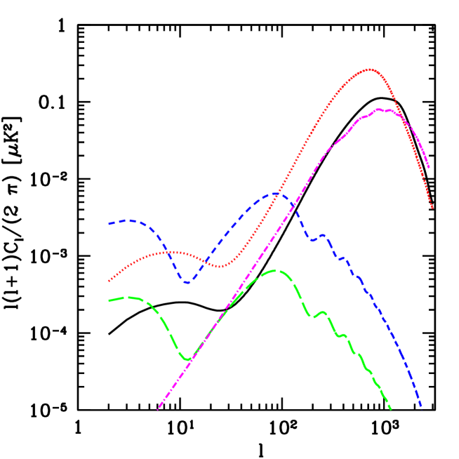
Figure 9: $B-$mode polarization power spectra from strings, tensors and gravitational lensing presented in ref. [64]. For the string spectra, we use values of $G\mu/c^{2}$ corresponding to the $2\sigma$ upper limit from CMB+SDSS data, that is. $G\mu/c^{2}=2.6\times 10^{-7}$ for the USM Nambu model (solid) and $6.4\times 10^{-7}$ for the USM AH case (dotted). We also show the inflationary primordial tensor spectrum with $r=0.1$ at $k=0.05\,{\rm Mpc}^{-1}$ (short dashed) and $r=0.01$ (long dashed). Finally, we show the gravitational lensing spectrum generated from $E-$mode mixing (dot-dash) expected in the inflationary model.

The present $95\%$ upper limits on $G\mu/c^{2}$ come from a fit to the standard six parameters plus an additional parameter to describe the amplitude of the string spectrum which is usually $G\mu/c^{2}$ or $f_{10}$, the contribution of strings to the $\ell=10$ multipole. Using properties of the string networks computed in Nambu simulations in the USM one finds that $G\mu/c^{2}<2.6\times 10^{-7}$ [64] using WMAP and SDSS and this can be improved to $1.6\times 10^{-7}$ [67] using results from ACT, whereas if one uses the spectra computed directly from Abelian Higgs simulations one finds that $G\mu/c^{2}<7\times 10^{-7}$ [62] using just WMAP. In addition there is an even less certain limit of $G\mu/c^{2}<7\times 10^{-7}$ from the absence of a stochastic gravitational wave background created by the decay of cosmic strings loops [64].

We have performed an analysis of the prospects for detecting this background using COrE following the methods recently used for simulated CMBPOL observations [68]. We simulate CMB data for a flat $\Lambda$CDM model with the set of parameters used in ref. [69] and foreground subtraction residuals are also included [70] with the aim of propagating their effect into parameter uncertainties. We use the cosmic variance of the weak lensing B-mode signal as additional uncertainty on the B-mode spectrum. We use the string B-mode spectrum computed directly from the AH simulations. We assume the inflationary consistency relation $n_{\rm t}=-r/8$ for the tensor spectral index and do not allow running of the scalar spectral index. The inflationary parameters are specified at a pivot scale of $k_{*}=0.05\,{\rm Mpc}^{-1}$. We assume that 80% of the sky can be used for cosmological analysis. The simulated data with noise expected for COrE are used as an input to MCMC analysis using COSMOMC [71].

In an 9 parameter fit (the standard 6 parameters plus $r$ and the amplitudes of a string and texture components, for a model with no inflationary induced gravitational waves nor any defect component, we find limits $r<10^{-3}$, $f_{10}^{\rm str}<1\times 10^{-4}$ and $f_{10}^{\rm tex}<5\times 10^{-4}$ where $f_{10}^{\rm str}$ and $f_{10}^{\rm tex}$ are the contributions of the strings and textures to the anisotropy power spectrum at $\ell=10$ respectively. The correlation between tensors and strings is small, and there is little chance of signal misidentification (the quality of the fits, i.e., mean or best-fit likelihoods would point to the right component). A Bayesian model selection analysis that takes model priors into account will also be feasible to address model-level questions on the evidence for various defects, as demonstrated in ref. [68]. In absence of a detection COrE will deliver simultaneous 95% confidence upper limits of $1\times 10^{-3}$ on tensors and $6\times 10^{-8}$ on the $G\mu/c^{2}$ of strings compared to the present limit which is $7\times 10^{-7}$ for this model. Similar detection opportunities apply to other defect models such as textures and the fact that the different components are uncorrelated means that one can not just to detect defects, but to distinguish the type of symmetry breaking pattern through the type of defects generated. This would be an entirely unique measurement.

2.5 Galactic science

Undoubtedly, any claim of a detection of B-mode CMB polarization will face a critical assessment against alternative interpretations involving foreground contributions. The necessity of reliable foreground removal links the search for a polarization signal from cosmic inflation to research in Galactic astrophysics. Converserly, COrE hold promises of breakthroughs in our understanding of the dusty magnetized interstellar medium in the Milky Way.

Dust and synchrotron radiation from the Galaxy are the dominant contributions to the microwave sky polarization. Synchrotron radiation traces the magnetic field over the whole volume of the Galaxy, while dust polarization traces the field within interstellar clouds. COrE will image these two complementary tracers of the Galactic magnetic field with the sensitivity and angular resolution needed to gain a complete view of Galactic magnetism. The improvement in sensitivity of COrE over Planck is factor of 10 for the dust polarization and a factor of 30 for the synchrotron emission. At the highest frequency COrE will map the field with an angular resolution of 1.3’, a factor 3 better than Planck, which complements the small angular scales probed with ground based instruments. This quantitative jump forward in the observations will provide the missing data needed to map continuously the Galactic magnetic field. The data analysis will unravel the interplay between the magnetic field and interstellar turbulence, and the role that the field plays in the formation of interstellar structure and star formation. COrE polarization observations will provide complementary information to advance our understanding of the nature of interstellar dust, its evolution across interstellar space, and grain alignment with the field direction.

2.5.1 Galactic magnetic field

The Galactic ecological system cannot be understood without knowledge about the strength and structure of its magnetic field. COrE will make possible to understand this elusive but dynamically important component of galaxies.

The magnetic field is dynamically tied to cosmic rays and the turbulent interstellar gas. These three components have comparable energy densities indicating that they are in continuous interaction and providing feedback to each other. The importance of the magnetic field for the energetics of the interstellar medium (ISM), star formation, and galaxy evolution is widely recognized, but its actual role remains quantitatively debated due to the paucity of data on its its correlation with interstellar turbulence and the density structure of the ISM. We detail some of the prime questions that the COrE data will resolve in a unique way.

(1) What is the impact of the magnetic field on the interstellar medium energetics?

Synchrotron emission is a prime tracer of the galactic magnetic field. The synchrotron intensity allows estimation of the total magnetic field strength, while its polarization fraction gives information about the field structure on both global and local scales. The COrE sensitivity will be far superior to other missions. It will provide a major step forward in our ability to study magnetic fields in the Milky Way disk and halo. The very accurate, highly resolved and detailed view at the polarization of synchrotron emission will be free of Faraday rotation. Faraday rotation causes the synchrotron polarization vector to turn as it propagates through the magneto-ionized medium. This greatly complicates analyzing synchrotron emission and can lead to depolarization. At COrE frequencies, the observed polarization angle of the synchrotron emission directly relates to the direction of the magnetic field at the location of emission. This gives a diagnostic of the Galactic magnetic field complementary to ground-based observations at lower frequencies subject to significant Faraday rotation.

Fluctuations in the synchrotron flux in intensity and polarization provide insight into magnetic turbulence. Several characteristic statistical properties are encoded in these data, for example the magnetic energy and helicity spectra as well as the spectrum of the magnetic tension force. The accuracy of the COrE data will thus provide a unique opportunity to study magneto-hydrodynamical turbulence and dynamo action, which govern magnetic field amplification and the energetics of the ISM. It will drastically increase the spectral range of accurately probed magneto-hydrodynamical modes. Therefore the detection potential for relevant plasma physics processes and their characteristic scales such as turbulent energy injection and dissipation will be considerably increased.

(2) What role does the magnetic field play in the evolution and structuring of interstellar matter and the onset of star formation?

The interplay between turbulence and magnetic fields is also key to star formation. To investigate this question one needs to study the polarization of the dust emission, which traces the magnetic fields within interstellar clouds. Dust polarimetry in emission traces the interstellar magnetic field projected on the plane of the sky. It is possible to estimate the magnetic field intensity from polarimetric maps by relating the local dispersion of polarization angles and the local amplitude of the turbulent gas motions, a method first proposed by [155].

The COrE survey will provide the combination of sensitivity and angular resolution required to map continuously the Galactic magnetic field associated with interstellar matter, from the diffuse interstellar medium to molecular clouds where pre-stellar cores are formed. No other experiment offers such a capability. Planck data will provide much information on the Galactic magnetic field on large scales, but does not have the required sensitivity to map the field across the diffuse interstellar medium. Nor do upcoming balloon-borne experiments such as Polar-BLAST and PILOT have the required sensitivity. Stellar polarization observations will continue to improve, but they are intrinsically limited to discrete sets of sight lines. Ground based telescopes at sub-mm and millimeter wavelengths including ALMA will image at sub-arcminute angular scales a variety of compact sources including pre-stellar condensations, but they cannot map polarization from diffuse emission.

Star formation occurs as a result of the action of gravity, which is counteracted by thermal, magnetic and turbulent pressures ([161] and [162]). In the diffuse interstellar medium, outside star-forming molecular clouds, the kinetic energy from interstellar turbulence and the magnetic energy are comparable. Both are much larger than the cloud gravitational binding energy and the gas internal energy. For stars to form, gravity must become, locally at least, the dominant force. This occurs where the turbulent energy has dissipated and matter has condensed without increasing the magnetic field flux in comparable proportions. When and how frequently does this occur? This question is key to our physical understanding of what regulates the efficiency of star formation. There is a broad consensus that the answer will follow once we have a physical understanding of the interplay between interstellar turbulence and the magnetic field structure in interstellar clouds.

The consumption timescale of the molecular gas in the Milky Way, $\rm\sim 10^{9}\,yr$, is two orders of magnitude larger than the dynamical timescale of its giant molecular clouds (i.e., their cloud crossing time). The explanation of this observational fact, established in the early 80s with the advent of CO observations, is still a subject of debate. The first scenario proposed to regulate star formation combines long cloud lifetimes and a low star formation efficiency. According to this scenario, molecular clouds are prevented from collapsing on large scales by turbulent and magnetic pressures, while star formation is locally controlled by the rate at which material can cross field lines through ambipolar diffusion. Observations and numerical simulations are challenging this view ([154]). It is increasingly believed, but still debated, that the bottle-neck to star formation is the formation of magnetically supercritical condensations where the magnetic pressure is too weak to counteract gravity. Once formed, these condensations rapidly collapse to form stars. Star formation would generally be inefficient, because only a small fraction of the matter reaches this stage within a cloud lifetime. Under this second paradigm, molecular clouds are transient, and dynamically evolving gas concentrations are produced by compressive motions out of diffuse interstellar matter. This view stresses the importance of the unique ability of the COrE survey to map the field structure over the extended regions of molecular clouds and of the diffuse interstellar medium. COrE will provide the missing observations that we need to understand how the interplay between turbulence and magnetic fields determines the initial conditions for star formation within the diffuse interstellar medium.

(3) What is the impact of the magnetic field on the large-scale structure and evolution of the Galaxy?

COrE is expected to provide important new clues concerning the effects of the Galactic magnetic field on larger scales. We know that the magnetic field helps support the interstellar gas against its own weight in the Galactic gravitational potential and that it confines cosmic rays to the Galactic disk. In this manner, both the magnetic field and cosmic rays partake in the overall hydrostatic balance of the interstellar medium, causing the gaseous disk to become much thicker. In turn, the thickening of the disk tends to make it unstable to the Parker instability (a type of magnetic Rayleigh-Taylor instability). As this instability develops, magnetic field lines undulate, and the interstellar gas slides down along the field lines into the magnetic troughs accumulating there. The whole process, it has been suggested, could give birth to new molecular cloud complexes and ultimately trigger star formation.

The magnetic field is also believed to play an important role in disk-halo interactions, although the exact mechanisms involved are still poorly understood and debated. A priori one expects the magnetic field to impede mass exchange between the disk and the halo. The magnetic field could tend to contain super-bubbles and prevent them from venting their gas into the halo. This view is challenged by observations of edge-on galaxies which show evidence for a multiphase halo in galaxies like the Milky Way (e.g., NGC 4631 [207]). In contrast to previous studies that used a static medium, numerical simulations that follow the evolution of superbubbles within a supernova-driven turbulent magnetized medium suggest that blowout is more likely than previously thought, mainly because bubbles evolve in an inhomogeneous background medium [205]. Theoretical studies also suggest that the magnetic field might stabilize infalling clouds and enable them to reach the disk without being disrupted by their dynamical interaction with the hot halo gas [206]. To test these ideas and numerical simulations, it is crucial to gain a better observational knowledge of the Galactic magnetic field, particularly in the halo. Similarly, a better knowledge of the Galactic magnetic field, both in the disk and in the halo, will make it possible to place stronger constraints on the existing dynamo scenarios.

2.5.2 Polarization properties of interstellar dust

The unique combination of spectral and spatial information provided by the COrE survey will open a new dimension to our understanding of dust, its nature, and its evolution within interstellar space.

The Galactic interstellar medium is dusty. Large dust grains (size $>10$ nm) dominate the dust mass. Within the diffuse interstellar medium, the grains are cold ($\sim 10-20$ K) and emit at far-IR to millimeter wavelengths. Dipolar emission from small carbon dust particles is a main emission component, often refered to as the anomalous microwave emission. Both dust components are relevant to CORE observations.

Dust properties (size, temperature, emissivity) are found to vary from one line of sight to another within the diffuse interstellar medium and molecular clouds. These observations indicate that dust grains evolve through the interstellar medium. They can grow through the formation of refractory or ice mantles, or by coagulation into aggregates in dense and quiescent regions. They can also be destroyed by fragmentation and erosion of their mantles under more violent conditions. The composition of interstellar dust reflects the action of interstellar processes, which contribute to break and re-build grains over timescales much shorter than the timescale of injection by stellar ejecta. While there is wide consensus on this view at interstellar dust, the processes that drive its evolution in space are still poorly understood ([Draine09]). Understanding interstellar dust evolution is a major challenge in astrophysics underlying key physical and chemical processes in interstellar space.

Polarization observations are a new, essentially unexplored, means to study interstellar dust. The polarization of dust emission is related to grain properties (size, shape, and magnetic susceptibility) and the efficiency of grain alignment, which depends on local physical conditions (gas density, radiation field). Dust evolution modifies the optical properties of dust grains as well as the efficiency of the mechanism that tends to align their rotational axis along the magnetic field lines. The physical processes that couple dust grains and their alignment with local physical conditions make the separation of the Galactic and CMB polarization intrinsically difficult. These physical couplings break the simplest assumption by which the spectral frequency dependence of the Galactic polarization and its angular structure on the sky are separable.

There are several questions that we need to answer in order to characterize the spectral dependence of dust polarization and its variations across the sky. Which dust components are polarized? How does one account for grain alignment, and what is its dependence on local physical conditions? The wide spectral coverage and the large number of spectral bands are unique assets of the CORE project to answer these questions. Success in this challenging endeavor will be key to understand fully how dust polarization acts as a tracer of the magnetic field structure within interstellar matter and how to achieve an optimal accuracy in component separation for the detection of B-modes.

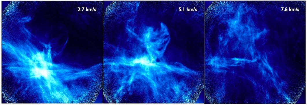
Figure 10: The COrE data will allow us to map the turbulent component of the Galactic magnetic field, and thereby characterize its role in shaping the diffuse interstellar medium and regulating star formation. The interstellar medium filamentary structure is illustrated here using HI spectroscopic observations obtained with the Dominion Radio Astrophysical Observatory. The three images correspond to three different velocity channels of one $4^{\circ}\times 4^{\circ}$ field (data from the Planck Deep Field HI survey, PI Peter Martin).

2.5.3 Galactic center

Nonthermal emission in the galactic center

The center of the Milky Way is the locus of high energy processes and a source of high energy cosmic rays which interact with the Galactic magnetic field as well as with interstellar matter. The polarization measurements of the plasma produced and diffusing from the Galactic Center (GC) region can set crucial constraints on the nature of the non-thermal emission from the GC region, on the large-scale structure of the magnetic field stretched along the outflowing regions (thought to have an intensity $\sim 50-500$ $\mu$G), on cosmic ray sources (likely SNRs), on the properties of the diffusive transport (and its effective time scale in comparison to advective time scales), and on the relative importance of hadronic and leptonic processes for the production and acceleration of nonthermal particles in the GC region.

Evidence for Dark Matter annihilation

Annihilation of Dark Matter (DM) particles ( $\chi$) followed by diffusion of secondary particles in the magnetic field of the GC region could be producing detectable $\gamma$-ray emission (due to $\chi\chi\to\pi^{0}\to\gamma+\gamma$) together with a diffuse halo (haze) of synchrotron and inverse Compton scattering of CMB (and other background) photons by energetic electrons (due to $\chi\chi\to X+\pi^{\pm}\to X+e^{\pm}$). The intensity, spatial extension, and spectrum of such emission depend on the details of the DM particle composition and annihilation cross-sections as well as on the Galactic magnetic field establishing the diffusion properties of the secondary particles produced in DM annihilation ([156]).

The existence of an anomalous microwave “haze” (in the WMAP data) coinciding with gamma-ray bubbles (in the Fermi-LAT data) centered around the GC has been largely debated and remains a controversial issue ([215, 160]. Emission from DM secondary particles was originally invoked to explain the anomalous WMAP microwave “haze”. This interpretation is at variance with an astrophysical scenario, where the putative haze would be associated with star formation in the GC region producing a fast wind with substantial quantities of cosmic ray ions that diffuse out to large angular scales on the sky [157].

The broad frequency and high sensitivity polarization survey of the GC region obtainable with COrE will provide an unprecedented view of the GC region and may lead to the discovery of a microwave “haze” associated with DM annihilation. Polarization is likely to play a key role in discriminating among competing possible interpretations. While strong polarization features (both in synchrotron and in inverse Compton emission) are expected in a scenario of SNe-driven outflows and winds, a DM-produced microwave “haze” is expected to have low polarization, because the secondary electrons are produced in situ along the DM density profile of the Galaxy, and are subject to a smooth and rather isotropic spatial diffusion in the GC magnetic field.

2.5.4 COrE sensitivity to polarized synchrotron

Accurate measurements of the polarized synchrotron radiation provide a unique probe to understand the structure of the Galactic magnetic field and to study the energy distribution of cosmic rays. The WMAP mission has provided first full-sky sensitive measurements of synchrotron-dominated sky emission polarization in the 20-90 GHz frequency range [177], providing also an estimate of the level of contamination by polarized galactic emission outside of the galactic plane, in regions useful for CMB studies.

The observing power of the low frequency channels of COrE will be ideal to extract the rich information encoded in the Galactic diffuse synchrotron component. Synchrotron radiation is intrinsically highly polarized, up to 70-75% in a completely regular field. The observed synchrotron polarization depends on the uniformity of the field orientation within the resolution element. The typical synchrotron sky temperature at 45 GHz—the lowest-frequency COrE channel—is $\sim 35\mu$K at intermediate Galactic latitudes. Assuming a polarization fraction of $\sim 60\%$, we predict the typical polarized signals to be of order $\sim 20\mu$K, with values depending on the features observed. Significantly higher values may be found in the loops and spurs, remnants of old supernova events close to the Galactic plane. At high latitudes, away from such local features, the expected degree of polarization should be only a few percent, resulting in polarized signals of a few $\mu$K. At intermediate latitudes, the polarization will lie somewhere between these two extremes.

The design sensitivity of the COrE 45, 75, and 105 GHz channels is approximately 0.4$\mu$K per resolution element (with beam-widths of 23^′, 14^′ and 10^′), corresponding to signal-to-noise ratios (SNRs) for synchrotron polarized emission of $\sim 50,$ $\sim 15$, and $\sim 4$, respectively. This will represent an enormous step forward compared to the 30 months of Planck data, which is expected to achieve SNRs for synchrotron polarimetry of $\sim 2$, $\sim 0.3,$ and $\sim 0.2$ at 44, 70, and 100 GHz, respectively, at similar angular resolution. The polarization maps from the Planck LFI 30 GHz channel and from the WMAP 23 GHz channel, both with high SNR ($\sim 10$) for polarized synchrotron, will constitute useful low-frequency ancillary data for the COrE analysis, in particular for disentangling synchrotron radiation from the contribution of the polarized component of interstellar dust.The exquisite polarization sensitivity of COrE will therefore deliver a high definition extraction of the synchrotron component in a Faraday-rotation free frequency domain.

2.5.5 Statistical analysis of Galactic magnetic fields with COrE

The accuracy of COrE polarization information on Galactic magnetic fields will provide a unique opportunity to study magneto-hydrodynamical turbulence and dynamo action in great detail within our Galaxy. It would greatly improve the reliability of any polarization data on small angular scales of the Milky Way in synchrotron light and thereby increase the spectral range of accurately probed magneto-hydrodynamical modes. Therefore the detection potential for relevant plasma physical processes and the characteristic scales of turbulent energy injection and dissipation would be increased considerably. Furthermore, accurate Galactic polarization data will be of eminent value for upcoming Faraday tomography measurements with telescopes like LOFAR, eVLA, ASKAP, and especially the SKA, which has a comparable timeline as COrE.

2.5.6 Faraday rotation free polarization

The COrE 45 or 60 GHz channels will provide a very accurate, highly resolved and detailed view on the synchrotron emission of our own galaxy. The polarization data permits to study the morphology of Galactic magnetic fields on global and local scales. CMB experiments measure at high frequencies and reveal there the original polarization structure, which do not suffer from Faraday rotation. Planck is currently increasing the angular resolution of such maps to a level comparable to ground based radio telescopes and COrE will boost the sensitivity and spectral information.

All ground-based radio-band synchrotron measurements of Galactic magnetic fields to date were carried out at much lower frequencies. Therefore they exhibit a high level of Faraday rotation and depolarization within the Galactic plane, hampering a direct analysis. COrE, by contrast, will unveil the polarization structure with essential no Faraday rotation (see Fig. 11). This data will make possible disentangling depolarization phenomena arising from Faraday rotation by the Galactic magnetic field and the superposition of contributions with different polarization orientations along the line of sight within the beam. Having this unrotated polarization information with high precision will be of importance for at least two scientific research directions:

• Accurately measured fluctuations in the synchrotron flux in intensity and polarization provide insight into magnetic turbulence. Several characteristic statistical properties are encoded in this data, for example the energy and helicity spectra as well as the spectrum of the magnetic tension force.

• Such data will allow Faraday rotation tomography measurements of our galaxy, which will be pursued with upcoming instruments like LOFAR, eVLA, ASKAP, and especially the SKA. Faraday tomography data can be expected to reveal further statistical information on Galactic fields, with very promising potential for detecting signatures of magneto-hydrodynamical processes.

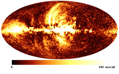
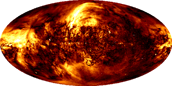
Figure 11: The WMAP 22.8 GHz all-sky polarized intensity map (upper panel) and the 1.4 GHz all-sky polarized intensity map (lower panel). The polarized intensities are shown greyscale coded from 0 to 100 $\mu$K for 22.8 GHz and from 0 to 570 mK for 1.4 GHz. Galactic Faraday-depolarization structures are visible in the lower frequency map. Data from [185, 177, 183] and figures from [182].

2.5.7 Magnetic spectra

The statistical properties of Galactic magnetic fields imprint themselves on observables such as the synchrotron intensity, polarization, and Faraday rotation measure. Methods to extract this information from observational data already exist and are being improved. Quantities highly relevant for an understanding of Galactic turbulence and dynamo processes are encoded in polarimetric data. Examples include:

• The magnetic energy spectrum, which is imprinted on intensity, polarization spectra and cross spectra [180, 181, 172, 173].

• The magnetic helicity spectrum, which can be measured from polarimetric data in combination with extragalactic Faraday data [175, 176]. Magnetic helicity is a key quantity to understand the inner workings of large-scale Galactic dynamos [168, 178, 179].

• The magnetic tension force spectrum, which is encoded in polarimetry data alone, and is powerful in discriminating between different magneto-hydrodynamical scenarios [184].

More physical relevant information might be encoded in the data. The above examples are only the quantities that are known today, for which a reconstruction from COrE data should be possible.

Due to our location within the galaxy, the angular fluctuations in observables correspond to physical magnetic field structures of different sizes. Disentangling these fluctuations in order to separate different physical scales such as the turbulent injection scale (see e.g. [174]) or dissipative scales will be challenging. Highly accurate polarimetric data, with full-sky coverage and precise calibration will be invaluable for this endeavor. The probing of a large range of physical scales simultaneously with high angular resolution makes it possible to monitor diagnostics of Galactic turbulence and dynamo theory.

Statistical analysis of the polarized diffuse synchrotron emission from WMAP and from radio surveys disagree. WMAP finds similar E-mode and B-mode angular power spectra while those obtained from radio surveys differ significantly [186]. Only more accurate measurements free from potential systematic effects can resolve this discrepancy. COrE will provide the necessary data and test the proposed theoretical models [187] at different angular scales to understand if the origin of this observational disagreement is explained by residual systematics, data analysis errors, or results from subtle astrophysical mechanisms.

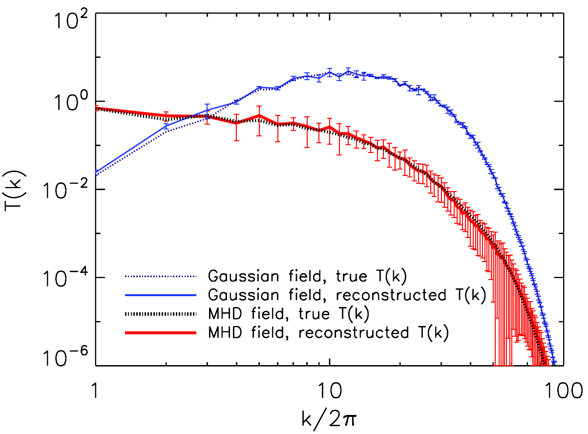
Figure 12: Tension force spectrum reconstructed from mock polarimetry data using the method of Stokes correlators (from [184]). The Gaussian random field was constructed to exhibit the same magnetic energy spectrum as the magneto-hydrodynamical simulation, but it has a different fourth-order statistic as measured by the Stokes correlators.

2.5.8 Faraday tomography

Faraday tomography provides three-dimensional information on magnetic fields and thereby restores some of the information lost in the line-of-sight projection of most astronomical observations. The depth information of a synchrotron emitter is encoded in the rate of rotation of its polarization angle as a function of wavelength $\lambda$. For different sources at different physical depth, and therefore different Faraday depth, this rate differs. Mathematically, the observed polarization as a function of wavelength squared is the Fourier transformed polarized emission per Faraday depth [171].

An inverse Fourier transformation can therefore reveal the polarization per unit Faraday depth [169]. This technique has already been successfully applied to radio data [170] and is extremely promising for upcoming radio telescopes. However the problem for many of these measurements, especially for long wavelength telescopes like LOFAR, is that the full $\lambda^{2}$-space can not be examined. In particular, the negative part of this space cannot be probed by any instrument. However information in the full $\lambda^{2}$-space would be required for a direct inversion of the Fourier relation. Therefore inverse methods have to be applied which benefit from any available information, in particular close to the unaccessible negative $\lambda^{2}$ range. Thus the information close to $\lambda=0$ as will be provided by the COre low frequency channels will be of greatest importance for Faraday tomography.

Since the Faraday tomographic data will provide much deeper insight into the details of Galactic magnetism than the two dimensional information discussed above, it is obvious that the scientific return will be even larger. Accurate all-sky COrE data will be crucial for the succuess of this technique for exploring the richness of magnetic phenomena in the Galaxy.

2.6 Extragalactic science

2.6.1 The Sunyaev Zel’dovich effect in galaxy clusters

The Sunyaev-Zel’dovich effect (SZE) [126] in which CMB photons suffer spectral distortion, or Comptonization, as a result of scattering off (thermal and nonthermal) electrons of the cluster atmosphere provides a powerful probe of the energetics, spectra, and stratification of the electron distribution in clusters [122, 123] due to its sensitivity to the details of the electron distribution of the cluster atmosphere. When scattered off hot electrons by Thomson scattering, CMB photons are boosted blueward in energy while the total number density remains constant. This effect leads to a distortion relative to the CMB blackbody spectrum, which is seen in the direction of a galaxy cluster according to the relation

$$\Delta I(x)=2\frac{(k_{\rm B}T_{CMB})^{3}}{(hc)^{2}}yg(x)$$ (14)

where $\Delta I(x)=I(x)-I_{0}(x)$, $I(x)$ is the observed spectrum in the direction of the cluster, and $I_{0}(x)$ is the unscattered CMB spectrum in the direction of a sky area contiguous to the cluster. Here $x\equiv h\nu/k_{\rm B}T_{CMB}$ is the re-scaled frequency where $h$ is the Planck constant and $T_{CMB}=2.726$ K the CMB temperature. The Comptonization parameter $y$ is given by the line-of-sight integral

$$y=\frac{\sigma_{T}}{m_{\rm e}c^{2}}\int P_{\rm e}d\ell~{}$$ (15)

in terms of the pressure $P_{\rm e}$ contributed by the electron population. $\sigma_{T}$ is the Thomson cross section, $m_{e}$ the electron mass, and $c$ the speed of light. The spectral shape of the SZE distortion $g(x)$ is given by

$$g(x)=\frac{m_{\rm e}c^{2}}{\langle\varepsilon_{\rm e}\rangle}\left\{\frac{1}{\tau_{e}}\left[\int_{-\infty}^{+\infty}i_{0}(xe^{-s})P(s)ds-i_{0}(x)\right]\right\}$$ (16)

in terms of the photon redistribution function $P(s)$ and

$$i_{0}(x)=I_{0}(x)/[2(k_{\rm B}T_{CMB})^{3}/(hc)^{2}]=x^{3}/(e^{x}-1)\;.$$ (17)

The quantity

$$\langle\varepsilon_{\rm e}\rangle\equiv\frac{\sigma_{\rm T}}{\tau_{e}}\int P_{e}d\ell=\int_{0}^{\infty}dpf_{\rm e}(p)\frac{1}{3}pv(p)m_{\rm e}c\;,$$ (18)

where $f_{e}(p)$ is the normalized electron momentum distribution function, is the average energy of the electron plasma [120]. The optical depth of the electron population along the line of sight $\ell$ is

$$\tau_{\rm e}=\sigma_{T}\int d\ell~{}n_{\rm e}\;.$$ (19)

The photon redistribution function $P(s)$, where $s=\ln(\nu^{\prime}/\nu)$ is the logarithm of the CMB photon frequency change $\nu^{\prime}/\nu$, can be calculated by repeated convolution of the single-scattering redistribution function, $P_{1}(s)=\int dp~{}f_{\rm e}(p)~{}P_{\rm s}(s;p)$, where $P_{s}(s;p)$ expresses the physics of inverse Compton scattering. The previous description is general enough to be applied to both thermal and nonthermal plasmas as well as to a combination of the two (see [120, 119] for details).

A velocity (or kinematic) SZE also arises if the scattering medium causing the thermal (or non-thermal) SZE is moving relative to the Hubble flow. In the reference frame of the scattering gas the CMB radiation appears anisotropic, and the effect of the inverse-Compton scattering is to re-isotropize the radiation slightly. Back in the rest frame of the observer the radiation field is no longer isotropic, but shows a structure towards the scattering atmosphere with amplitude proportional to $\tau_{e}V_{z}/c$, where $V_{z}$ is the component of peculiar velocity of the scattering atmosphere along the line of sight [201, 202, 203]. The intensity change due to the kSZE is given by

$${\Delta I\over I}=-\tau_{e}\beta_{z}h(x)$$ (20)

with $\beta_{z}\equiv{V_{z}\over c}$ and $h(x)={xe^{x}/e^{x}-1}$ in the nonrelativistic regime [114]. A relativistic generalized derivation of the kSZE has been given in the framework of the general Boltzmann equation and in the covariant formalism [204].

Direct numerical integration of the Boltzmann collision term have been done in this context [210] that confirm the validity of analytic formula for the description of kSZE (see, e.g., [211, 212, 213, 214]) the Rayleigh-Jeans limit.

Due to its redshift-independent nature, the SZE is also a powerful cosmological probe [114, 197, 196, 200]. and can check for potential traces of cluster evolution better than other cosmological probes [199, 195], in particular for galaxy clusters in the medium mass regime. The SZE can be used to determine accurately the main parameters of a $\lambda$CDM cosmology and the dark energy equation of state [115], and also to set constraints on modified gravity scenarios [116] and on the properties of primordial magnetic fields [117]. To realize this program the SZE in galaxy clusters must be determined with very good accuracy in order to derive accurate and unbiased cosmological probes.

In this context, precise observations of the SZE at microwave and millimeter wavelengths are crucial for unveiling the detailed structure of cluster atmospheres, their temperature distribution, and the possible presence of suprathermal or nonthermal plasma because the high-frequency part (i.e., $\nu\lower 2.15277pt\hbox{$\;\buildrel>\over{\sim}\;$}350$ GHz) of the SZE spectrum is more sensitive to the relativistic effects of the momentum distribution of the electrons plasma [120, 122, 119]. This is even more so for galaxy clusters with a complex plasma distribution as found in powerful merging clusters such as the exemplary case of the Bullet cluster (1ES0657-56) [198] (see Fig. 13).

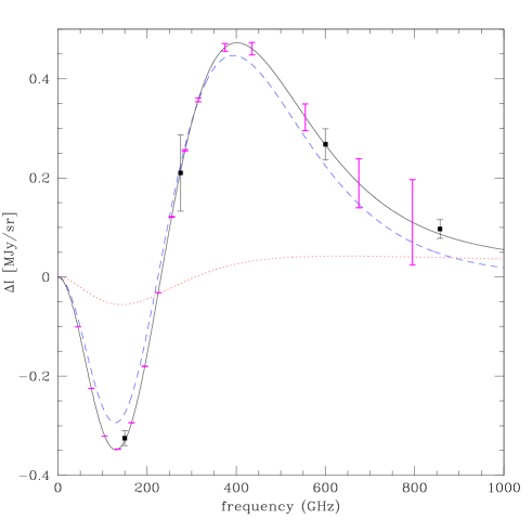
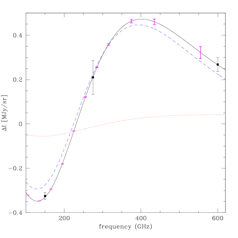
Figure 13: Left: The SZE spectrum at the Bullet cluster center modelled with a thermal plus nonthermal plasma. Shown are: thermal plasma with $kT=13.9$ keV, $\tau=1.1\times 10^{-2}$ (blue dashed); nonthermal plasma with $p_{1}=1$, $s=2.7$ and $\tau=2.3\times 10^{-4}$ (red dotted); total SZE produced by the sum of the two plasmas (black solid). The observed data are shown as black squares plus uncertainties and the COrE sensitivity at the various frequencies are shown by magenta error bars. Right: Same as in the left panel but zoomed in the region where the SZ effect spectrum of the Bullet cluster is sensitive to the relativistic effects and the COrE sensitivity is highest.

Polarization $\Pi$ of the SZE arises from various dynamical and plasma effects related to plasma transverse velocities and multiple scattering processes. These effects include galaxy cluster transverse motion ($\Pi_{k}\propto\beta^{2}_{t}\tau$ in the Rayleigh-Jeans (RJ) regime with $\beta_{t}=V_{t}/c$), transverse motions of plasma within the cluster ($\Pi_{v}\propto\beta_{t}\tau^{2}$ in the RJ regime), multiple scattering between electrons and CMB photons within the cluster ($\Pi_{th}\propto\Theta\tau^{2}$ in the RJ regime, with $\Theta=kT_{e}/m_{e}c^{2}$) [127, 118, 125]. The general covariant relativistic derivation of the SZE polarization for both thermal and nonthermal plasma [125] generalizes the nonrelativistic derivation [127] taking into account the direct dependence of the SZE polarization spectra on the properties of the electron distribution in the atmospheres of galaxy clusters and other cosmic structures. We stress that the SZE polarization signals in clusters have spectra quite different from the intensity SZE spectra (see Fig. 14).

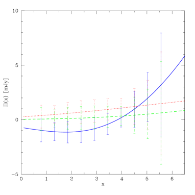
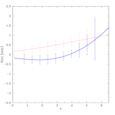
Figure 14: Left. The spectral shape of the maximum SZE polarization signal for a cluster with $kT=15$ keV and $\tau=5\cdot 10^{-2}$ are compared to the COrE polarization sensitivity (shown as error bars) at the various frequencies: thermal SZE polarization due to double scattering $\Pi-{th}\propto(kT_{e}/m_{e}c^{2})\tau^{2}$ (blue curve and COrE error bars), polarization due to tranverse motion of gas inside the cluster $\Pi_{v}\propto\beta_{t}\tau^{2}$ (green curve and COrE error bars), polarization due to transverse bulk motion of the cluster $\Pi_{k}\propto\beta_{t}^{2}\tau$ (red curve and COrE error bars). A cluster size of 3 arcmin radius has been considered. Right. The thermal SZE polarization spectrum (blue solid) from a stacking analysis of 20 clusters with $kT>10$ keV and $\tau>0.03$ is compared with the same analysis for the kinematic SZE polarization spectrum (red dotted). The statistical uncertainties refer to a stacking analysis produced with COrE.

Combining intensity and polarization observations of the SZE with the frequency dependence and spatial distribution of the Stokes parameters of the SZE can uncover unique details of the 3d (projected and along the line of sight) velocity structure of the intracluster plasma, of its 3d pressure structure and of the influence of a structured magnetic field in the stratification of the intracluster plasma, and therefore provides a full 3d tomography of the structure of cluster atmospheres. Analogously, the combination of the intensity and polarization observations of the kinematic SZE (and its frequency dependence) can yield crucial information on the 3d distribution of the cosmological velocity field traced by galaxy clusters. Specifically, the ratio $\delta I/\Pi_{th}$ yields direct information on the plasma optical depth $\tau$, and the ratio $\delta I/\Pi-{v}$ on the combination $\tau\cdot\beta_{t}$, thus allowing to use intensity and polarization SZE measurements to fully disentangle the pressure and velocity structure of the cluster atmospheres.

Recent observational results and theoretical analyses have clearly shown that an effective study of the SZE (both in intensity and polarization) should be carried out over a wide frequency range including especially high frequencies where the effects of the electron distribution function are larger and allow millimeter observations to be used to derive the fundamental parameters of the cluster atmosphere and its plasma stratification and dynamics.

SZE observations in the millimeter range are becoming available with PLANCK-HFI (in the $\sim 100-850$ GHz range) and HERSCHEL-Spire (in the $\sim 600-1200$ GHz range). HERSCHEL, however, lacks spectral coverage in the low-$\nu$ part of the SZE spectrum that is important for an unbiased determination of the main cluster parameters (i.e., the gas density, temperature, and cluster peculiar velocity), while PLANCK-HFI suffers from a limited sensitivity and spatial resolution needed to determine and resolve the cluster parameters for the majority of medium- and small-mass systems. At best very limited information on the SZE polarization can be obtained with these instruments. Other experiments from the ground (e.g. SPT and ACT) are producing large area surveys of cluster with SZE measurements in the low-$\nu$ part of the spectrum (i.e. at $\nu\approx 150$ Ghz) but cannot provide an all-sky SZE, do not have access to the high-$\nu$ part of the SZE spectrum (which is crucial to obtain physical information on the structure of cluster atmospheres) and strongly suffer (as in any ground experiment) from atmospheric opacity and frequency band inter-calibration effects.

The wide frequency coverage (from 45 to $\sim$ 800 GHz) and the unprecedented sensitivity in both intensity and polarization of COrE will provide a substantial improvement in the study of the SZE in galaxy clusters and in other cosmic environments.

• COrE will detect more than $\sim 5\cdot 10^{4}$ clusters at 135–165 GHz and $\sim 3\cdot 10^{3}$ clusters at 375 GHz with thermal SZE above the sensitivity threshold, assuming that PLANCK will detect $\approx 10^{3}$ clusters in the HFI 143 GHz channel. These clusters will also be resolved better owing to the improved spatial resolution of COrE (i.e., $\sim 6.4$ arcmin at 165 GHz and $\sim 2.8$ arcmin at 375 GHz) compared to the $\sim 7$ and $\sim 5$ arcmin resolution of Planck at similar frequencies.

• CorE will provide full coverage of the SZE spectrum with a sensitivity that allows a systematic study of the thermal, multi-temperature, and nonthermal properties of many galaxy clusters (see Fig. 13). Such studies will be possible for several hundreds of galaxy clusters with $kT\lower 2.15277pt\hbox{$\;\buildrel>\over{\sim}\;$}2-3$ keV.

• COrE will provide a spatially resolved spectral study of many nearby clusters, especially at high $\nu$ where relativistic effects of single- and multi-temperature, or supra-thermal, plasmas are relevant. In about 100 clusters with angular size larger than $\sim 5$ arcmin radius, COrE will also be able to perform spatially resolved spectral studies of the SZE in the frequency range $\sim 200-600$ Ghz.

• COrE will provide relevant constraints on the polarization of the thermal SZE in many nearby, hot clusters. Fig. 14 shows that even clusters with high temperatures $kT\approx 15$ keV and high optical depth $\tau\approx 5\cdot 10^{-2}$ produce maximum SZE polarization signals that are marginally detectable by COrE in single cluster observations. However a stacking analysis of even small samples ($\sim 20$) of hot and dense galaxy clusters observed with COrE at several frequencies would allow one to determine statistically up to $\sim 200$ GHz the polarization signals of the thermal SZE for clusters with $kT>10$ keV and $\tau>0.03$ (see Fig. 14). A sample of powerful merging clusters would set limits on the polarization features due to transverse gas velocities $V_{t}\lower 2.15277pt\hbox{$\;\buildrel>\over{\sim}\;$}500$ km/s. Finally a relatively large sample ($\sim 10^{2}$) of clusters could be used to set limits on the three-dimensional velocity field by observing the kinetic SZE polarization.

• COrE will provide a more detailed description of the millimeter band point-like source contamination to determine the spectral and spatial properties of the cluster SZE (and of its polarization) especially in the frequency range probed by COrE.

• COrE will provide both detailed observations and unprecedented constraints on the SZE expected in other astrophysical plasmas such as the lobes of radio galaxies and the plasma halos of galaxies [123]. In fact, as a consequence of the pervading presence of inverse Compton scattering of CMB photons in extended radio galaxy lobes, a SZE from the lobes of radio galaxies is inevitably expected (as first proposed and discussed by [124]). This nonthermal, relativistic SZE has a particular spectral shape that depends on the shape and on the energy extent of the spectrum of the electrons residing in the RG lobes (see [124, 198]). The SZE in RG lobes has not yet been detected. Only loose upper limits have so far been derived on the SZE from these sources (see [114]; see also [129] for a recent attempt to detect this effect at radio wavelengths). The wide spectral range of COrE and its enhanced sensitivity (also in polarization) will endow this experiment with the unique ability to detect the nonthermal SZE in a sample of more than 10 giant radio galaxies.

2.6.2 Non-polarized point sources

In total intensity COrE will be so sensitive that it will reach the source confusion limit. We can use galaxy counts from large area Herschel surveys (H-ATLAS and HerMES, Clements et al. 2010; Oliver et al. 2010) [131, 146] at COrE wavelengths to determine the confusion limits for the COrE beamsize and thus the number of sources that will be detected over the sky. For a beam FWHM of $1.3^{\prime}$ at 795 GHz and of $1.9^{\prime}$ at 555 GHz, we find $5\sigma$ detection limits of $\simeq 96\,$mJy and of $89\,$mJy respectively, if we take into account only the Poisson fluctuations. If we allow for the effect of clustering (Negrello et al. 2007) [144], the $5\sigma$ confusion limits increase to 119 mJy and to 127 mJy at 795 and 555 GHz, respectively.

Surveys of small areas of the sky are already available at 350$\mu$m (857 GHz) with somewhat better angular resolution and depth from Herschel. In Fig. 15 we show the $4^{\circ}\times 4^{\circ}$ region surveyed by H-ATLAS (Eales et al. 2010; Rigby et al. 2010) [136, 148] smoothed to the 1.3 arcmin FHWM beam of COrE  at 795 GHz. Among the brightest objects in this H-ATLAS image are five strongly lensed background galaxies lying at $z\sim 2$–3, which can easily be identified by their red far-IR color and absence from radio surveys (Negrello et al. 2010). [145]. COrE will be able to use its highest frequency channels to provide a similar selection of high redshift lensed far-IR sources, but this will be possible beyond the limited areas covered with Herschel.

Using an updated version of the Negrello et al. (2004) model [144], we estimate that COrE will be able to detect at 795 GHz approximately $1.3\times 10^{4}$ strongly lensed high-$z$ dusty galaxies above $|b|\sim 20^{\circ}$, where Galactic confusion should be of relatively minor importance. In addition, it will detect, at the same frequency, $\simeq 4\times 10^{4}$ normal and starburst galaxies and $\simeq 540$ unlensed high-$z$ proto-spheroidal galaxies. Interestingly, the strongly negative K-correction that makes (sub-)mm surveys extraordinarily well suited for detecting high-redshift star-forming galaxies, shifts their expected distribution to higher redshifts at longer wavelengths. We thus expect that millimeter surveys with COrE will lead to the detection of ultra-bright strongly lensed galaxies at very high redshifts.

Furthermore, COrE will detect, at $|b|>20^{\circ}$, some 1500 blazars in the poorly explored sub-millimeter range, close to the synchrotron peak of the most luminous objects of this class.

Figure 15: H-ATLAS 350$\mu$m SDP field ($14.4\,\hbox{deg}^{2}$) smoothed to COrE resolution. The brightest sources in this image include an unusual clump of Galactic dust emission, possibly a high Galactic latitude Bok globule, a WMAP blazar (Gonzalez-Nuevo et al. 2010) and five strongly lensed high redshift ($z\sim 2$–3) dusty galaxies (Negrello et al., 2010), all potentially detectable by COrE. COrE  will select such extremely interesting sources over most of the whole sky.

2.6.3 Characterizing extragalactic sources

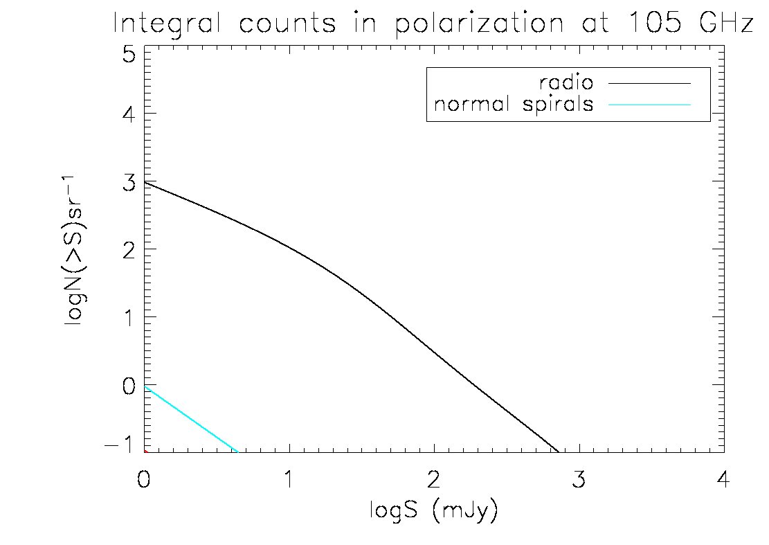
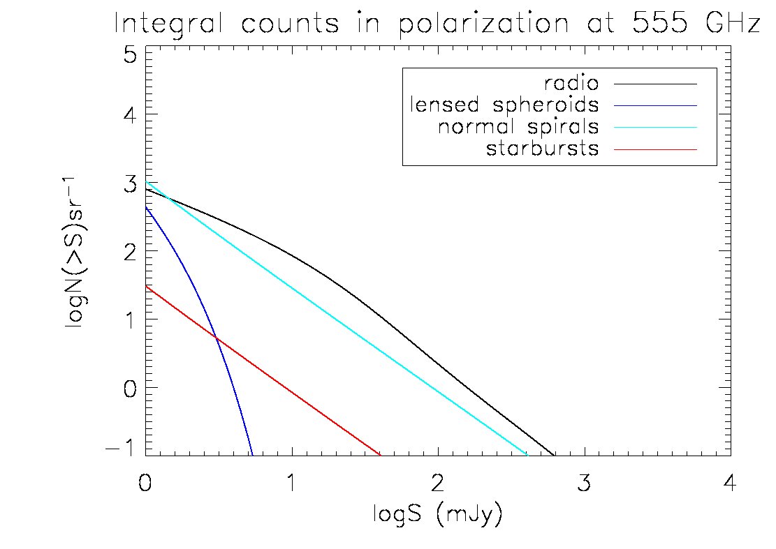
Figure 16: Expected integral counts as a function of the polarized flux of radio sources and of different populations of dusty star-forming galaxies at 105 and 555 GHz.

Measurements of the polarization properties of radio sources at millimeter and sub-millimeter wavelengths provide important insights into the physical properties (and in particular into the structure of magnetic fields) of the innermost compact regions of relativistic jets in AGNs. These measurements will be also essential to assess the point sources contamination of CMB polarization maps. In fact, at high Galactic latitudes, radio sources are expected to be the main contaminant on scales $\raise 1.29167pt\hbox{$<$\kern-7.5pt\raise-4.73611pt\hbox{$\sim$}}0.5^{\circ}$ up to frequencies of a few hundred GHz (De Zotti et al. 1999; Tucci et al. 2004, 2005). [216, 151, 271].

The only blind polarization surveys presently available are those produced by WMAP (Wright et al. 2009). [153]. López-Caniego et al. (2009) [141] reported the detection in polarization, in at least one WMAP channel; however, of 22 objects five are doubtful. PLANCK can double the number of detections, but the sample will still be too limited for a meaningful study of polarization properties of the several radio source populations.

Ground based studies of high-frequency polarization properties of radio sources have been carried out by following-up samples drawn from surveys in total intensity. In spite of recent efforts (Jackson et al. 2010; Agudo et al. 2010) [139, 130], polarimetric data at millimeter wavelengths are limited, and essentially non-existent at sub-millimeter wavelengths.

The most extensive polarization information on complete samples selected at high radio frequencies was obtained at $\simeq 20\,$GHz (Ricci et al. 2004; Massardi et al. 2008; Jackson et al. 2010) [147, 142, 139]. Radio sources are found to be significantly polarized (up to $\raise 1.29167pt\hbox{$>$\kern-7.5pt\raise-4.73611pt\hbox{$\sim$}}30\%$, Shi et al. 2010, [217] although the median polarization degree is approximately 3%).

Polarized emission in giant radio galaxies is an exceptionally powerful tool to understand the origin of relativistic particles, ultra-high-E cosmic rays, and magnetic fields (see, e.g., Kronberg 1994) [140]). In regions of the RG lobes where shocks are strongest, the inflation of the lobe is likely accelerating particles to very high energies, producing also quite flatter synchrotron spectra (see e.g. [133]), and relatively high degrees of polarization (20-40%) that could be observed with COrE in many nearby objects. In addition, Inverse Compton scattering of CMB photons in giant radiogalaxy lobes produces an SZ effect (Colafrancesco 2008) [132], whose spectrum (both in intensity and polarization at a level of 10-20%) is best observed at high frequencies where it shows a maximum and a flat spectrum in the range 500-1000 GHz that could be observed with COrE in a dozen of nearby extended objects. The combination of polarized synchrotron and SZ effect in giant radio lobes offers the unique opportunity to disentangle efficiently the distribution of the relativistic electrons from that of the magnetic field and to provide, for the first time, a complete 3d tomography of the atmospheres of these cosmic structures.

Very little is known about the polarization of dusty galaxies that dominate the counts in total intensity above $\simeq 100$–200 GHz, but there are indications that it is probably $\leq 1\%\,$ (Seiffert et al. 2007; Greaves & Holland 2002) [138, 149], as expected because of the complex structure of the magnetic field resulting in cancellations of polarization directions.

The spectacular sensitivity of COrE provide the first large sample of sources blindly selected in polarization. Because of the polarized flux is on average a small fraction of the total flux, source confusion is far less of a problem for polarization than for total intensity. Adopting an average polarization degree of 3% for radio sources and of 1% for dusty star-forming galaxies, and using the model by De Zotti et al. (2005) [134] for the former population and the model by Negrello et al. (2007) [144] for the latter, we find that the confusion noise is always sub-dominant and becomes negligible above 100 GHz, at least in high Galactic latitude regions where polarized diffuse emissions are low provided that the CMB can be efficiently removed.

As illustrated by Fig. 16, at 105 GHz we expect to detect the polarized flux of $\simeq 320$ radio sources per steradian above the $5\sigma$ detection limit $S_{\rm lim}=5(\sigma_{\rm noise}^{2}+\sigma_{\rm conf}^{2})^{1/2}\simeq 3\,$mJy. At higher frequencies the polarized dust emission from dusty star-forming galaxies should also be detectable. Under the above assumptions for the mean polarization degree, we have $\simeq 12$ radio sources and $\simeq 5$ normal spiral galaxies per sr with polarized flux larger than the $5\sigma$ detection limit of $\simeq 32.5\,$mJy at 555 GHz. At 795 GHz the $5\sigma$ detection limit is $\simeq 48.5\,$mJy and the expected numbers of detections per sr are of $\simeq 6$ radio sources and of $\simeq 16$ dusty galaxies.

3 Separation of the polarized microwave sky into components

The COrE mission is designed to achieve unprecedented sensitivity in fifteen frequency channels ranging between 40 and 800 GHz. COrE is designed to serve as a comprehensive explorer of all astrophysical emissions in this wavelength range. The sensitivity of the mission in each of these channels is designed to reach the many science goals discussed in Sect. 2. Achieving these science goals requires the capability to avoid astrophysical confusion—that is, the capability to separate the emissions from different astrophysical sources. For a recent overview of diffuse component separation methods see [236]. A comparison of existing methods in preparation for the PLANCK mission can be found in [252].

In the tour of the microwave sky in the bands covered by COrE, we described how the observed emission in a particular frequency channel is the linear superposition of several components arising from distinct physical processes. The various diffuse components identified—mainly emissions from the galactic ISM and the primordial CMB—have differing frequency dependences. This feature allows their separation, which is a prerequisite for all the science described in the preceding sections.

Since the COBE detection, the development and application of component separation methods have been a very active area of CMB research, and many methods have been successfully applied to temperature component separation, both on real data and on simulations for validation. In fact, until now foregrounds have been much feared but have turned out to be less of a problem than anticipated, at least for the measurement of the temperature power spectrum. In practice, many methods have been developed and optimized. At their core, these methods derive from a number of simple ideas, including:

• Masking the brightest point sources and modelling the residuals;

• Cutting out the galaxy, less so for small wavenumbers and more aggressively for larger wavenumbers;

• Extrapolating the frequency dependence of foreground components using physically motivated emission laws, or empirical frequency scaling obtained from correlation studies;

• Using ‘blind’ methods to let the data express its natural decomposition into components through the hypothesis of statistical independence.

For polarization studies, a much higher degree of cleaning through component separation is required because for the B modes the polarized foregrounds outshine the targeted signal in all frequency bands by about two orders of magnitude or more (see Fig. 17).

Below we review in more detail existing work, discussing its relevance to the component separation for COrE, and justify the rationale for the COrE frequency bands. We also demonstrate that the expected final performance for measuring the CMB B modes in the presence of polarized foregrounds matches the requirements of the mission.

3.1 Sky emission modelling and component separation methods

Over almost all the sky except very near the Galactic plane, astrophysical emissions in the millimeter wavelength range originate from sources which are optically thin. The total observed emission is consequently simply the sum of all emissions along the line of sight, without obscuration of one source by another. At each frequency $\nu$, the total observed emission in direction $p$ is then, for $N$ distinct components:

$$x(\nu,p)=\sum_{i}^{N}x_{i}(\nu,p)$$ (21)

where $x_{i}(\nu,p)$ denotes the emission from the component $i$.

3.1.1 Linear mixtures

The coherence of the astrophysical emissions across frequencies is what allows for the identification and separation of the contributions of the individual components. In an idealized case, each component is modelled with a single template $s_{i}(p)$ scaling with frequency according to a single emission law $a_{i}(\nu)$. We then have

$$x(\nu,p)=\sum_{i}^{N}a_{i}(\nu)s_{i}(p).$$ (22)

If the frequency dependence $a_{i}(\nu)$ is known (from physical principles) for all components, then separating the different contributions amounts simply to inverting the linear system to measure the intensity $s_{i}(p)$ of each emission in each pixel. Methods for doing so in the presence of instrumental noise and under various hypotheses about the number and statistical properties of the component emission maps have been discussed by numerous authors in the context of CMB temperature measurements [269, 245, 229, 233].

In practice, the frequency scaling for the astrophysical components is known only to limited precision, either because of imperfect calibration of the measurements (e.g., for the CMB component), or because of intrinsic uncertainty as to the parameters of the physical emission processes (e.g.i, for emission from the galactic ISM). In this case component separation for CMB applications can be achieved using Independent Component Analysis (ICA) methods [222, 264, 253, 234, 226]. Estimates $\widehat{s}_{i}(p)$ of the component emission templates $s_{i}(p)$ are obtained, for instance, as linear mixtures $\widehat{s}_{i}(p)=\sum_{j}w_{ij}x(\nu_{j},p)$, where the weights $w_{ij}$ maximize a given measure of independence between the reconstructed components $\widehat{s}_{i}(p)$. ICA methods can also be tuned to estimate directly the elements $A_{ij}=a_{i}(\nu_{j})$ of the “mixing matrix” $A$ and then to invert the system. In addition to $A$, some methods also estimate second-order statistics of the components [234, 255], which is of direct cosmological interest for the measurement of the CMB power spectrum and also allows using these estimates to reconstruct maps of the individual components by Wiener filtering.

However astrophysical foregrounds are not always independent. Galactic emissions are all concentrated in the galactic plane, which gives rise to correlations among the components. Moreover, the components are physically interdependent. Spinning dust emission arises from dust particles that also emit greybody radiation. For polarized emissions, the same magnetic field confines trajectories of electrons responsible for synchrotron emission and controls the alignment of dust grains emitting polarized radiation at submillimeter wavelengths. Hence the assumption of independence, which is the statistical foundation of the ICA methods, does not strictly hold. Methods exists which deal also with partially correlated foreground emissions [223, 227, 230].

Most of the methods developed for CMB temperature can be applied with minor modifications to separate polarization maps [265, 221, 218, 225].

3.1.2 More complex sky emission

In reality, the linear mixture model of eqn. 22 holds only approximately [270]. As a next level of complexity, the emission law $a_{i}(\nu)$ of many of the components is not strictly the same at different pixels. As observed by several authors [259, 231, 247, 242], synchrotron spectral indices between 408 MHz and few GHz vary from pixel to pixel. In addition, the steepening of the synchrotron emission law at high frequencies (above $\sim$30 GHz) due to the aging of cosmic rays is expected to be inhomogeneous on the sky. Similarly, the emission law of galactic dust depends on the local distribution of the dust grain properties (size, chemical composition, temperature, etc.). Finally, the sky emission comprises also integrated emission from a large population of extragalactic objects, each of which has its own emission law, red-shifted (for the farthest ones) by the cosmological expansion. In summary, astrophysical foreground emission is complex, and the linear mixture model is at best a crude approximation, which is totally inadequate for sensitive observations. For COrE, which targets a sensitivity 20 to 30 times better than the previous CMB space mission, the difference between real foregrounds and their approximation on the basis of a linear model is expected to be orders of magnitude larger than the sensitivity. Component separation must deal with this complexity. This impacts the design of the mission, which must provide the information needed to extract the very tiny B-mode signal from a sky emission dominated by poorly characterised foregrounds.

Two main approaches have been explored for the separation of such complex foregrounds. The first is based on multi-frequency linear filtering, and specifically targets CMB science. The second is based on a pixel dependent fit of all physical or phenomenological parameters describing the emission of all components, using as input data the observation of the sky in all the available frequency bands. Both approaches and variants are discussed below.

3.1.3 Linear filters

One of the most challenging component separation problems is the extraction of CMB polarization B modes down to a level $r\simeq 10^{-3}$ as targeted by COrE. Even at high galactic latitude, the power spectrum of CMB B modes is expected to be several orders of magnitude below galactic contamination [271, 240].

Even if ICA methods are not well suited to separate components for which the linear mixture model of eqn. 22 does not hold, component separation methods exist which exploit the independence of the CMB from other emissions, and address specifically the problem of separating this single component from a complex mixture of unidentified, and possibly correlated, foregrounds.

The SMICA method [234, 230], in particular, is a very powerful method to directly estimate either the tensor-to-scalar ratio $r$, or the power spectrum of CMB pseudoscalar modes $C_{\ell}^{BB}$, as well as the errors of the estimated CMB parameters in the presence of foregrounds. So far this approach, for polarzation, has been tested on simulations made with synchrotron and dust polarized foregrounds as simulated with version 1.6.4 of the PSM. The simulated synchrotron is modeled with pixel-varying amplitude and spectral index, and the simulated dust with two greybodies with varying amplitudes and temperatures. With the CMB included and point sources neglected, this makes a total of 7 different maps which model the total polarized emission.

Using these simulations, the work described in [225] shows that for various configurations of a space mission with high sensitivity, high angular resolution, and at least 8 frequency channels, the tensor to scalar ratio can be measured down to $r\simeq 10^{-3}$ with a signal-to-noise ratio of order 5. Moreover, these results are shown to be robust against minor changes of the simulated foregrounds (adding synchrotron curvature, some point source contamination, and increasing the level of polarized dust emission).

It should be noted that the simulated polarized sky uses 7 maps, and the successful instruments have at least 8 frequency channels. As discussed in [229], the impact of a varying emission law can be linearized to first order, so that the total sky emission (CMB and foregrounds) is, if modeled as a linear mixture of fixed templates, about 7-dimensional. In practice, however, the number of templates used to marginalize over foreground emission in [225] is only 4, which means that some of the complexity induced by varying spectral parameters have a negligible impact on the ability to measure the CMB. Loosely speaking, it also means that about 4 remaining channels (eight minus four) contribute to the sensitivity to the CMB.

As an alternate approach to SMICA, several authors have used the simple “internal linear combination” ILC method to investigate component separation for measuring CMB B-modes. Instead of fitting directly for the B-mode power spectrum, the ILC first builds a CMB map by forming a linear combination of the input observations that minimizes the total variance of the reconstructed map, up to the constraint that the response to the CMB should be unity. The power spectrum of the reconstructed CMB map is then computed, taking into account biases and additional variance induced by foreground and noise residuals in the reconstructed map.

Although less powerful than SMICA, ILC has the virtue of simplicity. It is however prone to subtle errors, for example biases resulting from correlation between CMB and foregrounds [244, 235]. Calibration errors can become amplified in a high signal-to-noise regime [237]. These biases, however, will be small (as compared to errors due to noise, cosmic variance and residual foregrounds) for measurement of B modes with COrE.

3.1.4 Parametric fitting

The parametric method directly fits a parametric model of the emission of all components in each pixel [241, 238, 268]. In current implementations, the method offers only moderate capability to disentangle low frequency foregrounds due to a lack of sensitive low frequency observations. Accuracy in the measurement of the parameters is limited by the instrument noise. The capability to constrain many parameters is limited by the insufficient number of measurements at different frequencies. For suborbital experiments less sensitive than COrE, observing clean regions of the sky, a frequency coverage limited as compared to that of COrE may be sufficient to reach $r\simeq 4\times 10^{-2}$ after polarised component separation with a parameter-fitting technique [266]. COrE is, however, targetting a sensitivity fourty times better than that on the tensor to scalar ratio, which requires significantly better foreground cleaning in these regions of low foreground contamination, but also a significantly larger sky area.

For accurate component separation with COrE, the emission law of the synchrotron should then be represented with 2 or 3 parameters (amplitude, spectral index, and running due to the aging of the relativistic electrons), CMB with 1 parameter (temperature), and thermal dust is usually fit with 3 to 6 parameters (amplitude, spectral index, and temperature for one or two greybodies). Free-free emission requires one or two parameters per pixel (amplitude and average electron temperature), and thermal SZ effect also one or two (amplitude and electron temperature). Spinning dust emission is predicted to have a smooth spectrum, limited to low frequencies below the frequency coverage of COrE. Molecular line emissions, in full generality, require one parameter per line, but impact only frequency bands containing strong molecular lines. The main polarized emissions being the CMB, synchrotron, and dust, an accurate fit for polarization requires measuring sky emission in at least 6-10 frequency bands. For temperature, about 5 additional bands are necessary.

3.2 The choice of frequency bands

Proper selection of frequency bands for the space mission is essential to successful component separation. For each pixel of the sky, it is important to have enough independent measurements to constrain all parameters of all the emission model. Given the level of rejection targeted, the bands must provide the capability of checking consistency internally. For polarized component separation, the frequency channnels more numerous than the number of linear components or model parameters.

Since 6-10 parameters are necessary to describe the polarized components (synchrotron, CMB and dust), at least as many frequency channels are required. Redundancy is achieved by providing several additional channels beyond this minimum.

For the intensity maps, the spectral coverage must also allow for fitting unpolarized emissions: free-free, spinning dust, thermal Sunyaev Zel’dovich effect, and molecular lines, with one or more parameter for each. Hence we require a conservative four to five additional frequency channels for adequate frequency coverage in temperature, for a total of ten to fifteen parameters to fit unpolarized emission. In order to measure as many parameters as required to fit and interpret the data, we design COrE to observe the sky in 15 different frequency bands. This is also useful to avoid using the CMB sensitive channels as polarized foreground tracers.

Broad spectral coverage is important not only for addressing the COrE science objectives, but alsoto test and guarantee a posteriori the effectiveness of component separation. This broad spectral coverage is a strength of the COrE design as compared to previously proposed or currently operating CMB polarization experiments.

3.3 Measuring $r$ in the presence of foreground emission

To study the COrE capabilities more specifically, several independent foreground removal simulations were carried out. We now describe the preparation of simulated data sets for this study and the methods developed to extract the CMB B mode signal. We first describe simulations performed for this analysis, and then results obtained with two methods: The first approach is an ILC in needlet space (NILC), very similar to what has been done in [235] for WMAP temperature maps. The second is based on a pixel-based linear component separation method (pix-LCS), for which errors due to noise and foreground residuals have been forecast for COrE with the method described in [228].

3.3.1 Simulations with the PLANCK Sky Model

The PLANCK Sky Model (PSM) is a data and software package developed in preparation for the PLANCK mission. It serves as a tool that predicts or simulates temperature and polarization emissions of the different astrophysical components relevant to sky observation in the 3 GHz–3 THz frequency range. The PSM implements models of the following emissions: primordial CMB, the galactic ISM (synchrotron, free-free, thermal dust, spinning dust, molecular CO lines), the thermal and kinetic Sunyaev-Zel’dovich effects, known radio and infrared sources, unresolved infrared galaxies (the CIB). Of these, CMB, synchrotron, thermal dust and emission by known point sources are polarized in the PSM version used for the present study (v1.7).

CMB emission is modeled as a multivariate ($T$, $E$, $B$) Gaussian random field, the statistics of which are fully described by power spectra $C_{\ell}^{TT}$, $C_{\ell}^{TE}$, $C_{\ell}^{EE}$, and $C_{\ell}^{BB}$, computed using the CAMB software for WMAP 7-year best-fit cosmological parameters. Tensor modes at the level of $r=10^{-3}$ or $r=5\times 10^{-3}$ have been added (see below). B modes from lensing shear are modelled as Gaussian for this application.

The polarized galactic emission used includes polarized synchrotron and polarized dust. A 23 GHz synchrotron template is obtained from the analysis of WMAP data described in [257]. The polarisation fraction ranges from 0 to 70 %, with an average over the sky of about 18%. Two 100 $\mu$m polarized dust templates are scaled assuming greybody emission laws with pixel-dependent amplitude and temperature to predict polarized dust emission at all frequencies. A dust polarization fraction ranging from 0 to 12% (slightly less than 3% on average) is assumed, in agreement with measurements from Archeops [224]. The direction of dust polarization matches that of the synchrotron polarization, because it is the same galactic magnetic field that sets both orientations (at least to first order, neglecting differences in the distribution of the emission along the line of sight).

3.3.2 Masking

Component separation for CMB reconstruction involves a delicate balance between masking contaminated regions (essentially the galactic plane) and keeping as much sky as possible for minimising the cosmic variance. This balance depends on the level of $r$. The masks used in the final analysis of COrE data still have to be defined. Here, we use simple galactic cuts. Two of the masks used have been apodized, blanking out galactic latitudes below some minimum galactic latitude $|b|\leq b_{\rm inf}$, leaving untouched regions at galactic latitudes $|b|\geq b_{\rm sup}$ and weighting the maps with a smooth transition in between. A conservative mask (mask 1) uses $b_{\rm inf}=20^{\circ}$ and $b_{\rm sup}=40^{\circ}$, for about 50% of sky masked. A less conservative mask (mask 2) uses $b_{\rm inf}=15^{\circ}$ and $b_{\rm sup}=30^{\circ}$ (equivalent to 30% of sky masked). Finally, a sharp 20 degree galactic cut ($b_{\rm inf}=b_{\rm sup}=20^{\circ}$) is also used as an alternative (mask 3, which blanks out 35% of sky).

3.3.3 B-mode needlet ILC on data subsets

The first approach to component separation with COrE is based on the ILC method. For each frequency band, it is assumed that two independent B mode maps are made, using each half of the data (either half the observing time, or half the detectors). Each map has twice the noise power of the total mission in the corresponding band.

We determine ILC weights in needlet space, in a similar way as in [235], from the total band averaged data obtained by coadding the two maps at each frequency. This is done after masking the maps with mask 1 for the case where $r=0.001$, and mask 2 for the case where $r=0.005$ (a choice which could yet be optimised, as discussed later-on).

The ILC weights obtained in this way in the needlet domain are then applied independently to each of the two subsets (each of them masked), to obtain two independent foreground-reduced maps. The cross-power spectrum of these two maps is used to estimate the CMB B mode power spectrum. The outcome of the processing, for the cases $r=0.005$ and $r=0.001$ respectively, are shown in Fig. 17 and Fig. 18.

Figure 17: Component separation exercise for B mode detection assuming $(T/S)=5\times 10^{-3}$. The solid black curve shows the predicted blackbody B mode power spectrum, which is a combination of the tensor B modes (black curve) and a gravitational lensing background (not shown) making primordial E modes appear partially as B modes. The upper solid blue curve shows the contribution of diffuse galactic emission in one of the ‘cleaner’ channels (here 105 GHz) after masking. The red curve indicates the instrument noise that would be obtained by combining five CMB channels, and the light blue curve indicates contamination by point sources after the brightest ones ($S>100\,$mJy at 20 GHz and $S>500\,$mJy at 100 microns) have been cut out. The purple data points indicate the recovered raw primordial spectrum measurements, as compared to the theoretical spectrum (purple line). The black points result after the gravitational lensing contribution has been removed, leaving only the recovered tensor contribution. Here mask 2 (an apodised, galactic cut with $f_{sky}\simeq 0.70$) has been used.

Figure 18: Same as figure 17 but now with $(T/S)=10^{-3}$ and using mask 1 instead, a larger, very conservative, apodised, galactic cut with $f_{sky}\simeq 0.50$.

The total B mode spectrum (purple line, and purple data points) contains a contribution from lensing of the E mode. Assuming that the power spectrum of this conversion of E into B is measured on small scales and extrapolated based on a cosmological model, the measured B-mode spectrum is debiased from the lensing part to yield a measurement of the primordial B modes (black line and measurements). As can be seen from the figures, this very simple blind component separation method is adequate to measure the primordial B mode spectrum for $r=10^{-3}$ over 50% of the sky. Further optimisation is likely to improve these results.

3.3.4 Forecast of errors due to residual foregrounds for linear component separation

As an independent confirmation of the previous results, errors due to noise and foreground residuals have been forecast for COrE with the method described in [228]. The component separation approach considered in the forecast relies on two steps: a “model learning” phase, in which a linear model is matched to the data exploiting a blind method, and a “source reconstruction” phase, in which the linear system is inverted.

We start from the data model described in Sect. 3.3.1, with a tensor to scalar ratio of either $r=1\times 10^{-3}$ or $r=5\times 10^{-3}$. We assume conservative errors in the estimation of the spatially-varying spectral emission law of diffuse synchrotron and dust emissions. These errors are calibrated on the predicted performances of the harmonic correlated component analysis (CCA) component separation method as applied to simulated PLANCK polarization data in [261]. This level of residual error is to be considered as conservative: with a much higher sensitivity and larger frequency number of frequency bands, COrE is expected to allow a significantly more accurate foreground characterization.

Given the true spectral emission laws and their estimation errors, we obtain a set of estimated spectral dependencies by random generation. Each set is considered as a possible output for the model learning phase of our component separation pipeline and exploited for the source reconstruction phase, which is done with “generalized least squares” solution in pixel space. Noise and foreground residuals errors at the power spectrum level are obtained for each set and finally averaged over the different sets to get our final error estimates.

This estimation of residual error due to inaccurate estimation of spectral emission laws is performed for mask 2 and mask 3. Figures 19 and 20 display the resulting error on CMB B modes, compared to the theoretical CMB B-mode power spectrum. As shown in the figure, we are able to keep both noise (blue dot-dashed line) and foreground contamination (red-dashed line) under control, thus making a significant detection of the B-modes even under very conservative hypotheses.

The amount of residual foregrounds is seen to depend significantly on the mask used. From the relative level of residual foregrounds and noise at low $\ell$, we see that mask 2 is not as good as mask 3 for the detection of B modes in our simulations. The level of foreground contamination is reduced by increasing the galactic mask. Optimization will be necessary, in particular to measure low values of $r$.

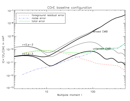
Figure 19: Forecasted errors on the CMB map due to foreground residuals (red dashed line), noise (blue dot-dashed line) and total (green solid line) for a linear component separation technique in pixel space (pix-LCS) assuming conservative errors on the recovery of the spectral model. Errors are compared to input CMB model with $r=(T/S)=5\times 10^{-3}$. Here mask 2 (a galactic cut with a smooth transition, corresponding to $f_{sky}\simeq 0.70$) has been used. The foreground rejection is good, but foreground residuals still dominate the error on large scales.

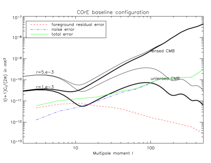
Figure 20: Same as figure 19, but errors are compared to CMB models with both $r=(T/S)=10^{-3}$ and $5\times 10^{-3}$. Here a more conservative galactic cut with $f_{sky}\simeq 0.65$ has been used (mask 3). The difference between the level of galactic residuals here and in figure 19 shows the importance of masking regions close to the galactic plane. The more conservative mask allows for very little residual foreground emission, adequate for measuring $r=0.001$.

3.4 Foregrounds and component separation: summary

Astrophysical confusion has become the major source of error for sensitive CMB observations. The development of component separation methods has become a very active topic in the context of the analysis of WMAP and Planck data. The design of COrE builds on the expertise developed for the previous space missions.

The complete spectral coverage provided by 15 different frequency bands is an important property of COrE. In any region where all components contribute (e.g. a galaxy cluster at moderate galactic latitude, with contamination by intra-cluster sources), or in regions with complex galactic foregrounds, all of these channels are needed for accurate characterization of all the emissions, which is an important part of the scientific programme of our proposed space mission.

This spectral coverage also important for securing adequate component separation for CMB science. Significant effort indeed is put into making COrE a very sensitive surveyor of the sky emission. For benefitting fully from the mission sensitivity, it is necessary that component separation be performed at an accuracy such that residual confusion is about as low as the noise level. This sets very demanding requirements for COrE: by reason of the very high S/N, component separation must be done to exquisite precision.

We have performed component separation and residual foreground contamination estimates specifically for measuring B modes with COrE, using for this PSM simulations which comprise polarised synchrotron and dust (both with emission laws varying over the sky), polarised point sources, and CMB. We show that a low level of primordial B-modes ($r=0.001$) is detectable with COrE, although this requires masking a substantial region of the galaxy. For higher values of $r$, we would gradually increase the sky coverage, for optimisation of the trade-off between cosmic variance and residual foreground contamination.

4 Science requirements

4.1 Sensitivity

The primary science goal of COrE is to investigate the physics at play in the early universe and to test extensively the standard cosmological model through high precision mapping of the CMB temperature and polarization anisotropies. Just as with previous CMB missions, this requires the sensitive measurement of sky emission in the millimeter wave domain where CMB emission is the strongest. It also requires additional channels to constrain and understand all astrophysical emissions contributing to the total sky emission. The level of polarization of CMB B modes from gravitational lensing, which is both an important scientific objective and an ultimate limitation for measuring primordial tensor B modes, is the main driver for the sensitivity of COrE. It sets the requirement that the COrE mission should measure sky polarization with a sensitivity better than 5$\mu$K$\cdot$arcmin in a set of frequency channels at the maximum level of CMB emission relative to foregrounds. The baseline COrE design includes among its fifteen frequency bands, six frequency channels between 75 and 225 GHz each having a sensitivity better than this requirement. This allows not only for the target sensitivity, but also provides the redundancy needed to check that the measured fluctuations indeed have the expected color of CMB fluctuations after these channels have been cleaned of foreground contamination.

The deployment of the detectors among the 15 frequency channels has not yet been optimized and should be studied further before a final configuration is fixed. For such optimization, which depends somewhat on the science goals and their relative priorities, there are essentially three constraints to be considered: focal plane area, cooling power, and telemetry rates. What performance can be expected for detecting B modes in the presence of galactic and extra-galactic foregrounds has been studied in Sec. 3. There we show what values of $(T/S)$ can be achieved for the present configuration. For the galactic science, the most important channel is the 795 GHz because it has the best angular resolution.

For the COrE Galactic science program, the goal is to map the Galactic polarization down to approximately one arcminute resolution to characterize the interplay between interstellar turbulence and the magnetic field in structuring the cold ISM. We want to probe the formation of $H_{2}$ clouds within the diffuse interstellar medium as well as pre-stellar cores in star forming molecular clouds. COrE will complement ground-based observations in a unique and essential way. Single-dish telescopes (IRAM, CCAT) and interferometers (NOEMA, ALMA) will map the magnetic field within compact sources on arcminute scales but will not be sensitive to extended emission.

Table 4 shows the polarization sensitivity of COrE for the emission from the extended envelopes of molecular clouds and bright clouds at high Galactic latitude (corresponding to a visible extinction of 1 magnitude). The sensitivity to the polarized fraction $\sim 1\%$ compares well with an expected polarization fraction that it is expected to vary across clouds within the range 3-15%. Data averaging over coherent structures in the intensity maps (e.g., interstellar filaments) will allow extending the CORE mapping of the Galactic polarization to fainter clouds at high Galactic latitude. The on-going analysis of PLANCK polarization data will allow us to sharpen the sensitivity requirements and decide on an optimal distribution of detectors among the frequency bands. We see that $S/N\mathrel{\raise 1.29167pt\hbox{$>$}\mkern-14.0mu\lower 2.58334pt\hbox{$\sim$}}7$ is achieved in a pixel of the highest-frequency channel, which has the highest angular resolution $(1.3^{\prime})$. In the last entry of the table we indicated the effect of increasing the number of detectors in the highest frequency channel by a factor of five relative to the previous baseline. It should be noted that for areas of very diffuse Galactic emission (H21cm emission of approximately $150~{}K~{}km~{}s^{-1}$), a signal-to-noise of approximately unity is achieved in a fwhm square pixel of the highest frequency channel (assuming a polarization fraction of 3% ).

				$(\Delta P)$/arcmin			Pixel sensitivity		$(\Delta P)_{A(V)=1}^{forecast}$
$\nu$	$\Delta\nu$	$n_{det}$	$\theta_{fwhm}^{arcmin}$	$(\mu{\rm K})_{thermo}$	$(\mu{\rm K})_{RJ}$	$MJy/st$	$(\mu{\rm K})_{RJ}$	$MJy/st$	$MJy/st$	$(S/N)_{pol}^{pix}$
255	15	575	4.10	$1.05\times 10^{1}$	2.43	$4.85\times 10^{-3}$	0.59	$1.18\times 10^{-3}$	$6.30\times 10^{-3}$	5.33
285	15	375	3.70	$1.74\times 10^{1}$	2.94	$7.33\times 10^{-3}$	0.79	$1.98\times 10^{-3}$	$8.20\times 10^{-3}$	4.13
315	15	100	3.30	$4.66\times 10^{1}$	5.62	$1.71\times 10^{-2}$	1.70	$5.19\times 10^{-3}$	$1.13\times 10^{-2}$	2.20
375	15	64	2.80	$1.19\times 10^{2}$	7.01	$3.03\times 10^{-2}$	2.50	$1.08\times 10^{-2}$	$2.12\times 10^{-2}$	2.00
435	15	64	2.40	$2.58\times 10^{2}$	7.12	$4.14\times 10^{-2}$	2.97	$1.72\times 10^{-2}$	$3.82\times 10^{-2}$	2.20
555	185	64	1.90	$6.26\times 10^{2}$	3.39	$3.21\times 10^{-2}$	1.78	$1.69\times 10^{-2}$	$7.53\times 10^{-2}$	4.47
675	185	64	1.60	$3.64\times 10^{3}$	3.52	$4.92\times 10^{-2}$	2.20	$3.08\times 10^{-2}$	$1.28\times 10^{-1}$	4.13
795	185	64	1.30	$2.22\times 10^{4}$	3.60	$6.99\times 10^{-2}$	2.77	$5.38\times 10^{-2}$	$1.65\times 10^{-1}$	3.07
795**	185	64	1.30	$1.00\times 10^{4}$	1.61	$3.13\times 10^{-2}$	1.24	$2.41\times 10^{-2}$	$1.65\times 10^{-1}$	6.86

^∗∗ represents the new modified baseline with the number of detectors in the 795 GHz channel increased by a factor of five as discussed in the main text.

Table 4: COrE performance for mapping polarized dust in the highest frequency channels. For the eight highest frequency channels for the baseline defined in Table 1, we indicate in three different ways the sensitivities scaled to an arcmin square pixel for the polarization $(Q,U)$ anisotropies, first as a thermodynamic temperature fluctuation relative to $T_{CMB}=2.73K$—that is, as a fluctuation in $\Delta T_{CMB},$ then as a Rayleigh-Jeans temperature fluctuation, and finally in terms of radiance units—that is, megaJansky per steradian. The polarization sensitivity is then given for a square pixel of dimension $\theta_{fwhm}$ on a side, as well as the prediction of the rms signal in Q and U in a pixel expected in a region with $A_{V}=1.$ Finally the resulting signal-to-noise within a pixel with unit magnitude visual extinction is indicated.

We propose to amend the baseline configuration defined in the proposal document submitted in December 2010 by deploying five times more detectors in the 795 GHz channel. What is required to effect this increase would take away a small part of the focal plane from the central ‘primordial cosmology’ channels and thus will leave intact the primordial cosmology capability forecasts. In the former baseline configuration the detectors devoted to the 795 Ghz channel occupy less than 1% of the focal plane area and contribute less than 4% to the data rate. Therefore their number could easily be increased by a factor of five with only modest reductions in the other channels. The keep the data rate transmitted to Earth down, one could also study the option of placing five detectors one behind the other in the scan direction so that on-board compression could be used to keep the data rate unchanged.

4.2 Angular resolution

The observation of the primordial tensor CMB B-mode spectrum nominally requires only a modest resolution, of order 1^∘ on the sky, significantly lower than already achieved by WMAP and PLANCK. CMB lensing, however, generates deflections of order 2.7 arcminutes. Since the lensing signal is concentrated on the smallest scales of the survey, one wants to sample the primordial CMB with S/N of approximately unit on as small scales as possible where foreground removal is feasible. Beyond the COrE resolution one rapidly enters into the Silk damping tail and contamination from compact sources rapidly becomes dominant. With its resolution COrE is sensitive to the interesting range of absolute neutrino masses suggested by current neutrino oscillation data.

For Galactic science, the high resolution mapping of the galactic magnetic field in star-forming regions is the key for understanding the interplay between turbulence and magnetic field, which leads to the formation of pre-stellar condensations. A resolution of order 1 arcminute is adequate to complement what can be done from the ground with ALMA and single dish sub-mm telescopes, which will provide polarization imaging at sub-arcminute angular scales of a variety of compact sources including pre-stellar condensations.

As a final constraint, we note that galactic and extragalactic point sources can be a significant contaminant for measuring CMB B modes, should the tensor-to-scalar ratio be low. As each point source has its own emission spectrum, this contamination cannot be effectively removed using multi-frequency observations unless the sources can be isolated in the maps. This calls for the best possible angular resolution, which sets the lower limit on the flux limit of detectable point sources.

A limiting constraint for the COrE resolution, however, is set by the diffraction limit due to the size of the telescope (set in turn by the size of the fairing for a space mission). We thus require the highest possible resolution available from space, and demonstrate, as discussed in the science section, that it is adequate for achieving the main science objectives of COrE.

4.3 Control of systematics

Rigorous control of systematic effects is an essential requirement for any experiment aiming to measure CMB polarization. Systematic effects are essentially of two kinds. Additive errors (such as glitches due to cosmic ray impacts, stray signals due to temperature drifts of the payload, low frequency noise), and multiplicative errors (errors on the instrumental response such as inaccurate beam shapes, unknown cross polarization leakage, sidelobes in the optical response, gain drifts). Minimizing such systematics requires both a very careful instrument design and the capability to measure instrumental imperfections in flight.

Extensive simulation of the impact of systematic effects on polarization measurements has been carried out for PLANCK and for the US EPIC project. This work has determined the limits needed on gain mismatch and beam asymmetry and have been taken into account in the COrE instrument design. In addition, COrE mission provides four layers of redundancy: at the detector level through polarization modulation, which provides coverage of many polarization angles by the same pixel viewed with the same detector while keeping the telescope attitude fixed with respect to the sky and thereby rejecting systematics fixed with respect to the spacecraft; at the scanning strategy level through a tightly connected coverage of the sky resulting from a well designed scanning strategy allowing the same detector to revisit the same sky pixel at different time intervals; at the band level, through many different detectors observing the same sky pixel over different time intervals; at the focal plane level, through six CMB sensitive frequency channels. This many levels of redundancy offer many tests for unexpected systematics, and many ways to correct for them.

4.3.1 Additive errors

Previous experience from PLANCK HFI demonstrates that cosmic ray hits can be detected, and their effect can be subtracted from bolometer timelines [258]. The effectiveness of such data correction depends on the rate of cosmic ray hits to be taken into account in each bolometer time stream (too many of them results in blending of the glitches). As most of the improvement of sensitivity between PLANCK and COrE comes from the increased number of channels (rather than from the sensitivity of the individual detectors themselves, which is nearly photon shot noise limited), the PLANCK experience for glitch correction can be adapted to COrE without major change.

Similarly, low frequency noise in bolometer timelines will be kept low enough, so that the so-called “knee frequency” (at which low frequency noise starts being dominant) will be lower than the typical modulation frequency provided by the RHWP and the scan strategy. As discussed by numerous authors in the context of the PLANCK mission [232, 260, 254, 249, 219, 220, 251, 250], this measure will allow almost complete suppression of residual low frequency noise after data processing to produce maps of temperature and polarization. Most other additive errors induce signals which are either very sparse (e.g., microphonic lines) or very low frequency (e.g., thermal drifts) and can be dealt with similarly in a data analysis stage.

4.3.2 Multiplicative errors

Multiplicative errors have been identified as a potential source of error for measuring CMB polarization. This category includes all errors in characterizing the detector response: calibration, beam shape, band shape, transfer function, detector orientation, pointing, depolarization (or cross-polarization leakage), etc. In essence, the problem is that each detector measures a linear combination of three Stokes parameters $I$, $Q$ and $U$. Coefficients of the linear combination depend on the detector response. The recovery of all Stokes parameters requires combining measurements from either different detectors, or from the same detector, but with a different orientation (or different polarization angle as set by the RHWP). This linear combination of different measurements is an inversion of a linear system which connects measured quantities to sky temperature and polarization. If the coefficients in the linear system are not well known, the inversion is imperfect, and the measured Stokes parameters still contain admixtures of unwanted components. Because of the strong hierarchy in power among $I$, $E$ and $B$, these errors induces leakage of $I$ into $E$ and $B$ (from errors in calibration, beam, frequency bands, etc.), and of $E$ into $B$ (e.g., from polarization orientation errors) [248, 246].

This potentially severe problem has been identified during the preparation of the PLANCK mission and has motivated method papers to handle the problem during the data analysis stage [262] as well as several studies for defining the EPIC mission proposal in the US [263, 256]. While detailed studies of the problem for COrE specifically will be part of the ongoing activities for the preparation of the space mission, the COrE design takes into account the experience already gathered on these issues. The RHWP provides a selection of the polarization as the first optical element, which contributes to the cleanliness of the measurement. As a second step, data processing has been shown to allow correction of effects to first order. Finally, the many detectors provide an effective averaging of imperfections (an effective averaged beam from 1000 detectors is more symmetric than the beam from a single detector) as well as redundancy to check that all measurements agree.

To take a simple example, current measured beams have an ellipticity of order 5%, well above the requirements for an accurate measurement of the CMB $B$ modes [256]. Both instrumental optimization and the RHWP, however, can reduce this ellipticity (or its impact on the measurement) by a factor 2–5 at least. Corrections during the data analysis stage can gain an order of magnitude, as shown for PLANCK in [262]. The averaging of residual errors from O(400-1000) detectors gains another factor 20-30, for a final beam ellipticity effect of order 400 to 1500 times lower (of order $2-6\times 10^{-5}$), well within requirements for the measurement of primordial and lensing B-modes.

4.4 Why space?

Balloon experiments such as EBEX and SPIDER along with ground-based telescopes such as PolarBear and SPT ), with thousands of detectors in one or two frequency bands and sufficiently long integration time, are just now reaching levels of instantaneous sensitivity to achieve white-noise levels of $3\mu K$ per arcminute at a single frequency, arguably sufficient to reach $r\simeq 0.05$ in the absence of contaminating systematics, with angular resolutions varying from ten arcmin to one degree. These experiments have already demonstrated the technical feasibility of measuring the CMB with thousands of detectors.

However the full science goals outlined above require a yet higher sensitivity to cosmological and astrophysical polarization over a wider range of angular scales and frequencies. To realize this program in practice requires control of systematics at a level that cannot be achieved in suborbital experiments. A satellite experiment like COrE is therefore a necessary next step. COrE will observe the full sky at multiple bands spanning over a decade in frequency and take data for very long integration times in the very quiet environment of the L2 Lagrange point of the Sun-Earth system.

4.4.1 Full sky coverage

COrE’s science goals are best achieved with high sensitivity over the full sky. Full-sky coverage will enable measurement of the reionization signal in polarization, which is crucial for confirmation of the last-scattering B-mode signal at medium scales. Moreover, full-sky coverage will accumulate sufficient signal-to-noise for the non-Gaussian signal, constrained by the number of independent triples (or quadruples,$\ldots$) of modes available. Full-sky coverage will be crucial if we want to go beyond detection of $f_{\textrm{NL}}$ to detailed non-Gaussian models of the higher-order moments as discussed above.

Situated between the strongly radiating ground and Sun, suborbital experiments are highly constrained in the amount of sky that they can observe as well as how they can observe it. They must scan at constant elevation to avoid rapidly-changing ground pickup while simultaneously avoiding the Sun. Hence these experiments can typically observe a maximum of a few thousand square degrees with only mild cross-linking of different scans, with details strongly dependent upon the location of the experiment.

4.4.2 Avoiding the atmosphere

The atmosphere allows observation in just a few atmospheric windows, incompatible with the wide frequency coverage required to fulfill the scientific objectives of COrE. If only for this reason, COrE must be a space mission. Even for less ambitious science goals, the atmosphere turns out to be a severe problem for polarized CMB observations from the ground. The atmosphere indeed is a strong source of microwave emission. Although largely unpolarized, the atmosphere adds to the photon shot noise, reducing detector sensitivity and hence making necessary longer integration times. Moreover, Zeeman splitting due to the Earth’s magnetic field leads to both linear and circular polarization. The linear polarization may be small $(\approx 10\textrm{nK}$), but the circular polarization is much larger $(\approx 10^{2}\mu\textrm{K})$, and great care must be taken to avoid conversion into linear polarization within the instrument. Another effect leading to significant polarization is the back-scattering of thermal radiation from the hot ground by the atmosphere. This results primarily from large ice crystals (i.e., 100–1000 $\mu\textrm{m}$) in high-altitude clouds, often optically thin (along with a smaller effect from molecular scattering). Simulations demonstrate that at both the South Pole and in the Atacama desert such polarized emission will likely swamp the B mode signal from primordial tensor modes. [Pietranera2007].

4.4.3 Benign environment (especially L2)

Even with highly constrained, constant elevation scans, suborbital experiments would need to reject far sidelobes from the $250\;\textrm{K}\times 2\pi\;\textrm{sr}$ ground at a level of roughly $10^{-10}$ to remain below the desired noise on large angular scales. From a distant point in space such as L2, the Earth will instead subtend an angle of only $0.5^{\circ}$, reducing its emission by a factor $10^{5}$. Moreover, at L2 the Earth, like the Sun, can be more easily shielded, limiting the emission from both to diffraction around (and temperature variations within) the shielding.

These same considerations apply to temporal variations in the ambient temperature, which can be up to several degrees per day on Earth at mid-latitudes, compared to the nearly completely stable environment in space. For COrE, any change in thermal loading is due to the behavior of the cooler itself and can be strictly controlled and monitored, as well as kept to specific times during the mission.

One potential worry in deep space is the increased flux of cosmic rays. The rates at L2 for high-sensitivity bolometers have been measured by PLANCK HFI and while not negligible, do not prevent PLANCK from reaching (and indeed surpassing) its sensitivity goal. Hence the achieved PLANCK detector sensitivity gives the proper estimate for COrE, multiplied by the vast increase in detector numbers. We are thus very confident that any extra noise induced by cosmic rays will not challenge the COrE sensitivity goal.

The L2 environment also allows much longer integration times than can be achieved from balloons (with an ultra-long duration limit of roughly 40 days at present) and a higher duty cycle than ground-based experiments.

Only from space can an experiment like COrE achieve its simultaneous goals of full-sky measurements of astrophysical polarization over a decade in frequency and an angular resolution of a few arcmins, and $\mu{\rm K\cdot arcmin}$ sensitivity coupled with thermal stability and $10^{-5}$ sidelobe rejection.

5 Proposed COrE instrument

The technology deployed for the PLANCK mission is performing exceptionally well as reported in the papers released in January 2011 [289, 290], and breakthrough science is in the process of being delivered. Although the cosmological results are still being analyzed, the quality of the data collected has been characterized and documented in these papers [272]. Much of the technology of the COrE instrument has already been tested on PLANCK and the expertise accumulated from PLANCK will be of great value for COrE. COrE builds on the PLANCK and Herschel heritage and on the experience gained from a generation of suborbital experiments. In order to reduce the risks and develop an instrument in a timeframe compatible with the next ESA M3 mission, COrE builds on the subsystems from PLANCK. The optical system, the passive as well as some of the active cooling system and most of the service module use the same technology, leading to a payload with similar characteristics (mass, volume power budget and cost) as shown in Table 5. Moreover, whereas PLANCK was based on two different detector technologies leading to instruments with two separate focal planes—the LFI instrument based on HEMT technology and the HFI instrument based on bolometers—, COrE uses the same technology for all its spectral bands, reducing the risks associated with potential incompatibilities and integration problems.

The great advance in science output from PLANCK to COrE is made possible by a massive increase of number of detectors. COrE will have altogether about 6400 detectors whereas PLANCK only has 71 detectors. The use of large arrays of dual-polarized detectors divided in 15 spectral bands ranging from 45 to 795 GHz allows for this massive increase. The resulting performances have already been summarized in Table 1 in the Introduction. The spatial resolution ranges from 23 arcmin to about 1.3 arcmin for the highest frequency band with a Q and U sensitivity of about 4.5 $\mu{\rm K}\cdot$arcmin in each of the main science channels.

Another key difference with respect to PLANCK is the presence of a polarization modulator as the first element in the optical chain. For the massive increase in raw sensitivity to be useful, it must be matched by a corresponding improvement in the control and characterization of systematic errors. Unlike PLANCK, in COrE the incoming polarization is modulated using a common single rotating reflective half-wave plate. In this way, most of the systematic errors arising within the telescope as well as those involving issues of control of the beam profile are modulated away. While the rotating half-wave plate does add some complexity to the system, its presence allows requirement on other aspects of the system to be relaxed. The SAMPAN design, for example, lacked modulation but instead endeavored to control systematics using a complicated and difficult to realize scanning strategy.

The main challenges of the COrE design arise from the development of the focal plane components and the implementation of the polarization modulator. Several European institutes also supported by industry are able to produce the elements constituting each pixel (the feedhorn, orthomode transducer (OMT), and the bolometric detectors) as detailed in the following sections. The production of the large number of pixels will be ensured by parallel production of the various components.

5.1 COrE instrument overview

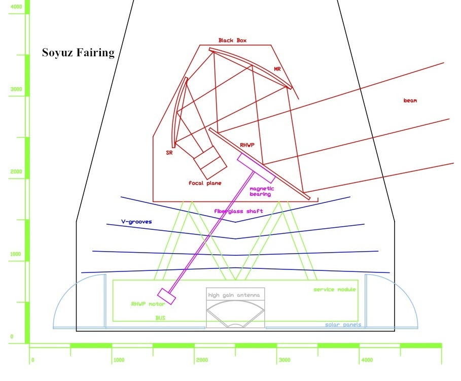
Figure 21: Sketch of the Soyuz fairing including the COrE payload

The instrument (Fig. 21) uses an off-axis reflective telescope capable of providing a large focal plane area (Fig. 22 left) with limited aberration and cross-polarization. For reasons explained in Sect. 5.3.2, polarization modulation is achieved using of a reflective half-wave plate (RHWP) located at the aperture of the telescope. The RWHP modulates away or minimizes many of the systematic errors that must be overcome for high precision polarization measurements. After reflecting off the RHWP, the incoming radiation passes through the telescope and is focused onto the detector arrays. While technology based on planar detector arrays has made tremendous progress [273] (used in BICEP2 for example), in order to reduce the risks associated to the lack of maturity, COrE uses feedhorn-coupled detectors. Horns have the advantage of defining a well-formed beam with rapidly decaying far sidelobes. These horns are coupled to ortho-mode transducers (OMTs) through a circular waveguide while each branch of the OMTs separating the two linear polarizations is coupled to a bolometric detector. The cold optics (feedhorns+OMT+detector pair) are cooled to 100 mK and surrounded by several successive temperature stages. The whole instrument is enclosed by a passively cooled 35 K shield. The telescope mirrors and the RHWP could reach a temperature as low as 30 K. Table 5 gives the overall characteristics of the payload as a comparison to the Planck mission.

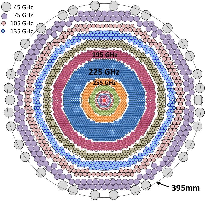
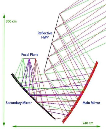
Figure 22: Left: Focal Plane Unit. The highest frequency band (795 GHz) is at the center and the 45 GHz horns are at the periphery. Right: Ray tracing of the optical system showing the off-axis telescope and the RHWP.5

Table 5: COrE payload summary table compared to PLANCK. The full payload includes the service module and hydrazine. The data transfer rate of COrE assumes a compression factor of 4 and a 2 hours per day downlink.

	COrE	PLANCK
Overall mass	1832 kg	1974 kg
Power budget	1279 W	1342 W
On-board data storage	780 Gbit	32 Gbit
Data transfer rate	54 Mbit/s	1.5 Mbit/s

5.2 Description of the measurement technique

COrE will carry out a full-sky measurement of temperature anisotropies and polarization of the CMB. The choice of a far-Earth orbit, such as a halo or a quasi-periodic Lissajous orbit around the Sun-Earth Lagrangian point L2, is a requirement for COrE in order to provide sufficient control of straylight contamination from far sidelobe pick-up. Requirements for far-side lobe rejection are extremely stringent for COrE. Because the gross features of the beam pattern at large off-axis angles are essentially the same for all detectors at a given frequency, the required rejection must be calculated against the total sensitivity per frequency channel. Using the PLANCK requirements as a guide, and assuming a factor of 10 better sensitivity for COrE in an L2 orbit, we need roughly -110 dB rejection for contamination from the Sun, -100 dB contamination from the Earth, and -80 dB contamination from the Moon. Stringent, highly frequency-dependent rejection requirements will be imposed also by straylight from diffuse galactic emission entering via the intermediate side lobes. Although challenging, these straylight rejection requirements for COrE can be achieved with a very careful optical design and can be tested with a moderate extrapolation of the state-of-the-art technology developed by ESA for the PLANCK mission. Furthermore, the excellent thermal stability of the L2 environment is ideal to minimize thermal systematic effects on the instrument. The experiences of both WMAP and PLANCK have demonstrated exquisite thermal stability against small changes in the solar aspect angle, with very small and slow residual thermal drifts.

From the data analysis point of view, we need full sky coverage to optimize the redundancy in each map pixel and the range of timescales for revisiting a given pixel in order to reject “naturally” the statistical noise and most common systematic errors. Moreover, polarization determination requires a wide variety of measurement angles per pixel. In the first B-Pol proposal, all the polarization modulation efforts involved payload motion. This led to a sophisticated (but feasible) scanning strategy and set tight constraints on sun shielding. For COrE, the addition of a HWP modulator relaxes these requirements and allows for a scanning strategy similar to PLANCK, with only a precession of the spin axis and possibly some level of nutation. If the COrE spacecraft is a ‘spinner,’ the spin rate $\dot{\mu}$ must be fast enough to ensure redundancy to minimize $1/f$ noise and thermal fluctuations yet slow enough to be compatible with the bolometer time constants. A ‘spinner’ is a spacecraft with a nonvanishing total angular momentum that is periodically re-oriented using thrusters. The alternative is a three-axis stabilized spacecraft with counter-rotating flywheels allowing for more complicated manoeuvring with essentially no energy expenditure owing to the fact that the total angular momentum is nearly zero at all times. Based on the PLANCK experience, we envisage a spin rate of order 0.5 rpm, and a step and point approach for the spin axis like in PLANCK, with similar telescope de-pointing. This means that the spin axis would be fixed for certain time allowing for a few rings, then moved to another direction and kept fixed to allow for a few rings and so on. The difference $\Delta\phi$ between two consecutive spin axis positions would be of 1 to a few arcmin every few tens of circles and therefore maintain the nearly anti-solar configuration ($\Delta\phi/\Delta t\sim 1^{\circ}$/day). This would yield sufficient redundancy in sky circles and, simultaneously, good sampling of the sky for each single beam up to 220 GHz (i.e., in all the main COrE cosmological channels). At higher frequencies, where the angular resolution is $\theta_{fwhm}<4$ arcmin, adequate sampling would be ensured by proper staggering of the feeds in the focal plane.

Tight constraints are imposed on the scanning parameters to avoid thermal and stray light artifacts and by data transmission requirements. The maximum excursion $\alpha$ of the spin axis from anti-solar direction must not exceed $27.5^{\circ}$ to avoid thermal effects and straylight contamination from the Sun and Moon and to prevent power modulation due to spacecraft asymmetries or shadowing of the solar panels. Moreover the angle between the spin axis and the Earth direction must remain below $20^{\circ}$ to ensure adequate visibility of a fixed medium gain antenna for telemetry activity. While steerable antenna designs are possible, we do not favor their use since they would complicate the design and increase risk. Depending on the dynamical constraints and attitude control capabilities, modulation of the spin axis can be set either by precession (with the advantage of maintaining a constant solar aspect angle or with cross-ecliptic excursions at an angle $\alpha=90-\beta$. The optimal configuration will be determined via simulations that include polarization angle redundancy, de-striping efficiency, and figures of merit for straylight and thermal effects. Table 6 summarizes a possible baseline based on the PLANCK experience.

Table 6: Scan parameter definitions and allowed variations

Parameter	Definition	Range	Potential criticalities
$\beta$	Telescope axis	$65-85^{\circ}$	$>85^{\circ}$: stray light, polarization angle redundancy
	to spin axis angle		$<65^{\circ}$: excessive excursion $\alpha$ angle required
$\dot{\mu}$	Spin rate	$0.1-2$ rpm	$<0.1$ rpm : $1/f$ noise, thermal fluctuations
			$>2$ rpm : bolometer time constant
$\Delta\phi$	Depointing angle	$1-$few arcmin	$<1$: limited redundancy in sky circles
			$>2$: insufficient sky sampling
$\alpha$	Solar aspect angle	$5-27.5^{\circ}$	$<5$: coupling with $\beta$ and full-sky requirement
			$>27.5$: thermal effects, stray lights
$\psi_{Earth}$	Maximum Earth	$0-15^{\circ}$	$>15$: TM/TC requirements
	aspect angle
$\dot{\phi}$	Precession frequency	1-24 weeks	polarization angle redundancy, destriping
			thermal effects

A three-axis stabilized satellite would allow improvement of the scanning strategy concept above. One could, for instance, imagine combining the best of the PLANCK and WMAP scanning strategies by superimposing a daily nutation of $20\nobreak^{\circ}$ about the antisolar direction, bringing the spin axis back to the anti-earth position every 24 hours. This would distribute the basic ring measurement to fill an $\sim$ $40\nobreak^{\circ}$ annulus. The same pixels would be revisited several times over a 40 day interval (constraining systematics of differing periods) at the expense of somewhat uneven sky coverage. Optimization is left as an option for further study.

In addition to the classical compromise between survey size and sensitivity, COrE has to account for the directivity of polarization. It is both an additional constraint on the system and a lever arm against systematic effects. Polarization is usually described in terms of the Stokes parameters $I$, $Q$ and $U$. In COrE we propose to implement a polarization modulator made of a rotating half-wave plate (hereafter RHWP) which modulates simultaneously all the detectors in the focal plane, so that each detector measures

$$m=0.5(I+Q\cos 4\alpha+U\sin 4\alpha)+n$$ (23)

where $n$ is the noise and $\alpha=\omega t$ the orientation of the RHWP. Each measurement is the linear combination of three independent parameters. Three independent measurements, each at a different angle $\alpha$, are therefore required (at least) to determine the polarization state. In the absence of a polarization modulator, these measurements would require rotating the detector. However that approach contaminates the sought polarization signal with beam shape and detector related artifacts. Introducing the modulator very significantly simplifies the measurement and scan strategy. The satellite no longer needs to be rotated, and the sky scan can be very similar to that of PLANCK. The continuous rotation of the RHWP at a frequency incommensurate with the spin frequency provides the required change in $\alpha$ for each reobservation of the same sky pixel. After three rotations, a ring of fully determined $I$, $Q$, $U$ has already been obtained. Further rotations serve to improve signal-to-noise and to remove systematics. The idea behind this modulated measurement, as eqn. 23 shows, is that polarization is modulated at $4\alpha$ when the modulator is rotated by $\alpha$, whereas most systematic effects are fixed in the instrument reference frame. Rotating the modulator with respect to the incoming polarization and providing sufficient angular coverage is therefore analogous to a lock-in detection that selects polarization and cancels out systematic effects. The rotation frequency of the modulator is around 0.1–0.5 Hz.

Results of detailed simulations of this scan and modulation strategy are summarized in Fig. 23. The improvement compared to PLANCK (which was not optimized for polarization measurements) is substantial. To illustrate this point, we chose typical PLANCK parameters ($\alpha=5^{\circ}$, $\beta=85^{\circ}$, $\dot{\mu}=1$ rpm) with a continuous rotation (1Hz). For these simulations, we assumed standard white noise and $1/f$ noise with $f_{knee}=0.1$Hz and a $NET=10\mu\rm{K\cdot sec}^{1/2}$.

A detailed optimization of scan parameters (angles and precession and nutation frequencies) deserves to be studied. At present we conclude that the presence of the HWP enables COrE to relax previous requirements concerning sun-shielding and the scanning strategy. Our single detector simulations show that a continuously rotating HWP rejects $1/f$ noise better than a stepped HWP. However, we stress that (1) $1/f$ rejection can be addressed using high-performance de-striping algorithms such as those developed for PLANCK, and (2) stepping the HWP enables fine tuning of the angular coverage and could provide a significant technical simplification.

Moreover, we have some estimates about some of the instrument parameters, more specifically about the satellite spin rate (0.5 rpm) and the RHWP rotation speed (0.1 to 0.5Hz) derived from either present experiments or preliminary simulation results. A more precise value of these parameters will require further study. However the sub-systems concerned are studied to accept a range of values which will be compatible with an improved scanning strategy.

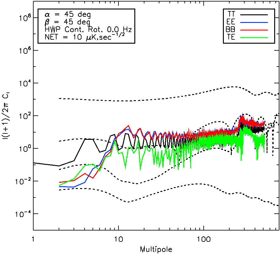
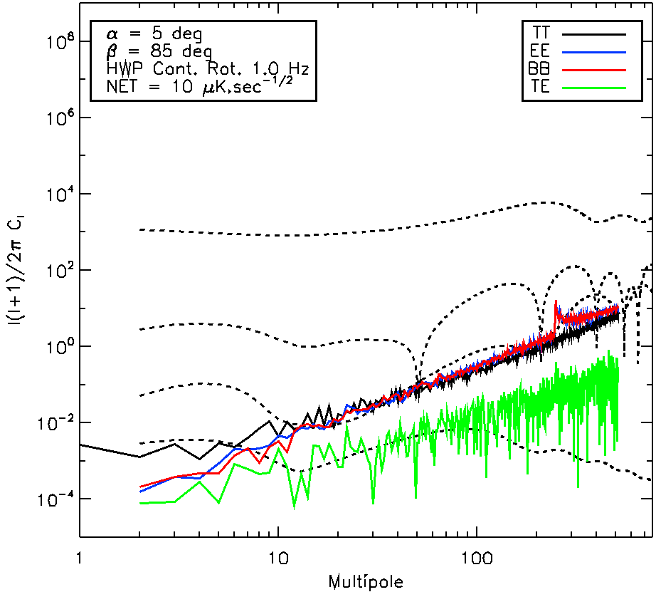
Figure 23: Angular power spectra of the $1/f$ noise timelines. Previous B-Pol proposal without HWP (left), PLANCK and continuously rotating HWP at 1Hz (right).

5.3 Instrument subsystems description and technology

5.3.1 Optical and RF configuration

The specifications required for achieving the scientific goals of the mission relating to the optical design are the resolution, edge taper and spillover, beam ellipticity (requirement$<1\%$), and cross-polarization (requirement $<-30$ dB). To meet the requirements using high Technology Readiness Level (TRL) technology within the size and weight budgets of a Soyuz launcher, we have chosen a payload with a single reflective off-axis compact test range telescope configuration (such as for ground-based Clover [274] and QUIET [275] projects) following the Dragone-Mitsugushi configuration. Used in conjunction with feedhorn-coupled detectors, this design allows for a large focal plane unit (FPU) with limited aberrations necessary to fulfil the scientific requirements. This technology is already rated TRL 9. However because of the large number of detectors, further development is required, mainly to reduce the mass, cost, and complexity and to ensure reliability. To limit the dimensions of the FPU, the horn apertures need to be small, resulting in a fast optical system. The resulting configuration has a 1.2 m projected diameter making use of large field of view horns (F2 aperture number), each having a 3$\lambda$ aperture diameter. Taking into account an array filling factor of 0.8 and leaving enough space for the spectral filtering, the overall FPU diameter is about 40 cm (Fig. 22 right). The entire optical system is enclosed in a cavity formed by a shield at 35 K with the RHWP acting as a cold stop. The telescope could reach a temperature as low as 30 K with passive cooling (compared to 50 K on PLANCK).

While this first iteration optical concept is already producing good performance, improvement will be needed as an outcome of a Phase A study. While the cross-polarization of the whole system is predicted to be within the requirement, attention will have to be paid to the beam ellipticity which could be improved with a lengthy optimization of the telescope and RHWP designs as well as a reshaping of the FPU surface (curved instead of flat as assumed so far).

In the present unoptimized design, when the uniformizing effect of the RWHP (see § 5.5) has not been taken into account, the beam ellipticity ranges from below 0.5% to about 5% for the edge pixels (depending on frequencies and location in the focal plane). Most of the pixels having an ellipticity of about 3%. For comparison, PLANCK beam ellipticities range from 5% to about 15% [279], [280]. Also the possibility of having a colder RHWP will be investigated to reduce the spillover contribution and to limit the effects of its emissivity (§  5.3.2).

The feedhorn transmits the full intensity of the incoming radiation through its circular waveguide onto an OMT that separates the two linear polarizations. The horn-OMT assembly determines the minimum cross-polarization achievable between the two branches that guide each polarization to the detector. Waveguide OMTs are the best. Return loss and isolation of order -20 dB and -50 dB, respectively, have been already achieved at 100 GHz for a 30% bandwidth [282], and -40 and -70 dB, respectively, at 30 GHz. Although further development is underway, this TRL 9 technology is potentially too heavy, and so far allows similar performances only for frequencies below 150 GHz. For this reason the OMT baseline adopted relies on planar technology.

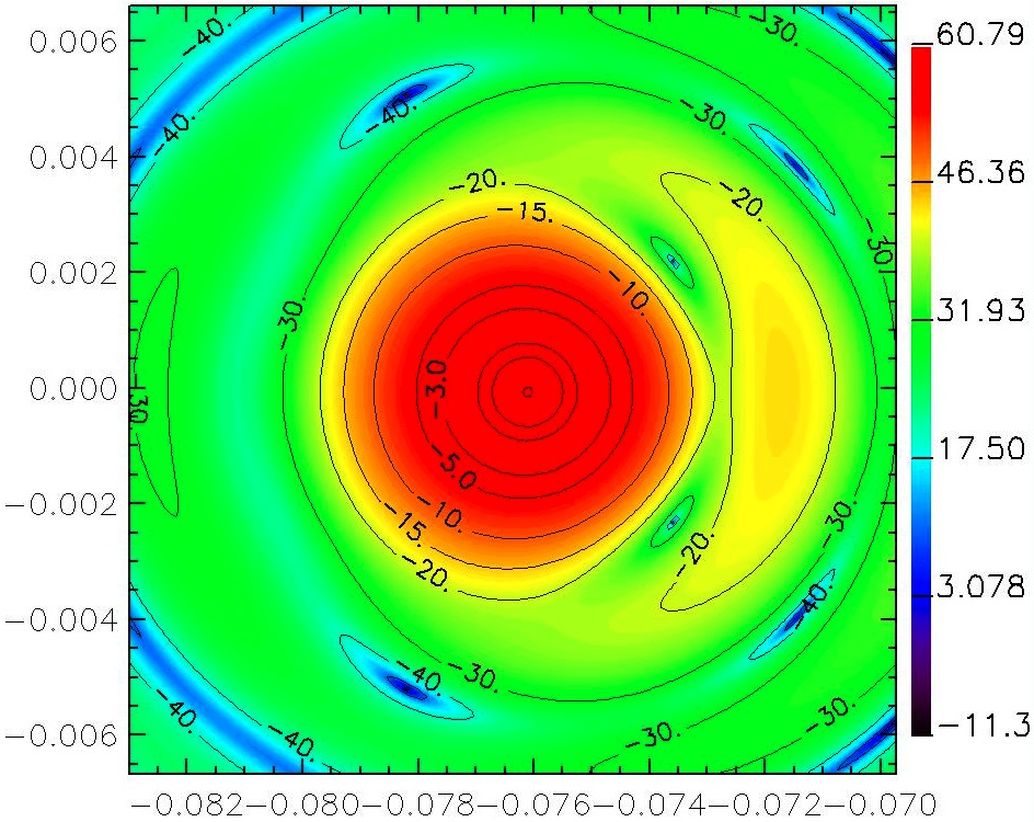
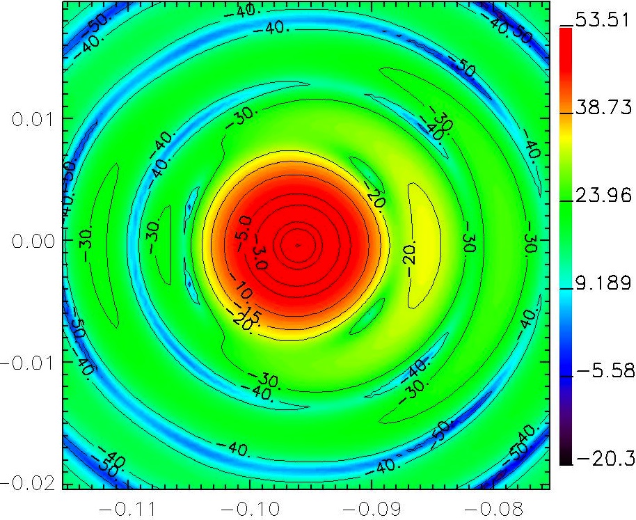
Figure 24: GRASP beam simulations in the U-V plane for two extreme off-axis pixels. (right) 45 GHz, (left) 105 GHz. Both have 5% beam ellipticity. Optimization to reduce the beam ellipticities will be carried out during the Phase A study.

Mirrors:

The PLANCK telescope has demonstrated that the technology needed already exists [291]. The mirror is fabricated using a carbon fiber reinforced plastic (CFRP) honeycomb sandwich technology and is coated with a thin reflective layer of aluminium. With dust contamination taken into account, the emissivity of the mirrors should not exceed 0.5%, even for the highest frequency band (857 GHz). The surface quality is satisfactory; however, if even higher quality is required, other technologies such as the one used for the Herschel telescope are also rated at TRL 9.

Feed horns:

Corrugated horns are extensively used in CMB experiments due to their very high performance. They exhibit very high polarization purity and low sidelobes levels, and the corrugation profile can be adjusted to meet electrical and mechanical requirements as well as to control the phase center location. However corrugated horns are slightly heavier and more difficult to manufacture than smooth walled horns due to the definition and thickness of the corrugations. This leads to potential problems for large arrays of closely packed horns. Different solutions are in development at various institutes.

The University of Oxford is developing smooth walled horns (Fig 25 center) that are drilled to have a chosen profile [277] giving performances nearly as good as corrugated horns. These performances might be good over a reduced bandwidth but large enough still to match COrE spectral bandwidths. Most the development effort seeks inexpensive and reliable ways to manufacture lighter corrugated horns. As an example, we mention the platelets technique used by the QUIET experiment (US), also developed in Italy (University of Milano - Fig. 25 left) and France (APC - Paris). While the manufacturing process is simplified and less expensive, mass reduction still needs improvement. For that purpose, previous development efforts produced horns made of metal coated Kevlar (Fig. 25 right) which have been successfully flown (Italy/UK). Also, the University of Wisconsin has recently manufactured a 100 GHz prototype corrugated horn made of metal coated plastic with good RF characteristics for a first attempt through stereolithography techniques. Further development is needed in order to test its cryogenic performance.

Within a few years these techniques should reach the level of maturity required for incorporation in the final instrument design.

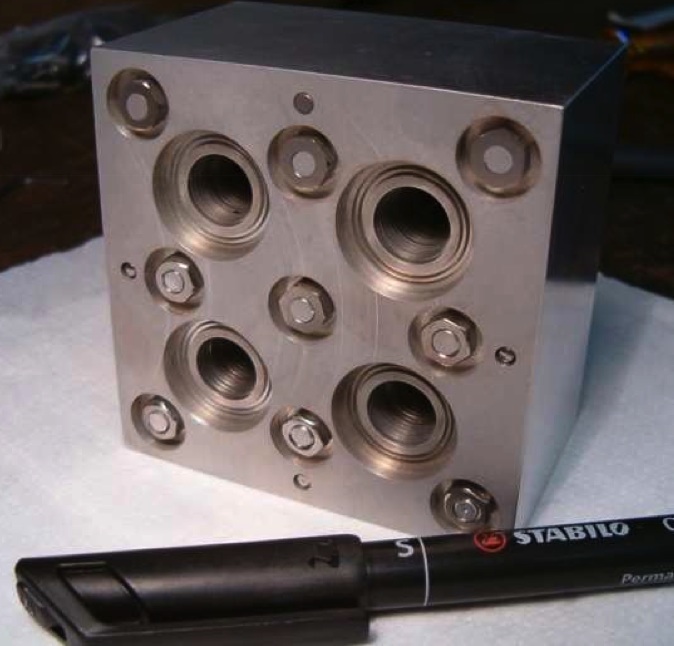
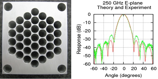
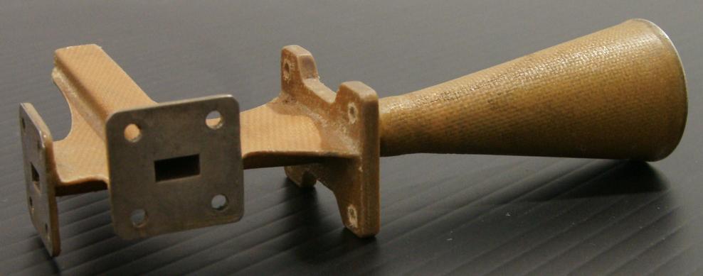
Figure 25: Left: array of platelets horns (University of Milano, Italy). Center: array of drilled smooth walled horns together with a measured beam pattern (University of Oxford, UK). Right: combined horn and OMT made of Kevlar as a monolithic piece. The inside is coated with metal.

Polarization separation:

Several countries in Europe and the US are developing planar OMTs, some of which are now being used in experiments. Models shows that return loss of the order of -20 dB with an isolation of about -50 dB is possible (measured for the C-BASS project at 5 GHz [278]). However similar results have not yet been confirmed experimentally at high frequencies (above 100 GHz). While planar OMT technology seems the most promising, it needs improvement, and other techniques will need to be investigated if planar technology subsequently proves to be inadequate. Parallel to horn fabrication R&D, efforts are underway to simplify the manufacture of waveguide components while retaining their exceptional RF performances. Platelets technology can also be applied to OMTs for which spark erosion manufacturing tolerances reache a few microns making possible the extension to high frequencies.

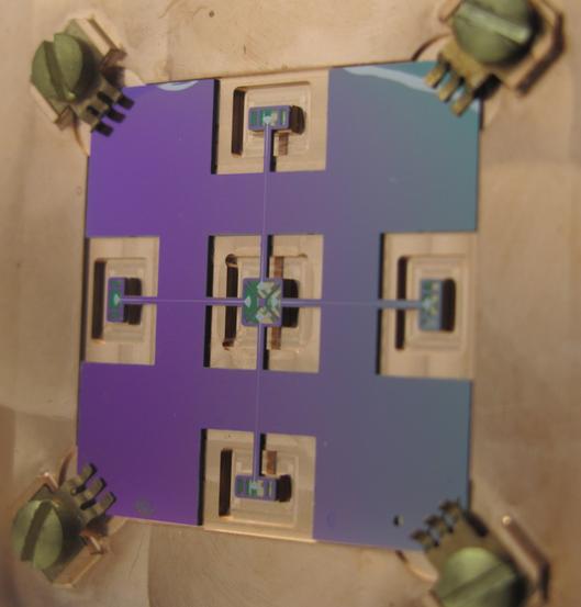
Figure 26: Left: prototype of 100 GHz planar OMT (Fr). Right: Clover 97 GHz waveguide OMT (UK).

5.3.2 Polarization modulator

A traditional transmitting half-wave plate [281] cannot cover the full COrE spectral range. It is important that the polarization modulator be placed as the first element of the optical chain, closest to the sky. Otherwise systematic errors remain that are not modulated away. This consideration excludes a single telescope with many polarization modulators, each tailored to a specific frequency range. The alternative would be to use several telescopes, but since size is a prime cost driver for an instrument of fixed physical size this option would entail unacceptable degradation of the angular resolution. We have therefore chosen to use a reflecting half-wave plate (RHWP) consisting of a free-standing wire grid polarizer held at a fixed distance $d$ from a flat mirror (Fig. 27). The RHWP rotates aibout an axis orthogonal to its surface and passing through its center. With the RHWP oriented as in Fig. 27, the RHWP introduces a phase shift between the two orthogonal ‘s’ and ‘p’ polarizations (orthogonal and parallel to the plane of incidence, respectively) that depends on the angle of incidence $\phi.$ When the phase shift is $180^{\circ}$ and the RHWP rotates with angular velocity $\omega,$ the overall effect is a rotation of the reflected linear polarization at a frequency $2\omega$. This happens only when the path difference between the two waves is equal to $\pi$—that is, at the frequencies

$$\nu_{n}^{RHWP}=(2n+1)\nu_{0}^{RHWP}\qquad{\rm with}\qquad\nu_{0}^{RHWP}=\frac{c}{4\cos(\phi)d}$$ (24)

where $n$ is an integer and $c$ the speed of light. The modulation efficiency is a sinusoidal function of frequency with maxima at frequencies $\nu_{n}$. Without spectral filtering, the average modulation efficiency is 0.5. With spectral filtering (to be implemented, see § 5.3.4), higher efficiencies can be achieved in narrower bands. A window of 50% bandwidth around one of the peaks gives an efficiency of 80% . In our case, this means that the bandwidth of each channel would be 15 GHz. For the three highest frequency bands (555, 675, and 795GHz), we found more efficient to increase the bandwidth to 195 GHz.

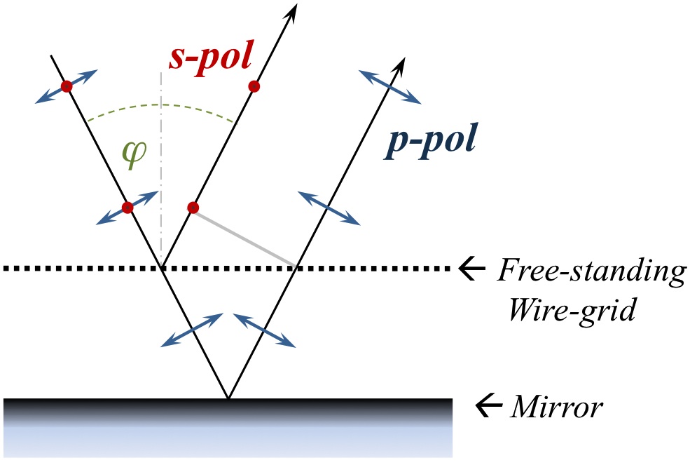
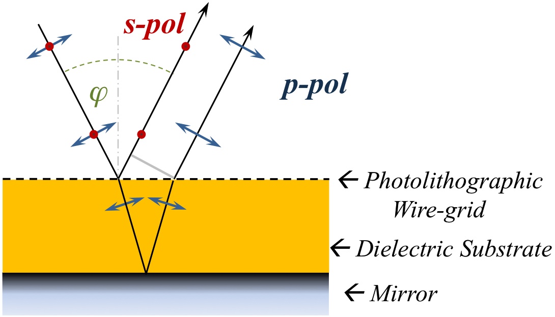
Figure 27: Left: Free-standing RHWP. Right: Dielectric substrate RHWP

The absorption is due to the power dissipated in the metal and along the wires. For a flat metal absorption for the ‘s’ and ‘p’ polarizations are always slightly different, the latter being lossier. The losses increase with frequency but can be reduced by decreasing the device temperature. For a copper RHWP at 30 K used at $\phi=45^{\circ}$ incidence and assuming an ideal wire-grid, the differential absorption coefficient between for the ‘s’ and ‘p’ polarizations is of order 10^-4. However, while the RHWP is rotating, the s and p absorption coefficients fluctuate at a frequency 2$\omega$ with averaged fluctuation amplitudes of 6$\times 10^{-5}$ and 1.5$\times 10^{-5},$ respectively.

A dielectric substrate RHWP fabricated using photolithographic techniques could be used to solve the free-standing RHWP manufacturing problems. The air gap between the wire grid and the mirror is replaced by a dielectric substrate and the the wire grid is directly imprinted on one of the substrate surfaces (Fig. 27). The presence of the dielectric substrate introduces frequency-dependent standing waves (multiple reflections). Their amplitude depends on the type of polarization ‘s’ or ‘p’ passing through. Models show that modulation efficiency deteriorates with increasing substrate refractive index. For a substrate with $n=1.2,$ the efficiency drops to  0.4, which can be improved through spectral filtering. However, the absorption value then changes slightly with the RHWP orientation. These additional losses due to resonances appear at frequencies corresponding to the modulation efficiency peaks. For a RHWP at 30 K made out of copper, the values are within the following ranges: $A_{s}=1.3-1.8\times 10^{-4}$, $A_{p}=2.6-2.7\times 10^{-4}$. (This means that the ‘s’ and ‘p’ components of an unpolarized background signal is modulated at 2$\omega$ with relative amplitudes of $5\times 10^{-5}$ and $10^{-5}$ respectively). While presently rated only at TRL 4, we are choosing the dielectric substrate RHWP as the modulator baseline for COrE as it offers the best potential performances and manufacturability. Indeed it is modelled on the dielectric embedded interference filter technology flown on PLANCK and Herschel.

Manufacturing the free standing RHWP is challenging because required diameter exceeds 1 meter. The mechanical structure of the free-standing wire-grid must guarantee a constant spacing between the wires and a constant distance from the mirror across the entire surface. To our knowledge, the biggest device of this type ever built has a diameter of 0.5 m [286].

Commercially available dielectric laminates used in microwave engineering to build planar microstrip circuits could be used to build a dielectric substrate RHWP. These laminates come in different sizes, thicknesses, and refractive indices, and have copper deposited on both sides. One possibility is to use one metallic side as a mirror and photolithographically etch the other side of the substrate in order to produce metallic stripes in the place of a wire grid. The resolution required for the mask production in our frequency range is achievable with large commercial printers. The laminate can be joined to a thick metallic flat surface to increase the structure stiffness. Note that the main problems of the free-standing RHWP would thus be resolved. The constant spacing between wires is guaranteed by the high accuracy of the photolithographic techniques whereas the constant distance between the mirror and wire elements comes directly from the accurate constant thickness of the laminates required in microstrip circuits.

Polarization modulator rotation mechanism

The RHWP needs to be rotated. While a step and integrate rotation could be considered, a continuous rotation at 0.1 to a few rpm is preferable both for the observation strategy (§ 5.2) and to avoid disturbing the rotation of the satellite. Such a strategy has been adopted on the Maxima and EBEX balloon-borne experiments for which a superconducting magnetic bearing has been developed. The HWP rotates at 2 Hz with low frictional dissipation. This is a crucial parameter as the RHWP will have to operate at the lowest temperature possible (30K here) in order to reduce the systematic effects arising from thermal emissivity.

The rotation will be driven by a motor operated at a higher temperature within the service module where a larger cooling power is available (shown in Fig.21). The difficulty resides in having to rotate a HWP of 1.7 m diameter, weighting approximatively 25 kg including its support structure kept at 30 K. The technology is rated TRL 8, the associated risks being the mass and dissipated power.

The main problems associated with this subsystem are thermal and mechanical. The thermal dissipation of the bearings, thermal conduction through the shaft, and microphonic vibrations possibly coupling to the detectors are areas of concern.

Shaft:

For transmitting the torque from the motor (located in the service module) to the RHWP, a long fiberglass shaft is a good solution but this option needs further development. The critical points are related to the thermal and dynamical aspects of the shaft. It will have to operate at low temperature (down to 35 K), be a good insulator, resist launch and should not create vibrations while rotating. The effect of the differing thermal expansion coefficients at the interface between this composite material and the metal needs to be studied more carefully.

The shaft diameter will be studied with the stress criteria (torque transmission) and the dynamic criteria (modes for launch and no torsional modes to not interfere with the motor) potentially leading to higher thermal conduction between the temperature stage of the motor and the 30 K of the RHWP. If so, magnetic contact-less coupling devices could be investigated in order to reduce the thermo-mechanical aspects of the shaft.

Bearings:

Conventional bearing mechanisms for the RHWP will need to be studied for lubrications problems when operated at 30 K. A dry lubrication solution might be adopted. However, in order to decrease the thermal dissipation, a high temperature superconducting magnetic bearing, such as the one developed for EBEX [287], would be a better solution completely avoiding the problem of lubrication, but this option requires further development. Moreover, it has to be noted that NASA for instance is designing successfully flywheels for spacecrafts based on magnetic bearings. With a top speed of 40,000 rpm and a potential lifetime of 20 years the requirements are largely above ours. This is a parallel research on which we could also base our design for a superconductive magnetic bearing.

5.3.3 Detectors and readout electronics

In the frequency range of COrE, bolometers cooled to very low temperature ($T\leq 100$mK) currently offer the best performances for broad bandwidth detection. With a careful instrument design, their sensitivity can approach the photon shot noise of the astrophysical source. The understanding of bolometer performance in a space environment has dramatically advanced as a result of the PLANCK mission. In order to read out the large number of detectors required, transition edge superconducting bolometers (TESs) are used. Various materials can be combined to form the thermal sensor. Thin films such as NbSi or bilayer like MoCu are possible. The critical temperature of these sensors has to be matched to the power handling and cooling requirements of the instrument. TESs have been developed extensively for astronomical observations from millimeter through X-ray wavelengths and have a long history of use.

Microstrip-coupled TES technology is the detector baseline for COrE, where thin-film waveguide antennas in the OMT are used to couple radiation from a horn antenna onto the TES through a superconducting microstrip transmission line terminated with a resistor. The detector would be located on the same wafer as the OMTs using microfabrication techniques demonstrated for superconducting bolometer arrays for ground based experiments like QUBIC, SCUBA2, or Clover.

Detailed models (assuming 50% optical efficiency, a 30 K telescope with 1% emissivity, and 15 GHz bandwidth) predict a photon NEP of about $4\times 10^{-18}W~{}Hz^{-1/2}$ in all wavebands except for the last 3 bands which have a larger bandwidth of 195 GHz. A sensitivity requirement for the detectors has been chosen at 70% of the photon noise or $3\times 10^{-18}W~{}Hz^{-1/2}$ which increases the total NEP by about 22%. More details are given in table 8.

In June 2010, absorber-coupled TESs were down-selected by an international panel for the FIR imaging arrays on the SAFARI instrument on the cooled-aperture telescope on SPICA. A European consortium now routinely makes and measures MoCu, MoAu, and TiAu TES arrays having thermal conductances of 0.2 pW/K, and NEPs of $5\times 10^{-19}W.Hz^{-0.5}$. A substantial amount of work is currently taking place in the context of developing space qualifiable, ultra-low-noise, SQUID multiplexed, TES arrays for SAFARI, and this work will be of substantial benefit to COrE. COrE requires microstrip-coupled TESs having differential thermal conductances of typically 10 pW/K, and NEPs of typically $<5\times 10^{-18}W.Hz^{-0.5}$, which is an order of magnitude less demanding than SAFARI. By combining the microstrip-coupled TES technology developed several years ago for ground-based astronomy, having NEPs $<5\times 10^{-17}W.Hz^{-0.5}$ (Fig 28-right), together with the state-of-the-art absorber-coupled TES technology being developed for SAFARI having NEPs $<5\times 10^{-19}W.Hz^{-0.5}$, we can produce TES detectors having the needed specifications for COrE. The time constant of the detectors should be shorter than the time needed to scan a beam in order not to degrade the angular resolution. The stringent constraint is therefore given by the high frequency channels where the beam size is smallest. Under the proposed design, the required time constant ranges from 10 ms to 0.6 ms. TESs operate through a strong electro-thermal feedback mechanism, which speeds up their effective time response to the sub-ms values required by COrE. Once again, the work on SAFARI has shown that achieving the time constants needed for COrE is straightforward. Overall, the main technological challenges will be associated with realizing the extremely large array, rather than any fundamental problems associated with producing individual pixels having the needed performance.

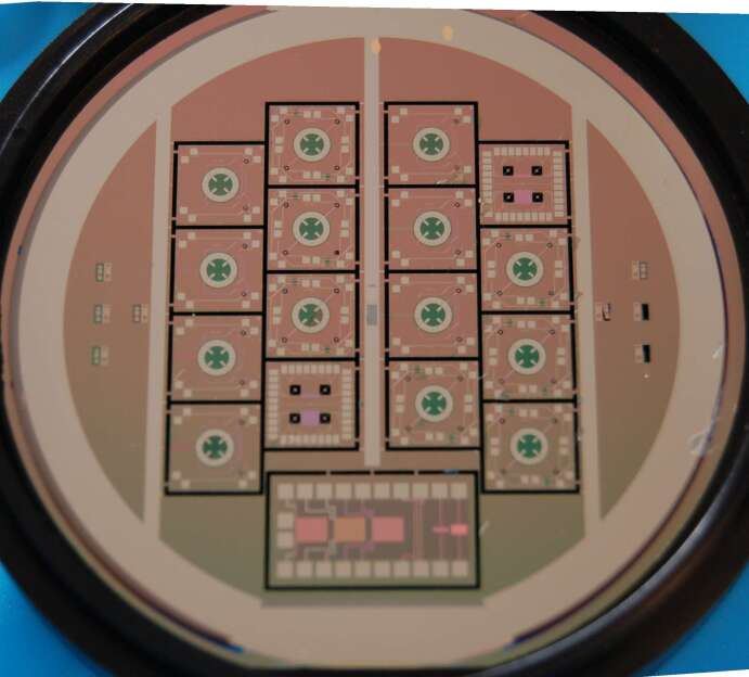
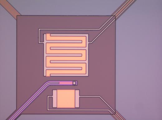
Figure 28: Left: A wafer of polarization sensitive MoCu TESs. The 4, thin-film, SiN membrane suspended waveguide probes can be seen (Cambridge Univ.). Right: A microstrip-coupled MoCu TES suitable for ground-based polarimetry (Cambridge Univ.).

The readout system of bolometer arrays requires multiplexing to decrease the thermal load on the final cryogenic stage and also to simplify the architecture. The COrE design uses time domain multiplexing with SQUIDs as the first amplifier stage. A standard SiGe BiCMOS ASIC (Application Specific Integrated Circuit) cooled to 80K is used to control the multiplexing sequence and to amplify the signal from the SQUIDs. This technology has been tested in space by NASA during the MISSE-6 mission aboard the ISS. A multiplexing factor of 24 has been demonstrated with a heat load of 20 mW down to 4 K. Assuming the same power dissipation, we have finalized a new design to readout 128 detectors with one ASIC. The COrE architecture requires 50 of these new ASICs, leading to a power load of about 1 W. Further improvement in power dissipation and multiplexing factor is anticipated during the phase A study.

We are also considering using superconducting microwave kinetic inductance detectors (MKIDs). These are new devices operating at 0.1K promising high-sensitivity large-format detector arrays. The MKIDs concept was proposed in 2002 [283]. In an MKID low energy photons (in the meV range) break Cooper pairs in a superconducting film, thus changing its surface impedance and in particular its kinetic inductance. The detector consists of a superconducting thin-film microwave resonator capacitively coupled to a probe transmission line. This is typically a quarter-wavelength of coplanar waveguide (CPW), capacitively coupled to a feedline (i.e., a distributed resonator). By exciting the electrical resonance with a microwave probe signal, the transmission phase of the resonator can be monitored, allowing the deposition of energy or power to be detected. The KIDs read each pixel at a separate frequency. Therefore only one pair of coaxial leads is needed to connect several thousand pixels to the readout electronics thus simplifying the thermal architecture. An example of some of these developments is shown in Fig. 29. A different approach has been proposed [284] in which a lumped RLC series resonant circuit is inductively coupled to the feedline (LEKID). These devices have been demonstrated in a laboratory environment and have already been implemented in various demonstrator instruments in the millimeter and submillimeter bands [285].

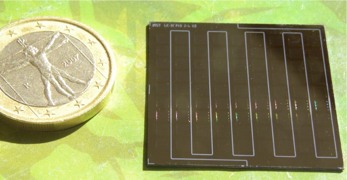
Figure 29: An 81-pixels array of kinetic inductance detectors for the 140 GHz band, developed in Italy under the RIC program of INFN and the ACDC program of PNRA [276].

Cold electron bolometers are a third technology option worth mentioning. These detectors developed in Sweden (Chalmers) are starting to give promising laboratory results [288].

Over the last few years many national funding agencies have invested heavily in establishing superconducting detector fabrication facilities in Europe. Major facilities exist in the UK, France, the Netherlands, Sweden, Germany, and Italy. These facilities not only provide clean rooms with lithography, processing, and test equipment, but also provide professional, traceable fabrication routes, producing high-quality high-yield devices. A major part of the technology development, fabrication, and test program will be to form a single network coordinated by one lead organization, with all of the partner organizations working towards the refinement of a single design across all of the chosen wavebands. Most of these laboratories are working on the development of TESs and KIDs as shown in Table 7.

Table 7: List of different detectors technologies which could be adapted to COrE specifications.

Technology	Partnership	Achievements	Papers
Single and dual	UK: Cambridge and Cardiff	ClOVER, and study for a COrE	[292]-[296]
polarization TESs		type mission - ESA TRP contract.
with feedhorns	US: NIST and GSFC		[297]
and waveguide	It - ASI technology contract		[298]-[301]
probes coupled	Fr: APC, CSNSM, IAS	NbSi bolometers
to microstrip	IEF, Institut Néel, IRAP	with low temperature SiGe	[302]-[306]
transmission lines	L2E, LERMA, LPSC	ASIC for TDM readout
TES detectors with	US	Detectors assembled	[307]
feedhorns & distributed		in a large array (966 pixels)
absorber (unpolarized)		Scientific breakthroughs at the SPT
Planar antenna coupled	US: UC Berkeley	POLARBEAR	[308]
TESs - dual polarization		EBEX balloon experiment	[309]
broadband + multifreq.		TRL=6 with about 1300 detectors
capability - lens-coupled
Planar antenna coupled	US: JPL	BICEP and the Keck Array
TESs with planar phased		(2048 bolometers) at the South Pole
array antennas		balloon-borne experiment SPIDER	[310]
dual polarization		Close to 99% yield	[311]
single frequency
Free space coupled	Fr: LETI- CEA	Herschel-PACS: Array of 2560 pixels	[312] [313]
detectors single or	& CEA-DSM-DAPNIA	$NEP=1.5.10^{-16}$, BW=5Hz
dual polarization		can be improved for the high
absorbers		frequency bands of COrE
LEKID/KID arrays	UK, It, NL, Fr, Sp	camera (2x112 pixels) at IRAM 30m	[314] [314]
		81 pixels array made in Italy-Fig 29	[276] [316]

5.3.4 Spectral filtering

Because bolometric detectors are sensitive to a broad spectral range, their spectral band definition requires special attention. COrE requires a high in-band transmission in order to reach a 50% overall optical efficiency while rejection of optical/NIR power must be better than $\approx 10^{-12}$ although a rejection of $\approx 10^{-6}$ suffices in the FIR. Low frequency rejection is easily achieved through the horn waveguide design. The PLANCK-HFI-like high frequency band definition based on dielectric embedded interference filters requires several multilayer mesh filters in series located on the different temperature stages also limiting the thermal power reaching the ultra-cold stages. This technology, selected as the baseline for COrE, allows for use with mixed frequency array by arranging their geometry to suit the shape of the sub-array. It is also conceivable to make a unique filter made of several regions. However special attention is required to avoid straylight in between the different regions of this filter potentially leading to cross-talk between channels.

In order to reduce the number of interference filters mentioned above, superconducting planar bandpass filters could be lithographed onto the detector chips, which together with a planar OMT would lead to intrinsic on-chip polarimetry. While parts of this technique has been demonstrated, further development is necessary.

Additional spectral filtering: As mentioned in § 5.3.2, the modulation efficiency of the high frequency channels can be increased using broader bands in combination with sub-band selective filtering around the peaks. This can be achieved for example by using multilayer dielectrics that act as dielectric mirrors. However, while the RHWP modulation efficiency peaks are centered at an odd multiple number of its basic frequency as shown in eqn. 24, the filter transmission bands are centered at an even multiple number of its basic frequency following eqn. 25. So a slightly different basic frequency $\nu_{0}^{Filter}$ will be used for the filter so that we have maximum coincidence between the two sets of peaks. The example in Fig. 30 shows a candidate filter around the 795 GHz peak using $\nu_{0}^{Filter}=15.29$ and $n=26$.

$$\nu_{n}^{Filter}=2n\times\nu_{0}^{Filter}$$ (25)

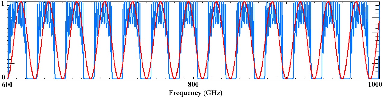
Figure 30: Sub-band filtering: Filter transmission (blue) and RHWP efficiency (red).

5.3.5 Cryogenic chain

Since the mass and power requirements and the temperature stages are similar to those of PLANCK, copying the PLANCK cryogenic chain would bring the whole system to TRL 9. However several modification would provide superior performance. The main objective is to develop a system based on mechanical coolers and recyclable system to provide for a long duration mission. Below is a summary of a CNES study.

Passive cooling:

The V-grooves used in PLANCK to radiate power into free space placed laterally to the spin axis have proven to be an efficient solution to a first passive cooling stage. They also provide cooling to intermediate stage electronics. An inner V-groove temperature of 50 K is currently achieved in orbit with an available power of the order of 1 W for PLANCK. With further optimization and the addition of a fourth V-groove, a temperature of about 35 K could be achieved for COrE inner V-groove.

Active cooling - Mechanical coolers

The 35K to 20K

stage could be provided by a H₂ JT (Joule-Thomson) cooler with metal-sorption compressor from JPL (PLANCK). However a pulse tube cooler (PTC) providing 15/20 K stage is under development at Air Liquide/CEA (with the goal to reach 15K). Note that a two-stage PTC with a 300 mW heat lift at 20 K (with intercept) has already been demonstrated on the GSTP program 20-50K Pulse Tube (ESA contract 20497/06/NL/PA). Ongoing developments will allow more margin at the 20K stage. This 20 K PTC stage requires a pre-cooling at 80 K with a heat intercept cooling power of about 6 W. Note that pre-cooling at a higher temperature (e.g., 120 K) is possible but with a slight decrease of the performance at 20 K. This heat intercept can be provided either by a V-groove through thermal braids links for example (preferred solution), or by a dedicated 80 K PTC. Maturity level of the 20 K PTC is considered TRL 4.
The 15 K to 4 K stage is provided by a Joule-Thomson (JT) cooler similar to the PLANCK cooler.

Active cooling - Sub-K coolers:

Because the open cycle dilution refrigerator (OCDR) providing both the 1.7 K and 100 mK stages from 4 K on PLANCK has a limited lifetime, a recyclable system is preferable. The 0.1 K stage baseline could be provided by an ADR cryocooler (e.g. from CEA SBT), requiring pre-cooling (e.g., at 1.7K and 4K on SAFARI/SPICA) or a continuous ADR 4-stage (NASA-GSFC) developed for MIRI (JWST). While ADRs are already at TRL 9 (XRS on ASTRO-E2), the strong associated magnetic field might affect the operation of the TES readout system (SQUIDs), although efforts are being dedicated to mitigate this difficulty.

For this reason, a closed cycle dilution refrigerator (CCDR) based on the heritage of the flight-proven OCDR can offer a more convenient solution. The re-circulation of the helium isotopes (He-3 and He-4) of this system allows for no theoretical limitation on lifetime. Contrary to the OCDR, the CCDR requires a pre-cooling stage around 1.7 K in order to evacuate the heat from thermalization of He-3 and He-4 gas flows and from condensation of He-3 (a fraction this heat is used for the evaporation of He-3 but not all of it). It is not possible to produce a 1.7 K stage with a He-3 Joule-Thomson expansion within this dilution system. As a consequence, the 1.7 K stage is produced by a dedicated He-4 sorption cooler based on the concept of the Herschel He-3 sorption cooler. The CCDR system also provides extra cooling power between 200 mK and 600 mK if needed (e.g. for thermalization of mechanical supports or harnesses). The maturity level of CCDR is considered TRL 4, and should reach TRL 5 within 2 years with ongoing developments at Air Liquide/CNRS Neel institute.

5.3.6 Data Rate

Every day the instrument will simply survey the sky for 24 hours according to the predefined program with a sampling rate matching the scan speed of 0.5 rpm and the FWHM of the beam for each frequency channel. Based on Planck experience, we request 16 bits per scientific data sample and 5 samples per beam. Taking into account a compression factor of 4, we reduce the resulting total raw data rate of 18 Mpbs (see Table 8) to 4.5 Mbps for transmission.

The on-board data storage system should be able to save a few days of data ( i.e. $4.5\times 10^{6}\times 86400\times 2$ = 780 Gbit, instead of the 32 Gbit memory on board of Planck) in order to cope with downlink problems due to contingencies in the telecommunication system. The data will be dumped to the Earth via a high-gain antenna aligned to the spin axis for about 2 hours per day in the Ka band, during which the spin axis will be directed to the Earth. In this case we shall need a data dump rate of $4.5\times 12$ = 54 Mbit/s.

5.4 Expected performance

The sensitivity of a perfect instrument with a uniform coverage of the celestial sphere, expressed in terms of noise angular amplitude spectrum $c_{noise}$, is given by eqn. 26 assuming a polarization modulation efficiency of 80%, where $t_{miss}$ is the total mission duration, $N_{det}$ is the number of detectors and $s_{det}$ is the sensitivity in intensity of one detector

$$c^{2}_{noise}=2.4\times\frac{4\pi}{t_{miss}N_{det}}\times s^{2}_{det}=\left(4.7\mu K\cdot arcmin\right)^{2}\times\left(\frac{4~{}years}{t_{miss}}\right)\times\left(\frac{400}{N_{det}}\right)\times\left(\frac{s_{det}}{50\mu K\cdot s^{\frac{1}{2}}}\right)^{2}.$$ (26)

To reach such sensitivity, the proposed instrument architecture is designed in order to have background limited performances. The detector number is furthermore optimized to reach the required sensitivity in each channel and to fill the focal plane area. With the current instrument design, this process leads to the numbers given in Table 1. The proposed configuration has a total of 6384 detectors in 15 frequency bands. The greatest sensitivity is concentrated in the CMB channels (75GHz-225GHz) with 4950 detectors.

Table 8: COrE detector specifications with assumptions from § 5.3.3 for NEPs calculations. Data rates based on § 5.3.6 assumptions give a total of 18 Mbit/s.

Central Freq.	$NEP_{phot}$	$NEP_{det}$	$NEP_{tot}$	Data rate / waveband	Det. time constant
(GHz)	$(W.Hz^{-0.5})$	$(W.Hz^{-0.5})$	$(W.Hz^{-0.5})$	(kbit/s)	(ms)
45	$4.4\times 10^{-18}$	$3.1\times 10^{-18}$	$5.4\times 10^{-18}$	38	10.7
75	$4.5\times 10^{-18}$	$3.2\times 10^{-18}$	$5.5\times 10^{-18}$	298	6.4
105	$4.4\times 10^{-18}$	$3.1\times 10^{-18}$	$5.4\times 10^{-18}$	557	4.6
135	$4.3\times 10^{-18}$	$3.0\times 10^{-18}$	$5.3\times 10^{-18}$	985	3.6
165	$4.1\times 10^{-18}$	$2.9\times 10^{-18}$	$5.1\times 10^{-18}$	1642	2.9
195	$4.0\times 10^{-18}$	$2.8\times 10^{-18}$	$4.8\times 10^{-18}$	2975	2.5
225	$3.8\times 10^{-18}$	$2.7\times 10^{-18}$	$4.7\times 10^{-18}$	5373	2.1
255	$3.7\times 10^{-18}$	$2.6\times 10^{-18}$	$4.5\times 10^{-18}$	1945	1.9
285	$3.6\times 10^{-18}$	$2.5\times 10^{-18}$	$4.4\times 10^{-18}$	1418	1.7
315	$3.6\times 10^{-18}$	$2.5\times 10^{-18}$	$4.4\times 10^{-18}$	418	1.5
375	$3.6\times 10^{-18}$	$2.5\times 10^{-18}$	$4.4\times 10^{-18}$	318	1.3
435	$3.6\times 10^{-18}$	$2.5\times 10^{-18}$	$4.4\times 10^{-18}$	369	1.1
555	$13.7\times 10^{-18}$	$9.7\times 10^{-18}$	$1.7\times 10^{-17}$	471	0.9
675	$14.2\times 10^{-18}$	$1.0\times 10^{-17}$	$1.7\times 10^{-17}$	573	0.7
795	$14.5\times 10^{-18}$	$1.0\times 10^{-17}$	$1.8\times 10^{-17}$	675	0.6

5.4.1 Configuration evolution

Tables 1 and 8 give the present configuration. However in order to increase significantly the sensitivity at high frequency and strengthen the galactic science output, an option under study is to increase the number of detectors of the 795 GHz spectral band by a factor 5. As shown in figure 22 this will have little impact on the overall focal plane dimension (all 64 detectors - 32 pixels - are represented by the red circle at the center of the FPU). While the sensitivity of this band will be increased by a factor $\sqrt{5}$, the total data rate will increase by 15%.

5.5 Calibration

To keep the instrument simple and without a possible single point failure, no onboard calibration system is included. COrE calibration will rely on ground calibration sequences and astrophysical sources that will have been thoroughly studied by PLANCK and follow-up observations. Systematic effects affecting the polarization purity of the incoming signal will be mitigated by the RHWP in front of the telescope. However the RHWP might introduce small beam shape distortions synchronous with its orientation that should be detected and characterized in the calibration process to ensure a negligible impact on the measurements. The ground calibration will consist of the following complementary tests:

Sub-system level: (detectors, reflective optics, cold optics, RHWP, cooling system)

FPU: spectral response of each pixel, dark and illuminated I-V curves for various FPU temperatures.

Warm RF test in Compact Antenna Test Range: RF test conducted during the PLANCK ground calibration campaigns have been extremely beneficial in order to characterize the main and far-side lobes of the telescope beams. RF performance have been measured with a few representative horns associated with OMTs and warm detectors (heterodyne instead of bolometers) in conjunction with the telescope and the shields. Similar test including the RHWP will be performed in order to measure and model the systematic effects introduced by the RHWP. Such effects are already under study at pixel level. Several CMB polarization experiment are making use of a half-wave plate. Most of these are using birefringent HWP located in front of the focal plane, at the entrance aperture of the horns. Figure 31 is showing such a measurement taken in the frame of the Clover project. It shows the variation of the beam shape that can be expected when a birefringent HWP is rotated in front of a horn. In this instance the impact is minimal down to -25 dB and the cross-polarization integrated over the horn main beam remains below -35 dB. Preliminary studies are being carried out in the framework of R&D programs with higher precision measurements allowing to develop and validate theoretical models predicting such systematic effects. Similar measurements on the effects of a RHWP in front of a telescope like COrE could be performed in the framework of a M3 mission.

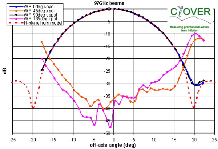
Figure 31: Systematic effect caused by a birefringent HWP on a corrugated horn beam. Measurements performed with a vector network analyzer (75-110GHz) at the University of Manchester for the Clover project. The red dashed line is the predicted horn co-polarization beam, the solid lines the beams with different orientations of the HWP in front of the horn aperture.

Dedicated calibration facility reproducing the cryogenic and radiative environment expected during the mission is envisaged. A large vacuum chamber fitted with a 2K cryogenic chain and a full beam source will be prepared. The chamber will allow operation of the entire instrument, observing a 2.7 K load and a polarized source modulated and oriented as needed. This setup will allow the precise determination of the polarimetric parameters of the instrument (polarization efficiency and main axis angles) and of the responsivity and noise of all the detectors for different radiative loading conditions. The proposers inherit considerable experience from similar calibration facilities built for Archeops and BOOMERanG as well as from the calibration campaign on PLANCK at CSL-Liège.

6 Epilogue

The COrE proposal was submitted to ESA on 13 December 2010 in response to a call for an M3 ‘medium-sized’ space mission in the framework of Cosmic Vision 2015-2025. The COrE collaboration includes the European CMB community (a full list of endorsers can be found on the website www.core-mission.org) and the US CMB community has expressed a strong interest in a NASA participation should the ESA proposal be successful. ESA is currently in the process of evaluating the COrE proposal.

Compared to the previous B-Pol proposal submitted to ESA three years ago, COrE has a higher angular resolution and broader frequency coverage, allowing COrE to broaden its science program substantially. Roughly speaking the size of the instrument is more or less fixed, being determined by the budget and physical dimensions of the launch vehicle. While B-Pol proposed several refractive telescopes, each tailored to a particular frequency range, and relied on a complex scan strategy to control systematic effects, COrE will have a single reflective telescope, suitable over the entire frequency range, and use a rotating reflective half-wave plate as the first optical element in front of the sky to modulate away most of the parasitic systematics. It is this feature that makes COrE unique and allows numerous requirements to be relaxed relative to what would be needed in the absence of such modulation. The enhanced resolution of COrE, owing to the large size of the mirror, is diffraction limited at all frequencies, unlike PLANCK, reaching a resolution of 1.3 arcmin in the highest 795 GHz channel. In the CMB channels the resolution ranges from 10 arcmin (105 GHz) to 4.7 arcmin (225 GHz) and the polarization sensitivity (for a four-year mission) is around $4.5\,\mu\mathrm{K}\,\mathrm{arcmin}$.

The broad frequency coverage in 15 narrow bands, and the high sensitivity, will allow reliable subtraction of foregrounds in the search for primordial B modes due to the gravitational wave background from inflation. Our simulations indicate that a tensor-to-scalar ratio $r=10^{-3}$ should be detectable at $3\sigma$, corresponding to an energy scale of inflation (few)$\times 10^{15}$ GeV. The high resolution in the CMB channels will allow COrE to carry out virtually the ultimate CMB lensing experiment, with the deflection field reconstructed with high signal-to-noise on all scales where linear theory is reliable. In addition, COrE will have great discovery potential in the area of non-Gaussianity being able to search for a variety of “shapes” of the primordial $n$-point functions. This ability to fingerprint the physics of inflation sets the CMB apart from other probes of non-Gaussianity. COrE will also be able to do breakthrough galactic and extragalactic science in the far infrared, mapping the dust polarization at high resolution in the regions of diffuse emission, and hence map the galactic magnetic field, thus answering key questions concerning the mechanisms of star formation. Thanks to its exquisite resolution and sensitivity, COrE will also discover a myriad of new IR compact sources, both polarized and unpolarized. At the other end of the spectrum, at low frequencies COrE will be 30 times more sensitive than PLANCK LFI, providing exquisite maps of the galactic synchrotron emission free of Faraday rotation.

7 Selected references

We provide here an abridged set of essential references concerning the polarization, CMB, and sub-millimeter science and instrumentation.

The COrE team has benefited from experience in a variety of suborbital and space CMB experiments, including most notably Boomerang, CLOVER, and PLANCK (http://www.esa.int/SPECIALS/Planck/index.html). We have also benefited from several B-mode polarization satellite studies starting with the Frech CNES-sponsored SAMPAN study and the Italian COFIS study of ASI, leading to European B-Pol proposal three years ago. (www.b-pol.org) A more detailed American CMBPol study followed on this heritage, producing a number of useful and detailed white papers, which broadly confirm the conclusions of the present study. In particular, the following papers provide useful details and extensive references:

J Dunkley et al., “CMBPol Mission Concept Study: Prospects for polarized foreground removal,” (arXiv:0811.3915[astro-ph]) (2008)

A Fraisse et al., “CMBPol Mission Concept Study: Foreground Science Knowledge and Prospects,” (arXiv:0811.3920[astro-ph]) (2008)

D Baumann et al., “CMBPol Mission Concept Study: Probing Inflation with CMB Polarization,” (arXiv:0811.3919[astro-ph]) (2008)

M Zaldarriaga et al., “CMBPol Mission Concept Study: Reionization Science with the Cosmic Microwave Background,” (arXiv:0811.3918[astro-ph]) (2008)

K Smith et al., “CMBPol Mission Concept Study: Gravitational Lensing,” (arXiv:0811.3916[astro-ph]) (2008)

More information is at http://cmbpol.uchicago.edu/. We following publications are particularly relevant:

Reichborn-Kjennerud B. et al., “EBEX: A balloon-borne CMB polarization experiment,” Proceedings of the SPIE, Volume 7741, pp. 77411C-77411C-12 (2010) (arXiv:1007.3672)

D Chuss, “Quasioptical Reflective Polarization Modulation for the Beyond Einstein Inflation Probe” in Polarization Modulators for CMBPol, J of Phys: Conf. Series 155 (2009).

L Verde, H Peiris & R Jimenez, “Optimizing CMB polarization experiments to constrain inflationary physics,” JCAP 0601, 019 (2006) (astro-ph/0506036)

de Zotti, G., et al., “Radio and millimeter continuum surveys and their astrophysical implications”, (A&ARv 18, 1) (2010).

Lagache, G., et al., “Dusty Infrared Galaxies: Sources of the Cosmic Infrared Background”, (ARA&A Annual 43, 727) (2005)

J Fergusson, M Liguori, P Shellard, “General CMB and Primordial Bispectrum Estimation I: Mode Expansion, Map-Making and Measures of $f_{NL},$” Phys. Rev.D82, 023502 (2010) (0912.5516/astro-ph.CO)

A Lewis & A Challinor, “Weak gravitational lensing of the CMB,” Phys. Rept. 429, 1 (2006) (astro-ph/0601594)

C McKee & E Ostriker, “Theory of Star Formation,” ARAA 45, 565 (2007)

J Delabrouille & J Cardoso, “Diffuse Source Separation in CMB Observations,” (astro-ph/0702198)

S Leach et al., “Component separation methods for the PLANCK mission,” A& A 491, 597 (2008) (arXiv:0805.0269)

A more detailed bibliography arranged section by section appears on the COrE website cited above.

References

- [1]
- [2]
- [3] Starobinsky A. A., Sov. Astron. Lett. 11, 133 (1985).
- [4] Linde A. D., Phys. Lett. B129, 177 (1983).
- [5] Barrow J. D., Phys. Lett. B235, 40 (1990).
- [6] Silverstein E. and Westphal A., Phys. Rev. D. 78, 106003 (2008).
- [7] Linde A. D., Phys. Lett. B108, 389 (1982).
- [8] Albrecht A. and Steinhardt P. J., Phys. Rev. Lett. 48, 1220 (1982).
- [9] Freese K., Frieman J. A. and Olinto A. V., Phys. Rev. Lett. 65, 3233 (1990).
- [10] Linde A. D., Phys. Lett. D. 49, 748 (1994).
- [11] Liddle A. R., Mazumdar A. and Schunck, F. Phys. Lett. D. 58, 061301 (1998).
- [12] Dimopoulos S., Kachru S., McGreevy J. and Wacker J. G., JCAP 08, 003 (2008).
- [13] Linde A. D. and Mukhanov V., Phys. Rev. D. 56, 535 (1997).
- [14] Lyth D. H. and Wands D., Phys. Lett. B 524, 5 (2002).
- [15] Dvali G. and Tye S.-H. H, Phys. Lett. B 450, 72 (1999).
- [16] Kachru S., Kallosh R., Linde A. D., Maldacena J., McAllister L. and Trivedi S. P., JCAP 10, 013 (2003).
- [17] Baumann, D., et al. 2009, APS Phys. Conf. Series 1141, 10, arXiv:0811.3919
- [18] Easther R., Kinney W. H., 2003, Phys. Rev. D 67, 043511
- [19] Efstathiou G., Mack K. J., 2005, JCAP 0505, 008, astro-ph/0503360
- [20] Hoffman M. B., Turner M. S., 2001, Phys. Rev. D 64, 023506
- [21] Kinney W. H., 2002, Phys. Rev. D 66, 083508
- [22] Kinney W. H., 2003, New Astron. Rev. 47, 967
- [23] Kinney W. H., Kolb E. W., Melchiorri A., Riotto A., 2004, Phys. Rev. D 69, 103516
- [24] Knox L., Song Y., 2002, Phys. Rev. Lett. 89, 011303
- [25] Liddle, A. R. 2003, Phys. Rev. D 68, 103504
- [26] Lyth D. H., 1984, Phys. Lett. B, 147, 403
- [27] Lyth D. H., 1997, Phys. Rev. Lett. 78, 1861
- [28] Peiris H. V., Komatsu E., Verde L., Spergel D. N., Bennett C. L., Halpern M., Hinshaw G., Jarosik N., Kogut A., Limon M., Meyer S. S., Page L., Tucker G. S., Wollack E., Wright E. L., 2003, ApJS, 148, 213
- [29] Chongchitnan S. and Efstathiou G., Phys. Rev. D. 72, 083520 (2005).
- [30] Verde L., Peiris H. V., Jimenez R., 2005, JCAP, 1, 19
- [31] Fisher R. A., 1935, J. Roy. Stat. Soc., 98, 39
- [32] Smith, K. M. et al., “CMBPol Mission Concept Study: Gravitational Lensing,” (2008) (arXiv/0811.3916)
- [33] Perotto, L., Lesgourgues, J., Hannestad, S., Tu, H., & Wong, Y., ”Probing cosmological parameters with the CMB: forecasts from Monte Carlo simulations,” JCAP 10, 13 (2006) (arXiv:astro-ph/0606227)
- [34] Hannestad, S., ”Neutrino physics from precision cosmology,” Prog. in Part. and Nucl. Phys. 65, 185 (2010) (arXiv/1007.0658)
- [35] LSST Science Collaborations and Abell, P. A., Allison, J. Anderson, S. F. Andrew, J. R. Angel, J. R. P. Armus, L. Arnett, D. Asztalos, S. J. Axelrod, T. S. et al., ”LSST Science Book, Version 2.0,” (2009) (arXiv/0912.0201)
- [36] Hu, W. and Okamoto, T., ”Mass Reconstruction with Cosmic Microwave Background Polarization”, Ap. J. 574, 566 (2002) (arXiv:astro-ph/0111606)
- [37] Calabrese, E., de Putter, R., Huterer, D., Linder, E. V., and Melchiorri, A., ”Future CMB Constraints on Early, Cold, or Stressed Dark Energy,” (2010) (arXiv/1010.5612)
- [38] Smith, K. M.; Zahn, O.; and Doré, O., ”Detection of gravitational lensing in the cosmic microwave background,” Phys. Rev. D76, 043510, (2007) (arXiv/0705.3980)
- [39] Nakamura, K. et al., ”The Review of Particle Physics”, J. Phys. G 075021 (2010)
- [40] Refregier, A. Amara, A. Kitching, T. D. Rassat, A. Scaramella, R. Weller, J. and Euclid Imaging Consortium, “Euclid Imaging Consortium Science Book,” (2010) (astro-ph/1001.0061)
- [41] Lewis, A. and Challinor, A., ”Weak gravitational lensing of the CMB,” Phys. Reps. 429,1 (2006) (arXiv:astro-ph/0601594)
- [42] R. Jeannerot, J. Rocher and M. Sakellariadou, “How generic is cosmic string formation in SUSY GUTs,” Phys. Rev. D 68, 103514 (2003) [arXiv:hep-ph/0308134].
- [43] A. D. Linde, “Hybrid inflation,” Phys. Rev. D 49, 748 (1994) [arXiv:astro-ph/9307002].
- [44] E. J. Copeland, A. R. Liddle, D. H. Lyth, E. D. Stewart and D. Wands, “False vacuum inflation with Einstein gravity,” Phys. Rev. D 49, 6410 (1994) [arXiv:astro-ph/9401011].
- [45] N. T. Jones, H. Stoica and S. H. H. Tye, “The production, spectrum and evolution of cosmic strings in brane inflation,” Phys. Lett. B 563, 6 (2003) [arXiv:hep-th/0303269].
- [46] E. J. Copeland, R. C. Myers and J. Polchinski, “Cosmic F- and D-strings,” JHEP 0406, 013 (2004) [arXiv:hep-th/0312067].
- [47] G. R. Dvali, Q. Shafi and R. K. Schaefer, “Large scale structure and supersymmetric inflation without fine tuning,” Phys. Rev. Lett. 73, 1886 (1994) [arXiv:hep-ph/9406319].
- [48] P. Binetruy and G. R. Dvali, “D-term inflation,” Phys. Lett. B 388, 241 (1996) [arXiv:hep-ph/9606342].
- [49] G. R. Dvali and S. H. H. Tye, “Brane inflation,” Phys. Lett. B 450, 72 (1999) [arXiv:hep-ph/9812483].
- [50] U. Seljak, U. L. Pen and N. Turok, “Polarization of the Microwave Background in Defect Models,” Phys. Rev. Lett. 79, 1615 (1997) [arXiv:astro-ph/9704231].
- [51] R. A. Battye, “Cosmic strings in a universe with non-critical matter density,” arXiv:astro-ph/9806115.
- [52] L. Pogosian and M. Wyman, “B-modes from Cosmic Strings,” Phys. Rev. D 77, 083509 (2008) [arXiv:0711.0747 [astro-ph]].
- [53] N. Bevis, M. Hindmarsh, M. Kunz and J. Urrestilla, “CMB polarization power spectra contributions from a network of cosmic strings,” Phys. Rev. D 76, 043005 (2007) [arXiv:0704.3800 [astro-ph]].
- [54] J. Garcia-Bellido, R. Durrer, E. Fenu, D. G. Figueroa and M. Kunz, “The local B-polarization of the CMB: a very sensitive probe of cosmic defects,” Phys. Lett. B 695, 26 (2011), arXiv:1003.0299 [astro-ph.CO].
- [55] E. Fenu, D. G. Figueroa, R. Durrer and J. Garcia-Bellido, “Gravitational waves from self-ordering scalar fields,” JCAP 0910, 005 (2009), arXiv:0908.0425 [astro-ph.CO].
- [56] K. Jones-Smith, L. M. Krauss and H. Mathur, “A Nearly Scale Invariant Spectrum of Gravitational Radiation from Global Phase Transitions,” Phys. Rev. Lett. 100, 131302 (2008), arXiv:0712.0778 [astro-ph].
- [57] N. Bevis, M. Hindmarsh and M. Kunz, “WMAP constraints on inflationary models with global defects,” Phys. Rev. D 70, 043508 (2004) [arXiv:astro-ph/0403029].
- [58] J. Urrestilla, N. Bevis, M. Hindmarsh, M. Kunz and A. R. Liddle, JCAP 0807, 010 (2008) [arXiv:0711.1842 [astro-ph]].
- [59] A. Pourtsidou, A. Avgoustidis, E. J. Copeland, L. Pogosian and D. A. Steer, arXiv:1012.5014 [astro-ph.CO].
- [60] M. Wyman, L. Pogosian and I. Wasserman, “Bounds on cosmic strings from WMAP and SDSS,” Phys. Rev. D 72, 023513 (2005) [Erratum-ibid. D 73, 089905 (2006)] [arXiv:astro-ph/0503364].
- [61] R. A. Battye, B. Garbrecht and A. Moss, “Constraints on supersymmetric models of hybrid inflation,” JCAP 0609, 007 (2006) [arXiv:astro-ph/0607339].
- [62] N. Bevis, M. Hindmarsh, M. Kunz and J. Urrestilla, “Fitting CMB data with cosmic strings and inflation,” Phys. Rev. Lett. 100, 021301 (2008) [arXiv:astro-ph/0702223].
- [63] A. A. Fraisse, C. Ringeval, D. N. Spergel and F. R. Bouchet, “Small-Angle CMB Temperature Anisotropies Induced by Cosmic Strings,” Phys. Rev. D 78, 043535 (2008) [arXiv:0708.1162 [astro-ph]].
- [64] R. Battye and A. Moss, “Updated constraints on the cosmic string tension,” Phys. Rev. D 82, 023521 (2010) [arXiv:1005.0479 [astro-ph.CO]].
- [65] N. Bevis, M. Hindmarsh, M. Kunz and J. Urrestilla, “CMB power spectra from cosmic strings: predictions for the Planck satellite and beyond,” Phys. Rev. D 82, 065004 (2010) [arXiv:1005.2663 [astro-ph.CO]].
- [66] M. Landriau and E. P. S. Shellard, “Cosmic String Induced CMB Maps,” arXiv:1004.2885 [astro-ph.CO].
- [67] J. Dunkley et al., “The Atacama Cosmology Telescope: Cosmological Parameters from the 2008 Power Spectra,” arXiv:1009.0866 [astro-ph.CO].
- [68] P. Mukherjee, J. Urrestilla, M. Kunz, A. R. Liddle, N. Bevis and M. Hindmarsh, “Detecting and distinguishing topological defects in future data from the CMBPol satellite,” arXiv:1010.5662 [astro-ph.CO].
- [69] D. Baumann et al. [CMBPol Study Team Collaboration], “CMBPol Mission Concept Study: Probing Inflation with CMB Polarization,” AIP Conf. Proc. 1141, 10 (2009) [arXiv:0811.3919 [astro-ph]].
- [70] L. Verde, H. Peiris and R. Jimenez, “Optimizing CMB polarization experiments to constrain inflationary physics,” JCAP 0601, 019 (2006) [arXiv:astro-ph/0506036].
- [71] A. Lewis and S. Bridle, “Cosmological parameters from CMB and other data: a Monte-Carlo approach,” Phys. Rev. D 66, 103511 (2002) [arXiv:astro-ph/0205436].
- [72] D. Hanson, K. M. Smith, A. Challinor and M. Liguori, “CMB lensing and primordial non-Gaussianity,” Phys. Rev. D 80, 083004 (2009) [arXiv:0905.4732 [astro-ph.CO]].
- [73] A. Mangilli and L. Verde, “Non-Gaussianity and the CMB Bispectrum: confusion between Primordial and Lensing-Rees Sciama contribution?,” Phys. Rev. D 80, 123007 (2009) [arXiv:0906.2317 [astro-ph.CO]].
- [74] A. Lewis, A. Challinor and D. Hanson, “The shape of the CMB lensing bispectrum,” arXiv:1101.2234 [astro-ph.CO].
- [75] C. T. Byrnes, M. Sasaki and D. Wands, “The primordial trispectrum from inflation,” Phys. Rev. D 74, 123519 (2006) [arXiv:astro-ph/0611075].
- [76] N. S. Sugiyama, E. Komatsu and T. Futamase, “Non-Gaussianity Consistency Relation for Multi-field Inflation,” arXiv:1101.3636 [gr-qc].
- [77] Bartolo, Nicola; Komatsu, Eiichiro; Matarrese, Sabino; Riotto, Antonio (2004) “Non-Gaussianity from inflation: Theory and observations,” Phys. Rept. 402, 103 (2004) (astro-ph/0406398)
- [78] Bartolo, Nicola; Matarrese, Sabino; Riotto, Antonio (2010) “Non-Gaussianity and the Cosmic Microwave Background Anisotropies,” Adv. Astron. 157079 (arXiv:1001.3957)
- [79] Komatsu, Eiichiro (2010) “Hunting for Primordial Non-Gaussianity in the Cosmic Microwave Background,” Class. Quant. Grav. 27, 124010 (2010) (arXiv:1003.6097)
- [80] Yadav, Amit P.S.; Wandelt, Benjamin D. (2010) “Primordial Non-Gaussianity in the Cosmic Microwave Background,” Adv. Astron. 565248 (arXiv:1006.0275)
- [81] M. Liguori, E. Sefusatti, J. R. Fergusson, and E. P. S. Shellard. Primordial non-Gaussianity and Bispectrum Measurements in the Cosmic Microwave Background and Large-Scale Structure. (2010) [arXiv:1001.4707].
- [82] A. A. Fraisse, C. Ringeval, D. N. Spergel and F. R. Bouchet, “Small-Angle CMB Temperature Anisotropies Induced by Cosmic Strings” Phys. Rev. D 78, 043535 (2008) [arXiv:0708.1162 [astro-ph]]
- [83] Regan, D. M. and E.P.S. Shellard, “Cosmic String Power Spectrum, Bispectrum and Trispectrum”, Physical Review D82, 063527 (2010) [arXiv:0911.2491].
- [84] Lehners, Jean-Luc; Steinhardt, Paul J. (2010) ”Ekpyrotic Non-Gaussianity: A Review,” Adv. Astron., 903907 (2010) (arxiv:1001.3125)
- [85] Acquaviva, Viviana; Bartolo, Nicola; Matarrese, Sabino; Riotto, Antonio (2003) “Second-order cosmological perturbations from inflation,” Nucl. Phys. B 667, 119 (arXiv:astro-ph/0209156)
- [86] Maldacena, Juan M. (2003) “Non-Gaussian features of primordial fluctuations in single field inflationary models,” JHEP 0305, 013 (arXiv:astro-ph/0210603)
- [87] Komatsu, Eiichiro et al., (2009) “Non-Gaussianity as a Probe of the Physics of the Primordial Universe and the Astrophysics of the Low Redshift Universe,” arXiv:0902.4759
- [88] Senatore, Leonardo; Smith, Kendrick M.; Zaldarriaga, Matias (2010) “Non-Gaussianities in Single Field Inflation and their Optimal Limits from the WMAP 5-year Data,” JCAP 1001, 028 (arXiv:0905.3746)
- [89] Bartolo, Nicola; Fasiello, Matteo; Matarrese, Sabino; Riotto, Anotnio (2010) “Large non-Gaussianities in the Effective Field Theory Approach to Single-Field Inflation: the Bispectrum,” JCAP 1008, 008 (arXiv:1004.0893)
- [90] Chen, Xingang, Huang; Min-xin; Kachru, Shamit; Shiu, Gary (2007) “Observational signatures and non-Gaussianities of general single field inflation,” JCAP 0701, 002 (arXiv:hep-th/0605045)
- [91] Alishahiha, Mohsen; Silverstein, Eva; Tong, David (2004) “DBI in the sky,” Phys. Rev. D 70, 123505 (arXiv:hep-th/0404084)
- [92] Arkani-Hamed, Nima; Creminelli, Paolo; Mukohyama, Shinji; Zaldarriaga, Matias (2004) “Ghost Inflation,” JCAP 0404, 001 (arXiv:hep-th/0312100)
- [93] Langlois, David; Renaux-Petel, Sebastien; Steer, Daniel A.;Tanaka, Takahiro (2008) “Primordial perturbations and non-Gaussianities in DBI and general multi-field inflation,” Phys. Rev. D 78, 063523 (arXiv:0806.0336)
- [94] Creminelli, Paolo, and Zaldarriaga, Matias (2004) ‘A Naturally Large Four-Point Function in Single Field Inflation”, [arXiv:1004.1201]
- [95] Wang, li-Min; Kamionkowski, Marc (2000) “The cosmic microwave background bispectrum and inflation,” Phys. Rev. D 61, 063504 (arXiv:astro-ph/9907431)
- [96] Chen, Xingang; Easther, Richard; Lim, Eugene A. (2007) “Large non-Gaussianities in single field inflation,” JCAP 0706, 023 (arXiv:astro-ph/0611645)
- [97] Chen, Xingang; Easther, Richard; Lim, Eugene A. (2008) “Generation and Characterization of Large Non-Gaussianities in Single Field Inflation,” JCAP 0804, 010 (arXiv:0801.3295)
- [98] Chen, Xingang, “Primordial Non-Gaussianities from Inflation Models”, Adv. Astron. 2010:638979 (2010) [arXiv:1002.1416].
- [99] Creminelli, Paolo; Zaldarriaga, Matias (2004) “Single field consistency relation for the 3-point function,” JCAP 0410, 006 (arXiv:astro-ph/0407059)
- [100] Chen, Xingang (2005) “Running Non-Gaussianities in DBI Inflation,” Phys. Rev. D 72, 123518 (arXiv:astro-ph/0507053)
- [101] LoVerde, Marilena; Miller, Amber; Shandera, Sarah; Verde, Licia (2008) “Effects of Scale-Dependent Non-Gaussianity on Cosmological Structures,” JCAP 0804, 014 (arXiv:0711.4126)
- [102] Bernardeau, Francis and Uzan, Jean-Philippe, “Non-Gaussianity in multi-field inflation”, Phys. Rev. D66, 103506 (2002). [hep-ph/0207295].
- [103] Lyth D H and Rodriguez Y, “The inflationary prediction for primordial non-Gaussianity,” Phys. Rev. Lett. 95 121302 (2005). [astro-ph/0504045].
- [104] Rigopolous, G., E.P.S. Shellard and B.J.W. van Tent, “Large non-Gaussianity in multiple-field inflation,” Physical Review D73 083522 (2006) [astro-ph/0506704].
- [105] Byrnes, Christian T.; Choi, Ki-Young; Hall, Lisa M.H. (2009) “Large non-Gaussianity from two-component hybrid inflation,” JCAP 0902, 017 (arXiv:0812.0807)
- [106] Byrnes, Christian T.; Nurmi, Sami; Tasinato, Gianmasimo; Wands, David (2010) “Scale dependence of local ,” JCAP 1002, 034 [arXiv:0911.2780 [astro-ph.CO]]
- [107] Bartolo, Nicola; Fasiello, Matteo; Matarrese, Sabino; Riotto, Anotnio (2010) “Tilt and Running of Cosmological Observables in Generalized Single-Field Inflation,” (arXiv:1010.3993)
- [108] Lehners, Jean-Luc (2010) “Ekpyrotic Non-Gaussianity – A Review,” Adv. Astron., 903907 (arXiv:1001.3125)
- [109] Yadav, Amit P.S.; Wandelt, Benjamin D. (2008) “Evidence of Primordial Non-Gaussianity in the Wilkinson Microwave Anisotropy Probe 3-Year Data at 2.8,” Phys. Rev. Lett. 100, 181301 (astro-ph/07121148)
- [110] Regan, D. M., E.P.S. Shellard and J.R. Fergusson, “General CMB and Primordial Trispectrum Estimation”, Physical Review D82, 023520 (2010) [arXiv:1004.2915].
- [111] J. R. Fergusson and E. P. S. Shellard, The shape of primordial non-Gaussianity and the CMB bispectrum, Phys. Rev., D80, 043510 (2009) [arXiv:0812.3413].
- [112] J. R. Fergusson, M. Liguori, and E. P. S. Shellard. General CMB and Primordial Bispectrum Estimation I: Mode Expansion, Map-Making and Measures of , Phys. Rev. D82, 023502 (2010) [arXiv:0912.5516].
- [113] J. R. Fergusson, M. Liguori, and E. P. S. Shellard. The CMB Bispectrum, (2010) [arXiv:1006.1642].
- [114] Birkinshaw, M., 1999, Physics Reports, 310, 97
- [115] Mohr, J. 2004, in proceedings of NOAO meeting ”Observing Dark Energy” arXiv:astro-ph/0408484v1
- [116] Tsutomu, K. and Hiroyuki, T. 2009, MNRAS, 398, 477
- [117] Tashiro, H. et al. 2010, arXiv:1010.4407v1
- [118] Challinor, A. & Lasenby, A. 1998, ApJ, 499, 1
- [119] Colafrancesco, S. & Marchegiani, P., 2010, A&A, 520, 31
- [120] Colafrancesco, S., Marchegiani, P. & Palladino, E. 2003, A&A, 397, 27
- [121] Colafrancesco, S., Marchegiani, P. & Buonanno, R. 2011, A&A, 527, L1
- [122] Colafrancesco, S., 2007, New Astronomy Reviews, 51, 394
- [123] Colafrancesco, S., 2011, invited review at the Meeting ”Frontier Objects between Cosmology and particle Physics”, F. Giovannelli and G. Mannocchi Eds., in press
- [124] Colafrancesco, S. 2008, MNRAS, 385, 2041
- [125] Colafrancesco, S. and Tullio, M. 2011, preprint
- [126] Sunyaev, R. A. and Zeldovich, Ia. B. 1980, ARA&A, 18, 537
- [127] Sazonov, S. & Sunyaev, R. 1999, MNRAS, 310, 765
- [128] Audit, E., & Simmons, J. F. L. 1999, MNRAS, 305, L27
- [129] Yamada, M. et al. 2010, AJ, 139, 2494
- [130] Agudo, I., Thum, C., Wiesemeyer, H., Krichbaum, T. P. A 3.5 mm Polarimetric Survey of Radio-loud Active Galactic Nuclei 2010, ApJS, 189, 1
- [131] Clements, D. L., et al. Herschel-ATLAS: Extragalactic number counts from 250 to 500 microns 2010, A&A, 518, L8
- [132] Colafrancesco, S. SZ effect from radio-galaxy lobes: astrophysical and cosmological relevance 2008, MNRAS 385, 2041
- [133] Croston, J. H., et al. High-energy particle acceleration at the radio-lobe shock of Centaurus A 2009, MNRAS, 395, 1999
- [134] de Zotti, G., Ricci, R., Mesa, D., Silva, L., Mazzotta, P., Toffolatti, L., González-Nuevo, J. Predictions for high-frequency radio surveys of extragalactic sources 2005, A&A, 431, 893
- [135] de Zotti, G., Toffolatti, L., Argüeso, F., Davies, R. D., Mazzotta, P., Partridge, R. B., Smoot, G. F., Vittorio, N. The Planck Surveyor mission: astrophysical prospects 1999, 3K cosmology 476, 204
- [136] Eales, S., et al. The Herschel ATLAS 2010, PASP, 122, 499
- [137] González-Nuevo, J., et al. Herschel-ATLAS: Blazars in the science demonstration phase field 2010, A&A 518, L38
- [138] Greaves J. S., Holland W. S. Submillimetre polarization of M82 and the Galactic Center: Implications for CMB polarimetry 2002, AIPC, 609, 267
- [139] Jackson, N., Browne, I. W. A., Battye, R. A., Gabuzda, D., Taylor, A. C. High-frequency radio polarization measurements of WMAP point sources 2010, MNRAS, 401, 1388
- [140] Kronberg, P. P. Extragalactic magnetic fields 1994, Reports on Progress in Physics, 57, 325
- [141] López-Caniego, M., Massardi, M., González-Nuevo, J., Lanz, L., Herranz, D., De Zotti, G., Sanz, J. L., Argüeso, F. Polarization of the WMAP Point Sources 2009, ApJ, 705, 868
- [142] Massardi, M., et al. The Australia Telescope 20-GHz (AT20G) Survey: the Bright Source Sample 2008, MNRAS, 384, 775
- [143] Negrello, M., Magliocchetti, M., Moscardini, L., De Zotti, G., Granato, G. L., Silva, L. Confusion noise at far-infrared to millimetre wavelengths 2004, MNRAS 352, 493
- [144] Negrello, M., Perrotta, F., González-Nuevo, J., Silva, L., de Zotti, G., Granato, G. L., Baccigalupi, C., Danese, L. Astrophysical and cosmological information from large-scale submillimetre surveys of extragalactic sources 2007, MNRAS, 377, 1557
- [145] Negrello, M., et al. The Detection of a Population of Submillimeter-Bright, Strongly Lensed Galaxies 2010, Science, 330, 800.
- [146] Oliver, S. J., et al. HerMES: SPIRE galaxy number counts at 250, 350, and 500 m 2010, A&A 518, L21.
- [147] Ricci, R., Prandoni, I., Gruppioni, C., Sault, R. J., De Zotti, G. High-frequency polarization properties of southern Kühr sources 2004, A&A 415, 549
- [148] Rigby, E. E., et al. Herschel-ATLAS: First data release of the Science Demonstration Phase source catalogues 2010, ArXiv e-prints arXiv:1010.5787.
- [149] Seiffert, M., Borys, C., Scott, D., Halpern, M. An upper limit to polarized submillimetre emission in Arp 220 2007, MNRAS 374, 409
- [150] Shi, H., Liang, H., Han, J. L., Hunstead, R. W. Radio sources with ultrahigh polarization MNRAS, 409, 821
- [151] Tucci, M., Martínez-González, E., Toffolatti, L., González-Nuevo, J., De Zotti, G. Predictions on the high-frequency polarization properties of extragalactic radio sources and implications for polarization measurements of the cosmic microwave background 2004, MNRAS, 349, 1267
- [152] Tucci, M., Martínez-González, E., Vielva, P., Delabrouille, J. Limits on the detectability of the CMB B-mode polarization imposed by foregrounds 2005, MNRAS, 360, 935
- [153] Wright, E. L., et al. Five-Year Wilkinson Microwave Anisotropy Probe Observations: Source Catalog 2009, ApJS, 180, 283
- [154] Ballesteros-Paredes, J., Klessen, R. S., Mac Low, M.-M. & Vazquez-Semadeni, E. 2007, Protostars and Planets V, B. Reipurth, D. Jewitt, and K. Keil (eds.) University of Arizona Press (arXiv:0603357)
- [155] Chandrasekhar, S. & Fermi, E. 1953, ApJ 118, 113
- [156] Colafrancesco, S., Profumo, S. & Ullio, P. 2006, A&A, 455, 21
- [157] Crocker, R.M., Jones, D.I., Aharonian, F., Law, C.J., Melia, F. & Ott, J. 2011, MNRAS 411, L11
- [158] Dobler, G., Finkbeiner, D. P., Cholis, I., Slatyer, T., & Weiner, N. 2010, ApJ, 717, 825
- [159] Draine, B. T. 2009, ASPC 414, 453
- [160] Gold, B., Odegard, N., Weiland, J. L. et al. 2011, ApJS 192, 15
- [161] Larson, R. B. 2003, RPPh 66, 1651
- [162] McKee, C. F. & Ostriker, E. C. 2007, ARA&A 45, 565
- [163] Larson, D., et al. 2010, arXiv:1001.4635
- [164] Burigana, C., Popa, L. A., Salvaterra, R., Schneider, R., Choudhury, T. R., & Ferrara, A. 2008, MNRAS, 385, 404
- [165] Mortonson, M. J., & Hu, W. 2008, ApJ, 672, 737
- [166] Naselsky, P., & Chiang, L.-Y. 2004, MNRAS, 347, 795
- [167] Dvorkin, C., & Smith, K. M. 2009, PRD, 79, 043003
- [168] A. Brandenburg, “The critical role of magnetic helicity in astrophysical large-scale dynamos,” Plasma Phys. & Controlled Fusion, 51, 124043 (2009)
- [169] M. A. Brentjens & A. G. de Bruyn, “Faraday rotation measure synthesis,” A& A 441, 1217 (2005)
- [170] M. A. Brentjens, A. G. de Bruyn, “RM-synthesis of the Perseus cluster,” Astronomische Nachrichten 327, 545 (2006)
- [171] B. J. Burn, “On the depolarization of discrete radio sources by Faraday dispersion,” MNRAS 133, 67 (1966)
- [172] J. A. Eilek, “Turbulence in extended synchrotron radio sources. I - Polarization of turbulent sources,” A.J. 98, 244 (1989)
- [173] J. A. Eilek, “Turbulence in Extended Synchrotron Radio Sources. II. Power-Spectral Analysis,” A.J. 98, 256 (1989)
- [174] M. Haverkorn, J. C. Brown, B. M. Gaensler, N. M. McClure-Griffiths, “The Outer Scale of Turbulence in the Magnetoionized Galactic Interstellar Medium,” Ap.J. 680, 362 (2008)
- [175] H. Junklewitz, “Imprints on energy and helicity spectra on radio polarimetry data,” Master’s thesis, Ludwig Maximilian Universität München, (2010) (in preparation)
- [176] H. Junklewitz & T. A. Enßlin, “Imprints on energy and helicity spectra on radio polarimetry data,” (in preparation) (2010)
- [177] L. Page et al., “Three-Year Wilkinson Microwave Anisotropy Probe (WMAP) Observations: Polarization Analysis,” Ap.J. 170, 335 (2007)
- [178] A. Shukurov, D. Sokoloff, K. Subramanian, and A. Brandenburg, “Galactic dynamo and helicity losses through fountain flow,” A& A 448, L33 (2006)
- [179] D. Sokoloff, “Astrophysical dynamos and magnetic helicity conservation,” Plasma Phys and Controlled Fusion, 49, 447 (2007)
- [180] S. R. Spangler, The transport of polarized synchrotron radiation in a turbulent medium,” Ap.J. 261, 310 (1982)
- [181] S. R. Spangler, “Determination of the properties of magnetic turbulence in radio sources,” Ap.J. Lett. 271, L49 (1983)
- [182] X. H. Sun, W. Reich, A. Waelkens and T. A. Enßlin, “Radio observational constraints on Galactic 3D-emission models,” A& A 477, 573 (2008)
- [183] J. C. Testori, P. Reich and W. Reich. “A fully sampled 21 cm linear polarization survey of the southern sky,” A& A 484, 733 (2008)
- [184] A. H. Waelkens, A. A. Schekochihin, & T. A. Enßlin, “Probing magnetic turbulence by synchrotron polarimetry: statistics and structure of magnetic fields from Stokes correlators,” MNRAS 398, 1970 (2009)
- [185] M. Wolleben, T. L. Landecker, W. Reich, and R. Wielebinski, “An absolutely calibrated survey of polarized emission from the northern sky at 1.4 GHz. Observations and data reduction,” A& A 448, 411 (2006)
-
[186]
Burigana C. et al., “
“Polarized synchrotron emission,”
in ”CMB and Physics of the Early Universe” (CMB2006), Eds. G. De Zotti et al.
(http://pos.sissa.it//archive/conferences/027/016/CMB2006_016.pdf) - [187] Fauvet, L. et al., (2011) A& A 526, A145
- [188] M Bucher, K Moodley, N Turok, “The general primordial cosmic perturbation,” Phys. Rev. D62s, 083508 (2000) (astro-ph/9904231)
- [189] M Bucher, K Moodley, N Turok, “Constraining isocurvature perturbations with CMB polarization,” Phys. Rev. Lett. 87, 191301 (2001) (astro-ph/0012141)
- [190] C. Gauthier, private communication
- [191] M. Beltran, J. Garcia-Bellido, J. Lesgourgues and M. Viel, “Squeezing the window on isocurvature modes with the Lyman-alpha forest,” Phys. Rev. D 72, 103515 (2005) [arXiv:astro-ph/0509209]
- [192] R. Bean, J. Dunkley and E. Pierpaoli, “Constraining Isocurvature Initial Conditions with WMAP 3-year data,” Phys. Rev. D 74, 063503 (2006) [arXiv:astro-ph/0606685]
- [193] Komatsu, E., et al., “Seven-year Wilkinson Microwave Anisotropy Probe (WMAP) Observations: Cosmological Interpretation,” (2011) ApJS, 192, 18
- [194] N. Kaiser and A. Stebbins, Nature 310, 391 (1984)
- [195] Ade, P. et al. 20011, arXiv:1101.2024
- [196] Aghanim, N. et al., 1997, A&A, 325, 9
- [197] Barbosa, D. et al., 1996, A&A, 314, 14
- [198] Colafrancesco, S., Marchegiani, P. and Buonanno, R. 2011, A&A, 527, L1
- [199] Delsart, P., Barbosa, D. and Blanchard, A. 2010, A&A, 524, 81
- [200] Diego, J.M, Martinez, E., Sanz, J.L., Benitez, N. and Silk, J. 2002, MNRAS, 331, 556
- [201] Sunyaev, R.A. and Zel¡92¿dovich, Y.B.: Comments Astrophys. Space Phys. 1972, 4, 173
- [202] Rephaeli, Y. and Lahav, O. 1991, ApJ, 372, 21
- [203] Phillips, P.R. 1995, ApJ, 455, 419
- [204] Nozawa, S., Kohyama, Y. and Itoh, N. 2010, PhRvD, 82, 3009
- [205] de Avillez M.A. & Breitschwerdt, D. 2005, A&A 436, 585
- [206] Heitsch, F., & Putman, M. E. 2009, ApJ 698, 1485
- [207] Wang, Q. D.,,Immler, S., Walterbos, R., Lauroesch, J. T. & Breitschwerdt, D. 2001, ApJ 555, L99
- [208] T. Suyama and M. Yamaguchi, Phys. Rev. D 77, 023505 (2008) [arXiv:0709.2545 [astro-ph]].
- [209] T. Suyama, T. Takahashi, M. Yamaguchi and S. Yokoyama, arXiv:1009.1979 [astro-ph.CO].
- [210] S. Nozawa, “An improved formula for the relativistic corrections to the kinematical Sunyaev-Zeldovich effect for clusters of galaxies,” Nuovo Cimento 121B, 487 (2006) (astro-ph/0507466)
- [211] Itoh, Naoki; Kohyama, Yasuharu; Nozawa, Satoshis, “Relativistic corrections to the Sunyaev-Zeldovich effect for clusters of galaxies,” Ap.J. 502, 7 (1998) (astro-ph/9712289)
- [212] Nozawa, Satoshi; Itoh, Naoki; Kohyama, Yasuharu, “Relativistic corrections to the Sunyaev-Zeldovich effect for clusters of galaxies: II. Inclusion of peculiar velocities,” Ap. J. 508, 17 (1998) (astro-ph/9804051)
- [213] Challinor, A; Lasenby, A, “Comptonization of an isotropic distribution in moving media: higher-order effects,” Ap.J. 510, 930 (1999) (astro-ph/9805329)
- [214] Sazonov, S. Y.; Sunyaev, R. A., “Cosmic Microwave Background Radiation in the Direction of a Moving Cluster of Galaxies with Hot Gas: Relativistic Corrections Ap.J. 508, 1 (1998)
- [215] Dobler, G; Finkbeiner, D; Cholis, I; Slatyer, T; Weiner, N, “The Fermi Haze: A Gamma-ray Counterpart to the Microwave Haze,” Ap.J. 717, 825 (2010) (arXiv:0910.4583)
- [216] de Zotti, G.; Gruppioni, C.; Ciliegi, P.; Burigana, C.; Danese, L., “Polarization fluctuations due to extragalactic sources,” New Astronomy, 2, 481 (1999) (arXiv:astro-ph/9908058)
- [217] Shi, H.; Liang, H.; Han, J. L.; Hunstead, R. W. ”Radio sources with ultrahigh polarization,” MNRAS 409, 821 (2010) (arXiv:1007.2367)
- [218] Amblard, A., Cooray, A., & Kaplinghat, M. 2007, Phys. Rev. D, 75, 083508
- [219] Ashdown, M. A. J., et al. 2007, A&A, 467, 761
- [220] Ashdown, M. A. J., et al. 2009, A&A, 493, 753
- [221] Aumont, J., & Macías-Pérez, J. F. 2007, MNRAS, 376, 739
- [222] Baccigalupi, C., et al. 2000, MNRAS, 318, 769
- [223] Bedini, L., Herranz, D., Salerno, E., Baccigalupi, C., Kuruouglu, E. E., & Tonazzini, A. 2005, EURASIP Journal on Applied Signal Processing, 2005, 2400
- [224] Benoît, A., et al. 2004, A&A, 424, 571
- [225] Betoule, M., Pierpaoli, E., Delabrouille, J., Le Jeune, M., & Cardoso, J.-F. 2009, A&A, 503, 691
- [226] Bobin J., Starck J.-L., Fadili J., Moudden Y., 2007, ITIP, 16, 2662
- [227] Bonaldi, A., Bedini, L., Salerno, E., Baccigalupi, C., & de Zotti, G. 2006, MNRAS, 373, 271
- [228] Bonaldi, A., & Ricciardi, S. 2011, arXiv:1101.4876
- [229] Bouchet, F. R., & Gispert, R. 1999, New Astronomy, 4, 443
- [230] Cardoso, J.-F., Le Jeune, M., Delabrouille, J., Betoule, M., & Patanchon, G. 2008, IEEE Journal of Selected Topics in Signal Processing, vol. 2, issue 5, pp. 735-746, 2, 735
- [231] Davies, R. D., Dickinson, C., Banday, A. J., Jaffe, T. R., Górski, K. M., & Davis, R. J. 2006, MNRAS, 370, 1125
- [232] Delabrouille, J. 1998, A&A Suppl. Ser., 127, 555
- [233] Delabrouille, J., Patanchon, G., & Audit, E. 2002, MNRAS, 330, 807
- [234] Delabrouille, J., Cardoso, J.-F., & Patanchon, G. 2003, MNRAS, 346, 1089
- [235] Delabrouille, J., Cardoso, J.-F., Le Jeune, M., Betoule, M., Fay, G., & Guilloux, F. 2009, A&A, 493, 835
- [236] Delabrouille, J., & Cardoso, J.-F. 2009, Data Analysis in Cosmology, 665, 159
- [237] Dick, J., Remazeilles, M., & Delabrouille, J. 2010, MNRAS, 401, 1602
- [238] Dickinson, C., et al. 2009, ApJ, 705, 1607
- [239] Dickinson, C. 2010, arXiv:1005.2572
- [240] Dunkley, J., et al. 2009, American Institute of Physics Conference Series, 1141, 222
- [241] Eriksen, H. K., et al. 2006, ApJ, 641, 665
- [242] Gold, B., et al. 2009, ApJ Supplement, 180, 265
- [243] Haslam, C. G. T., Salter, C. J., Stoffel, H., & Wilson, W. E. 1982, A&A Suppl. Ser., 47, 1
- [244] Hinshaw, G., et al. 2007, ApJ Suppl. Ser., 170, 288
- [245] Hobson, M. P., Jones, A. W., Lasenby, A. N., & Bouchet, F. R. 1998, MNRAS, 300, 1
- [246] Hu, W., Hedman, M. M., & Zaldarriaga, M. 2003, Phys. Rev. D, 67, 043004
- [247] La Porta, L., Burigana, C., Reich, W., & Reich, P. 2008, A&A, 479, 641
- [248] Kaplan, J., & Delabrouille, J. 2002, Astrophysical Polarized Backgrounds, 609, 209
- [249] Keihänen, E., Kurki-Suonio, H., & Poutanen, T. 2005, MNRAS, 360, 390
- [250] Keihänen, E., Keskitalo, R., Kurki-Suonio, H., Poutanen, T., & Sirviö, A.-S. 2010, A&A, 510, A57
- [251] Kurki-Suonio, H., Keihänen, E., Keskitalo, R., Poutanen, T., Sirviö, A.-S., Maino, D., & Burigana, C. 2009, A&A, 506, 1511
- [252] Leach, S. M., et al. 2008, A&A, 491, 597
- [253] Maino, D., et al. 2002, MNRAS, 334, 53
- [254] Maino, D., Burigana, C., Górski, K. M., Mandolesi, N., & Bersanelli, M. 2002, A&A, 387, 356
- [255] Martínez-González, E., Diego, J. M., Vielva, P., & Silk, J. 2003, MNRAS, 345, 1101
- [256] Miller, N. J., Shimon, M., & Keating, B. G. 2009, Phys. Rev. D, 79, 063008
- [257] Miville-Deschênes, M.-A., Ysard, N., Lavabre, A., Ponthieu, N., Macías-Pérez, J. F., Aumont, J., & Bernard, J. P. 2008, A&A, 490, 1093
- [258] Planck HFI Core Team, et al. 2011, arXiv:1101.2048
- [259] Reich, P., & Reich, W. 1988, A&A Suppl. Ser., 74, 7
- [260] Revenu, B., Kim, A., Ansari, R., Couchot, F., Delabrouille, J., & Kaplan, J. 2000, A&A Suppl. Ser., 142, 499
- [261] Ricciardi, S., et al. 2010, MNRAS, 406, 1644
- [262] Rosset, C., Yurchenko, V. B., Delabrouille, J., Kaplan, J., Giraud-Héraud, Y., Lamarre, J.-M., & Murphy, J. A. 2007, A&A, 464, 405
- [263] Shimon, M., Keating, B., Ponthieu, N., & Hivon, E. 2008, Phys. Rev. D, 77, 083003
- [264] Snoussi, H., Patanchon, G., Macías-Pérez, J. F., Mohammad-Djafari, A., & Delabrouille, J. 2002, Bayesian Inference and Maximum Entropy Methods in Science and Engineering, 617, 125
- [265] Stivoli, F., Baccigalupi, C., Maino, D., & Stompor, R. 2006, MNRAS, 372, 615
- [266] Stivoli F., Grain J., Leach S. M., Tristram M., Baccigalupi C., & Stompor R. 2010, MNRAS, 408, 2319
- [267] Stolyarov, V., Hobson, M. P., Ashdown, M. A. J., & Lasenby, A. N. 2002, MNRAS, 336, 97
- [268] Stompor R., Leach S., Stivoli F., & Baccigalupi C. 2009, MNRAS, 392, 216
- [269] Tegmark, M., & Efstathiou, G. 1996, MNRAS, 281, 1297
- [270] Tegmark, M. 1998, ApJ, 502, 1
- [271] Tucci, M., Martínez-González, E., Vielva, P., & Delabrouille, J. 2005, MNRAS, 360, 935
-
[272]
See the following site for links to the 25 PLANCK early results papers:
http://www.sciops.esa.int/index.php?project=PLANCK&page=Planck_Published_Papers - [273] Chattopadhyay, G., et al., 2007 Joint 32nd International conference on IR and MM Waves and 15th International conference on THz Electronics, Vols 1 and 2 pp: 179-180 (2007)
- [274] Grimes, P. K., et al., Proceedings of the 20th International Symposium on Space Terahertz Technology, p. 97, held in Charlottesville, VA, USA, April 2009
- [275] Buder, I., et al., Proc. SPIE 7741, 77411D, 2010
- [276] Calvo M., et al,. Exp Astron (2010) 28:185 194
- [277] Kittara, P., et al., Int. Journal of IR and MM Waves, Vol 28, pp: 1103-1114, 2007
- [278] Grimes, P., et al., Electronics Letters, 43 (21), 1146-1148, 2007
- [279] Maffei, B., et al., A&A Volume 520, id.A12, 2010
- [280] Sandri, M., et al., A&A Volume 520, id.A7, 2010
- [281] Pisano, G., et al., Applied Optics, Volume: 45, Issue: 27, Pages: 6982-6989, 2006
- [282] Pisano, G., et al., IEEE Microwave and Wireless components Letters, Vol. 17, Issue: 4, Pages: 286-288, 2007
- [283] Mazin, B.A., et al.: AIP Conf. Proc. 605, 309 312 (2002)
- [284] Doyle, S., et al.: J. Low Temp. Phys. 151, 530 536 (2008)
- [285] Schlaerth, J., et al.: J. Low Temp. Phys. 151, 684 689 (2008)
- [286] Chuss, D.T., et al, in Polarization Modulators for CMBPol, Journal of Physics: Conference Series 155 (2009).
- [287] Hanany, S., et al, IEEE-Transactions of Applied Superconductivity, Vol. 13, 2003
- [288] Tarasov, M.A. et al, JETP Letters, Volume 92, Issue 6, pp.416-420
- [289] Mennella, A. et al, submitted to A&A, 2011
- [290] Planck-HFI core team, submitted to A&A, 2011
- [291] Tauber, J.A., et al. Astronomy and Astrophysics, Volume 520, id.A2, 2010
- [292] Audley, M.D., et al., SPIE Conf. Ser. 7020, 18A, 2008
- [293] Khosropanah, P., et al., AIP Conf. Ser. 1185, 42-47, (2009)
- [294] Morozov, et al. AIP Conf. Ser. 1185, 48-51, (2009)
- [295] Withington, S., et al., International Symposium on Space Terahertz Technology, Oxford, March 23-25, Proceedings, p.67, (2010)
- [296] Mauskopf, P. D., et al., 21st ISSSTT, p.246, (2010)
- [297] Henning, et al., SPIE 2010 Proceedings: Millimeter, Submillimeter, and Far-Infrared Detectors and Instrumentation for Astronomy V, vol. 7741, July 2010
- [298] Bagliani, D., et al., Journal of Low Temp. Phys. 151, 234-238, (2008)
- [299] Ferrari, L., et al., Journal of Low Temp. Phys. 151, 271-276, (2008)
- [300] Parodi, L., et al., Journal of Low Temp. Phys. 151, 991-996, (2008)
- [301] Vaccarone R., et al., Journal of Low Temp. Phys. 151, 921-926, (2008).
- [302] F. Pajot, et al., Proceedings of the SPIE, Volume 7854, pp. 78540U-78540U-7 (2010)
- [303] M. Piat, et al. 5th ESA Workshop on mm-wave Tech. & Appl., 18-20 may 2009
- [304] Ghribi, A., et al., Proc. LTD13, AIPC 1185, 506 (2009)
- [305] Prèle, D., et al., Proc. LTD13, AIPC 1185, 534 (2009)
- [306] G. Sou, et al., Cryogenics, 49, 681-685 (2009).
- [307] Carlstrom et al. astro-ph/0907.4445
- [308] Hubmayr et al., astro.ph/0908.1997
- [309] Reichborn-Kjennerud et al. astro-ph/1007.3672
- [310] Crill et al., astro-ph/0807:1548
- [311] Orlando et al., 2009, astro-ph/1009.3685
- [312] V. Revret, L. Rodriguez, and P. Agnese, Applied Optics, Vol. 49, Issue 35, pp. 6726-6736 (2010)
- [313] V. Revret, et al., Journ. of Low Temp. Physics, 150, 1, p. 32, (2008)
- [314] Doyle, S., et al., AIP Conf. Ser. 1185, 156-159, (2009)
- [315] Doyle, S., et al., SPIE Conf. Ser. 7741, 15D, (2010)
- [316] Monfardini, A., et al., astro-ph/1004.2209, Astronomy & Astrophysics in press (2011).