Malagasy Dialects and the Peopling of Madagascar

Abstract

The origin of Malagasy DNA is half African and half Indonesian, nevertheless the Malagasy language, spoken by the entire population, belongs to the Austronesian family. The language most closely related to Malagasy is Maanyan (Greater Barito East group of the Austronesian family), but related languages are also in Sulawesi, Malaysia and Sumatra. For this reason, and because Maanyan is spoken by a population which lives along the Barito river in Kalimantan and which does not possess the necessary skill for long maritime navigation, the ethnic composition of the Indonesian colonizers is still unclear.

There is a general consensus that Indonesian sailors reached Madagascar by a maritime trek, but the time, the path and the landing area of the first colonization are all disputed. In this research we try to answer these problems together with other ones, such as the historical configuration of Malagasy dialects, by types of analysis related to lexicostatistics and glottochronology which draw upon the automated method recently proposed by the authors [Serva and Petroni, 2008, Holman et al, 2008, Petroni and Serva, 2008, Bakker et al, 2009]. The data were collected by the first author at the beginning of 2010 with the invaluable help of Joselinà Soafara Néré and consist of Swadesh lists of 200 items for 23 dialects covering all areas of the Island.

1. Dipartimento di Matematica, Università dell’Aquila, I-67010 L’Aquila, Italy,

2. Facoltà di Economia, Università di Cagliari, I-09123 Cagliari, Italy,

3. Center of Excellence Cognitive Interaction Technology, Universität Bielefeld, Postfach 10 01 31, 33501 Bielefeld, Germany,

4. Max Planck Institute for Evolutionary Anthropology, D-04103 Leipzig, Germany.

Keywords: Dialects of Madagascar, language taxonomy, lexicostatistic data analysis, Malagasy origins.

1 Introduction

The genetic make-up of Malagasy people exhibits almost equal proportions of African and Indonesian heritage [Hurles et al 2005]. Nevertheless, as was suggested already in [Houtman, 1603], Malagasy and its dialects have relatives among languages belonging to what is today known as the Austronesian linguistic family. This was firmly established in [Tuuk, 1864], and [Dahl, 1951] pointed out a particularly close relationship between Malagasy and Maanyan of south-eastern Kalimantan, which share about 45% their basic vocabulary [Dyen, 1953]. But Malagasy also bears similarities to languages in Sulawesi, Malaysia and Sumatra, including loanwords from Malay, Javanese, and one (or more) language(s) of south Sulawesi [Adelaar, 2009]. Furthermore, it contains an African component in the vocabulary, especially as regards faunal names [Blench and Walsh, 2009]. For this reason, the history of Madagascar peopling and settlement is subject to alternative interpretations among scholars. It seems that Indonesian sailors reached Madagascar by a maritime trek at a time some one to two thousand years ago (the exact time is subject to debate), but it is not clear whether there were multiple settlements or just a single one. Additional questions are raised by the fact that the Maanyan speakers live along the rivers of Kalimantan and have not in historical times possessed the necessary skills for long-distance maritime navigation. A possible explanation is that the ancestors of the Malagasy did not themselves navigate the boat(s) that took them to Madagascar, but were brought as subordinates of Malay sailors [Adelaar, 1995b]. If this is the case, then Malagasy dialects are expected to show influence from Malay in addition to having a component similar to Maanyan. While the origin of Malagasy is thus not completely clarified there are also doubts relating to the arrival scenario. Some scholars [Adelaar, 2009] consider it most likely that the settlement of the island took place only after an initial arrival on the African mainland, while others assume that the island was settled directly, without this detour. Finally, to date no satisfactory internal classification of the Malagasy dialects has been proposed. To summarize, it would be desirable to know more about (1) when the migration to Madagascar took place, (2) how Malagasy is related to other Austronesian languages, (3) the historical configuration of Malagasy dialects, and (4) where the original settlement of the Malagasy people took place.

Our research addresses these four problems through the application of new quantitative methodologies inspired by, but nevertheless different from, classical lexicostatistics and glottochronology [Serva and Petroni, 2008, Holman et al, 2008, Petroni and Serva, 2008, Bakker et al, 2009].

The data, collected during the beginning of 2010, consist of 200-item Swadesh word lists for 23 dialects of Malagasy from all areas of the island. A practical orthography which corresponds to the orthographical conventions of standard Malagasy has been used. Most of the informants were able to write the words directly using these conventions, while a few of them benefited from the help of one ore more fellow townsmen. A cross-checking of each dialect list was done by eliciting data separately from two different consultants. Details about the speakers who furnished the data are provided in Appendix D. This dataset probably represents the largest collection available of comparative Swadesh lists for Malagasy (see Fig. 3 for the locations). The lists can be found in the database [Serva and Petroni, 2011].

While there are linguistic as well as geographical and temporal dimensions to the issues addressed in this paper, all strands of the investigation are rooted in an automated comparison of words through a specific version of the so-called Levenshtein or ’edit’ distance (henceforth LD) [Levenshtein, 1966]. The version we use here was introduced by [Serva and Petroni, 2008, Petroni and Serva, 2008] and consists of the following procedure. Words referring to the same concept for a given pair of dialects are compared with a view to how easily the word in dialect A is transformed into the corresponding word in dialect B. Steps allowed in the transformations are: insertions, deletions, and substitutions. The LD is then calculated as the minimal number of such steps required to completely transform one word into the other. Calculating the distance measure that we use (the ’normalized Levenshtein distance’, or LDN), requires one more operation: the ’raw LD’ is divided by the length (in terms of segments) of the longer of the two words compared. This operation produces LDN values between 0% and 100%, and takes into account variable word lengths: if one or both of the words compared happen to be relatively long, the LD is prone to be higher than if they both happen to be short, so without the normalization the distance values would not be comparable. Finally we average the LDN’s for all 200 pairs of words compared to obtain a distance value characterizing the overall difference between a pair of dialects (see Appendix A for a compact mathematical definition and a table with all distances.).

Thus, the Levenshtein distance is sensitive to both lexical replacement and phonological change and therefore differs from the cognate counting procedure of classical lexicostatistics even if the results are usually roughly equivalent.

The first use of the pairwise distances is to derive a classification of the dialects. For this purpose we adopt a multiple strategy in order to extract a maximum of information from the set of pairwise distances. We first obtain a tree representation of the set by using two different standard phylogenetic algorithms, then we adopt a strategy (SCA) which, analogously to a principal components approach, represents the set in terms of geometrical relations. The SCA analysis also provides the tool for a dating of the landing of Malagasy ancestors on the island. The landing area is established assuming that a linguistic homeland is the area exhibiting the maximum of current linguistic diversity. Diversity is measured by comparing lexical and geographical distances. Finally, we perform a comparison of all variants with some other Austronesian languages, in particular with Malay and Maanyan.

For the purpose of the external comparison of Malagasy variants with other Austronesian languages we draw upon The Austronesian Basic Vocabulary Database [Greenhill et al, 2009]. Since the wordlists in this database do not always contain all the 200 items of our (and Swadesh) lists they are supplemented by various sources, including database of the Automated Similarity Judgment Program (ASJP) [Wichmann et al, 2010c].

2 The internal classification of Malagasy

2.1 Our results

In this section we present two different classificatory trees for the 23 Malagasy dialects obtained through applying two different phylogenetic algorithms to the set of pairwise distances resulting from comparing our 200-item word lists through the normalized Levenshtein distance (LDN).

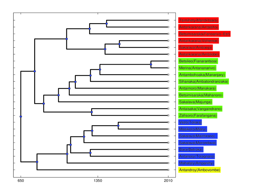
Figure 1: UPGMA tree for 23 Malagasy dialects, with hypothetical separation times. Variants are named by traditional dialect names followed by locations in parentheses. The four main branches are colored distinctively. The main separation of Malagasy dialects is center-north-east vs. south-west.

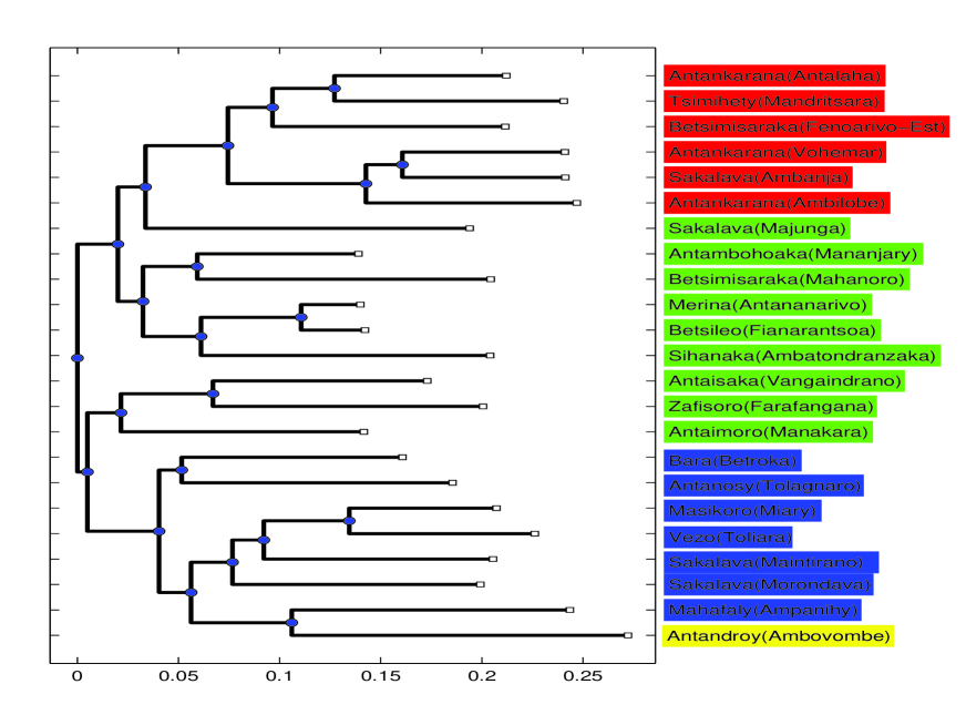
Figure 2: NJ tree for 23 Malagasy dialects. Colors compare with the UPGMA tree in Fig. 1. The graph confirms the main center-north-east vs. south-west division. The main difference is that three dialects at the linguistic border are grouped differently. Colors facilitate a rapid comparison.

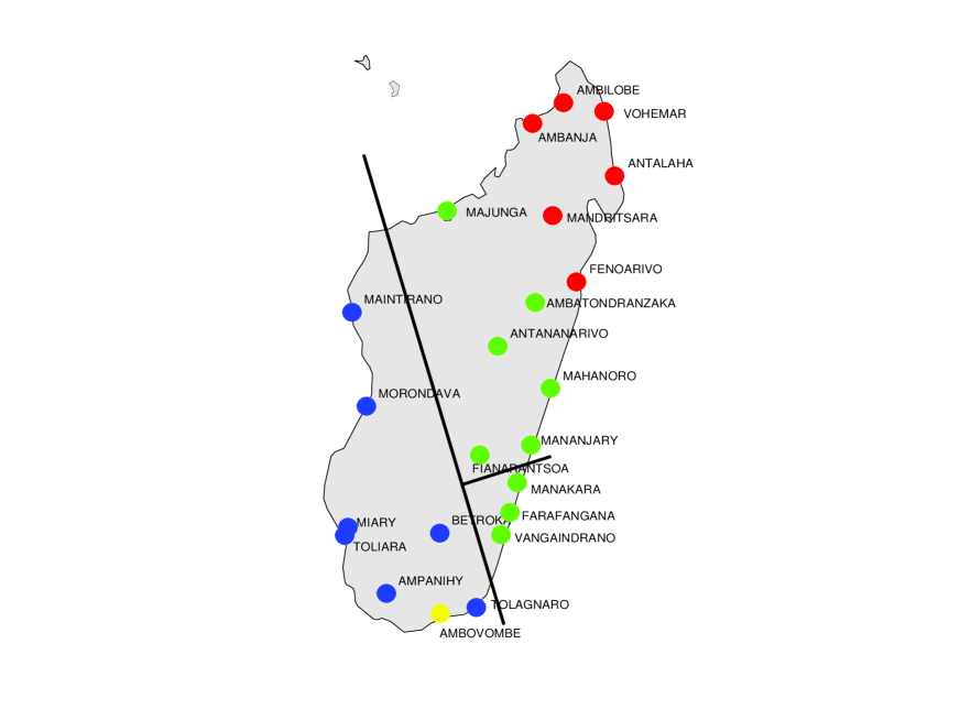
Figure 3: Geographical locations of the 23 dialects studied, with colors showing the main dialect branches according to Fig. 1. The straight line running from the south-east to the north-west of the island corresponds to the basic split in UPGMA tree while the NJ grouping is similar but Manakara, Farafangana and Vaingandrano are grouped with south-west.

The two algorithms used are the Neighbor-Joining (NJ) [Saitou and Nei, 1987] and the Unweighted Pair Group Method with Arithmetic Mean (UPGMA) [Sokal and Michener, 1958]. The main theoretical difference between the algorithms is that UPGMA assumes that evolutionary rates are the same on all branches of the tree, while NJ allows differences in evolutionary rates. The question of which method is better at inferring the phylogeny has been studied by running various simulations where the true phylogeny is known. Most of these studies were in biology but at least one [Barbançon et al, 2006] specifically tried to emulate linguistic data. Most of the studies (starting with [Saitou and Nei, 1987] and including [Barbançon et al, 2006]) found that NJ usually came closer to the true phylogeny. Since in our case, the relations among dialects are not necessarily tree-like, it is desirable to test the different methods against empirical linguistic data, which is mainly why trees derived by means of both methods are presented here.

The input data for the UPGMA tree are the pairwise separation times obtained from lexical distances by a rule [Serva and Petroni, 2008] which is a simple generalization of the fundamental formula of glottochronology. The absolute time-scale is calibrated by the results of the SCA analysis (see below), which indicate a separation date of A.D. 650. While the scale below the UPGMA tree (Fig. 1) refers to separation times, the scale below the NJ tree (Fig. 2) simply shows lexical distance from the root. The LDN distance between two language variants is roughly equal to the sum of their lexical distance from their closest common node.

Since UPGMA assumes equal evolutionary rates, the ends of all the branches line up on the right side of the UPGMA tree. The assumption of equal rates also determines the root of the tree on the left side. NJ allows unequal rates, so the ends of the branches do not all line up on the NJ tree. The extent to which they fail to line up indicates how variable the rates are. The tree is rooted by the midpoint (the point in the network equidistant from the two most distant dialects) but we also checked that the same result is obtained following the standard strategy of adding an out-group.

There is a good fit between geographical position of dialects (see Fig. 3) and their position both in the UPGMA (Fig. 1) and NJ trees (Fig. 2). In both trees the dialects are divided into two main groups (colored blue and yellow vs. red and green in Fig. 1).

Given the consensus between the two methods, the result regarding the basic split can be considered solid. Geographically the division corresponds to a border running from the south-east to the north-west of the island, as shown in Fig. 3 where the UPGMA and NJ main separation lines are drawn. A major difference concerns the Vangaindrano, Farafangana and Manakara dialects, which have shifting allegiances with respect to the two main groups under the different analyses. Additionally, there are minor differences in the way that the two main groups are configured internally. Most strikingly, we observe that in the UPGMA tree Majunga is grouped with the central dialects while in the NJ tree it is grouped with the northern ones. This indeterminacy would seem to relate to the fact that the town of Majunga is at the geographical border of the two regions.

Another difference is that in the UPGMA tree the Ambovombe variant of the dialect traditionally called Antandroy is quite isolated, whereas in the NJ tree Ambovombe and the Ampanihy variant of Mahafaly group together. Since the UPGMA algorithm is a strict bottom-up approach to the construction of a phylogeny, where the closest taxa are joined first, it will tend to treat the overall most deviant variant last. This explains the differential placement of Ambovombe in the two trees. The length of the branch leading to the node that joins Ambovombe and Ampanihy in the NJ tree shows that these two variants have quite a lot of similarities but in the UPGMA method these similarities in a sense ’drown’ in the differences that set Ambovombe off from other Malagasy variants as a whole.

As a further confirmation of this analysis we also computed the average LDN distance from each dialect to all the others. Antandroy has the largest average distance, confirming that it is the overall most deviant variant (something which is also commonly pointed out by other Malagasy speakers). We further note that the smallest average distance is for the official variant, that of Merina. This may probably be explained, at least in part, as an effect of the convergence of other variants towards this standard.

2.2 The results of Vérin et al. (1969)

Our classification results, including the grouping of the dialects in a south-west and a center-east-north cluster, differ from [Vérin et al, 1969]’s interpretation of their results, according to which there is a major split between the dialects on the northern tip of the island and all the rest.

This divergence is somewhat surprising, so let us look into the way that Vérin et al. proceeded. There are some differences in the way that theirs and our datasets were constructed and the coverage. Vérin et al. used a 100-item Swadesh list, while we use a larger set of 200 words. We include locations that Vérin et al. did not cover. Moreover, following [Gudschinsky, 1956], Vérin et al. (1969: 35) exclude Bantu loanwords from consideration, whereas we treat loanwords on a par with inherited words (in practice, however, Vérin et al.. only seem to identify one form as Bantu, namely amboa ’dog’. Finally, a major difference is that Vérin et al. evaluated distances by the standard glottochronological approach based on cognate counting whereas we use the LDN measure.

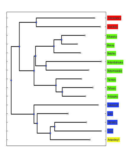
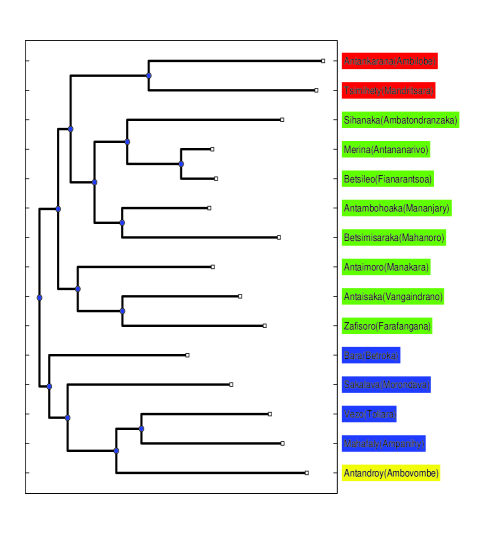
Figure 4: Comparison between NJ trees based on respectively data collected by [Vérin et al, 1969] (left) and by ourselves (right). The tree with Vérin data (Fig. 4a) is obtained by the standard lexicostatistical approach while the tree with our data (Fig. 4b) uses LDN distances. Names of variants for the left tree are those of [Vérin et al, 1969], but the correspondence with our naming scheme, which makes use of to dialect names and towns, is evident.

In spite of these differences our results are in reality quite similar to those of Vérin et al., the differences mainly relating to the interpretation of their results. The great leap from results to interpretation is due to the fact that Vérin et al. did not have the kinds of sophisticated phylogenetic methods at their disposal for deriving a classification from a matrix of cognacy scores that are available today. Their method for constructing trees goes something like this: cluster the closest dialects first, using some threshold. Then move the threshold and join dialects or dialect groups under deeper nodes. Different trees can be constructed from using different thresholds. One of the problems with this approach, not addressed by the authors, is that it assumes a constant rate of change. For instance in one of their trees (their Chart 1 on p. 59) Merina, Sihanaka, and Betsileo Ambositra are joined under one node attached at the 92% cognacy level. The actual percentages, however, do not fit a constant rate scenario (a.k.a. ’ultrametricality’): Sihanaka and Merina share 92% cognates, Betsileo Ambositra and Merina also share 92%, but Sihanaka and Betsileo Ambositra only share 86%. No solution to this problem is given (and, indeed, it is a problem for any phylogenetic algorithm that cannot be ’solved’ but at least needs to be addressed). Instead, violations of ultrametricality seem to be dealt with in an ad hoc way. In the case of the example just given Sihanaka and Betsileo Ambositra are treated as if they also shared 92% cognates. Since the principles used by Vérin et al.. to derive their trees are unclear there is no need to discuss their trees in detail. Moreover, each tree differs from the next, making it difficult to summarize the claims embodied in these trees. Some generalizations, however, do emerge. The Antankarana dialect in the far north constitutes its own isolated branch in all three trees, and in all three trees there are three sets of dialects that always belong together on different nodes: (1) Merina, Sihanaka, Betsileo Ambositra, Betsimisaraka; (2) Taimoro, Antaisaka, Zafisoro; (3) Mahafaly, Antandroy-1. Other dialects have no particularly close relationship to any other dialect, or else exhibit shifting allegiances.

In Fig. 4a we subject the distances data of Vérin et al. to NJ. Using this method each of the clusters (1-3) also turns up, but joined by other dialects which could not be safely placed at any deeper level of embedding by Vérin et al.. Thus, their clustering method essentially throws out so much information that only about half of the dialects become meaningfully classified. The most problematical aspect of their interpretation, however, is that there is supposed to be a fundamental split between the Antankarana dialect in the far north of the island and all other dialects. As we demonstrate in Fig. 4a, this is not borne out by the data, but is an artifact of the clustering method.

The NJ interpretation of the results of Vérin et al. (Fig. 4a) may be compared to our own results obtained from the LDN distances evaluated using our own data (Fig. 4b). Only variants belonging to the intersection of the two datasets are included. Names of variants are made identical, using the names from Vérin et al. The Betsimisaraka list from our data is the one from Mahanoro and the Antankarana list is the one from Vohemar.

The two trees have similar topologies, in particular, the main partition in both cases separates center-north-east from south-west dialects, which is at the variance the interpretation of Vérin et al. of their results. It is remarkable that the differences between the two trees are so minor considering differences both in the data and in the methods for calculating differences among dialects.

Fig. 4b was produced by using the same input LDN distances and the same NJ algorithm as used for Fig. 2. Comparing the two trees we observe that the simple reduction of the number of input dialects has the effect of modifying the position of Farafangana, Vankaindrano and Manakara variants (compare Fig. 4b with Fig. 2). Indeed, the NJ tree in Fig. 4b based on 15 dialects shows the same main branching as the UPGMA tree in Fig. 1, which differs from that of the NJ tree in Fig. 2 based on 23 dialects. This instability of tree topology caused by the number of input dialects and the differences in algorithms (UPGMA vs. NJ) shows that a tree structure is not optimal for capturing all the information contained in the set of lexical distances. Thus, we consider a different, geometrically-based approach, presented in the following section, necessary for a verification of classification results.

3 Geometric representation of Malagasy dialects

Although tree diagrams have become ubiquitous in representations of language taxonomies, they fail to reveal the full complexity of affinities among languages. The reason is that the simple relation of ancestry, which is the single principle behind a branching family tree model, cannot grasp the complex social, cultural and political factors molding the evolution of languages [Heggarty, 2006]. Since all dialects within a group interact with each other and with the languages of other families in ’real time’, it is obvious that any historical development in languages cannot be described only in terms of pair-wise interactions, but reflects a genuine higher order influence, which can best be assessed by Structural Component Analysis (SCA). This is a powerful tool which represents the relationships among different languages in a language family geometrically, in terms of distances and angles, as in the Euclidean geometry of everyday intuition. Being a version of the kernel PCA method [Schölkopf et al, 1998], it generalizes PCA to cases where we are interested in principal components obtained by taking all higher-order correlations between data instances. It has so far been tested through the construction of language taxonomies for fifty major languages of the Indo-European and Austronesian language families [Blanchard et al, 2010a]. The details of the SCA method are given in the Appendix B.

In Fig. 5 we show the three-dimensional geometric representation of 23 dialects of the Malagasy language and the Maanyan language, which is closely related to Malagasy. The three-dimensional space is spanned by the three major data traits ($\{q_{2},q_{3},q_{4}\}$, see Appendix B for details) detected in the matrix of linguistic LDN distances.

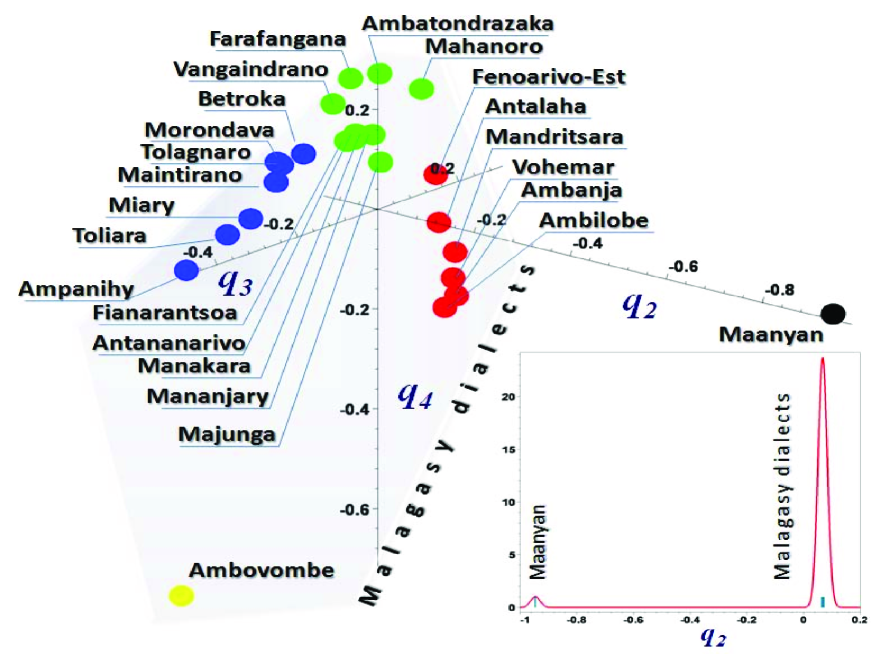
Figure 5: The three-dimensional geometric representation of the Malagasy dialects and the Maanyan language in the space of major data traits ($q_{2},q_{3},q_{4}$) shows a remarkable geographical patterning separating the northern (red) and the southern (blue) dialect groups, which fork from the central part of the island (the dialects spoken in the central part are colored green, while Antandroy is yellow). The kernel density estimate of the distribution of the $q_{2}$ coordinates, together with the absolute data frequencies, indicate that all Malagasy dialects belong to a single plane orthogonal to the data trait of the Maanyan language ($q_{2}$).

The clear geographical patterning is perhaps the most remarkable aspect of the geometric representation. The structural components reveal themselves in Fig. 5 as two well-separated spines representing both the northern (red) and the southern (blue) dialects of entire language. It is remarkable that all Malagasy dialects belong to a single plane orthogonal to the data trait of the Maanyan language ($q_{2}$). The plane of Malagasy dialects is attested by the sharp distribution of the language points in Cartesian coordinates along the data trait $q_{2}.$ This color point of Malagasy dialects over their common plane is shown in Fig. 6 where a reference azimuth angle $\varphi$ is introduced in order to underline the evident symmetry. It is important to mention that although the language point of Antandroy (Ambovombe) is located on the same plane as the rest of Malagasy dialects, it is situated far away from them and obviously belongs to neither of the dialect branches and for this reason is not reported in the next figure to be discussed (Fig. 6). This clear SCA isolation of Antrandroy is compatible with its position in the tree in Fig. 1.

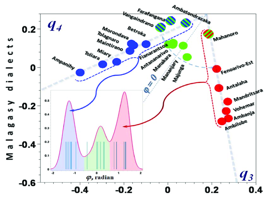
Figure 6: The plane of Malagasy dialects ($q_{3},q_{4}$); Antandroy (Ambovombe) is excluded. The kernel density estimate of the distribution over azimuth angles, together with the absolute data frequencies, allows the rest of Malagasy dialects to be classified into the three groups: north (red), south-west (blue), and center (green).

The distribution of language points supports the main conclusion following from the UPGMA and NJ methods (Figs. 1-2) of a division of the main group of Malagasy dialects into three groups: north (red), south-west (blue) and center (green). These clusters are evident from the representation shown in Fig. 6. However, with respect to the classification of some individual dialects the SCA method differs from the UPGMA and NJ results. Since their azimuthal coordinates better fit the general trend of the southern group, the Vangaindrano, Farafangana, and Ambatontrazaka dialects spoken in the central part of the island are now grouped with the southern dialects (blue) rather than the central ones (see Sec. 2). Similarly, the Mahanoro dialect is now classified in the northern group (red), since it is best fitted to the northern group azimuth angle. The remaining five dialects of the central group (green colored) are characterized by the azimuth angles close to a bisector ($\varphi=0$).

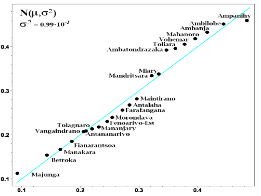
Figure 7: The radial coordinates are ranked and then plotted against their expected values under normality. Departures from linearity, which signify departures from normality, is minimal.

4 The Arrival to Madagascar

4.1 Dating the arrival

The radial coordinate of a dialect is simply the distance of its representative point from the origin of coordinates in Fig. 5. It can be verified that the position of Malagasy dialects along the radial direction is remarkably heterogeneous indicating that the rates of change in the Swadesh vocabulary was anything but constant.

The radial coordinates have been ranked and then plotted in Fig. 7 against their expected values under normality, such that departures from linearity signify departures from normality. The dialect points in Fig. 7 show very good agreement with univariate normality with the value of variance $\sigma^{2}=0.99\times 10^{-3}$ which results from the best fit of the data. This normal behaviour can be justified by the hypothesis that the dialect vocabularies are the result of a gradual and cumulative process in which many small, independent innovations have emerged and to which they have additively contributed.

In the SCA method, which is based on the statistical evaluation of differences among the items of the Swadesh list, a complex nexus of processes behind the emergence and differentiation of dialects is described by the single degree of freedom (as another degree of freedom, the azimuth angle, is fixed by the dialect group) along the radial direction [Blanchard et al, 2010b].

The univariate normal distribution (Fig. 7) implies a homogeneous diffusion time evolution in one dimension, under which variance $\sigma^{2}\propto t$ grows linearly with time. The locations of dialect points would not be distributed normally if in the long run the value of variance $\sigma^{2}$ did not grow with time at an approximately constant rate. We stress that the constant rate of increase in the variance of radial positions of languages in the geometrical representation (Fig. 5) has nothing to do with the traditional glottochronological assumption about the constant replacement rate of cognates assumed by the UPGMA method.

It is also important to mention that the value of variance $\sigma^{2}=0.99\times 10^{-3}$ calculated for the Malagasy dialects does not correspond to physical time but rather gives a statistically consistent estimate of age for the group of dialects. In order to assess the pace of variance changes with physical time and to calibrate the dating method we have used historically attested events. Although the lack of documented historical events makes the direct calibration of the method difficult, we suggest (following [Blanchard et al, 2010a]) that variance evaluated over the Swadesh vocabulary proceeds approximately at the same pace uniformly for all human societies. For calibrating the dating mechanism in [Blanchard et al, 2010a], we have used the following four anchoring historical events (see [Fouracre:2007]) for the Indo-European language family: i.) the last Celtic migration (to the Balkans and Asia Minor) (by 300 BC); ii.) the division of the Roman Empire (by 500 AD); iii.) the migration of German tribes to the Danube River (by 100 AD); iv.) the establishment of the Avars Khaganate (by 590 AD) causing the spread of Slavic people. It is remarkable that all of the events mentioned uniformly indicate a very slow variance pace of a millionth per year, $t/\sigma^{2}=(1.367\pm 0.002)\cdot 10^{6}.$ This time-age ratio returns $t=1,353$ years if applied to the Malagasy dialects, suggesting that landing in Madagascar was around 650 A.D. This is in complete agreement with the prevalent opinion among scholars including the influential one of Adelaar [Adelaar, 2009].

4.2 The landing area

In order to hypothetically infer the original center of dispersal of Malagasy variants, we here use a variant of the method of [Wichmann et al, 2010a]. This method draws upon a well-known idea from biology [Vavilov, 1926] and linguistics [Sapir, 1916] that the homeland of a biological species or a language group corresponds to the current area of greatest diversity. In [Wichmann et al, 2010a] this idea is transformed into quantifiable terms in the following way. For each language variant a diversity index is calculated as the average of the proportions between linguistic and geographical distances from the given language variant to each of the other language variants (cf. [Wichmann et al, 2010a] for more detail). The geographical distance is defined as the great-circle distance (i.e., as the crow flies) measured by angle radians. In this paper we adopt a variant of the method described in more detail in Appendix C.

The result of applying this method to Malagasy variants is that the best candidate for the homeland is the south-east coast where the three most diverse towns, i.e., Farafangana, Mahanoro and Ambovombe, are located, and where the surrounding towns are also highly diverse. The northern locations are the least diverse and they must have been settled last.

A convenient way of displaying the results on a map is shown in Fig. 8, where location are indicated by means of circles with different color gradations. The greater the diversity of a location is, the darker the color. The figure suggest that the landing would have occurred somewhere between Mahanoro (central part of the east cost) and Ambovobe (extreme south of the east coast), the most probable location being in the center of this area, where Farafangana is situated. Finally, we have checked that if the entire Greater Barito East group is considered, the homeland of Malagasy stays in the same place, but becomes secondary with respect to the south Borneo homeland of the group.

The identification of a linguistic homeland for Malagasy on the south-eastern coast of Madagascar receives some independent support from unexpected kinds of evidence. According to [Faublée, 1983] there is an Indian Ocean current that connects Sumatra with Madagascar. When Mount Krakatoa exploded in 1883, pumice was washed ashore on Madagascar’s east coast where the Mananjary River opens into the sea (between Farafangana and Mahanoro). During World War II the same area saw the arrival of pieces of wreckage from ships sailing between Java and Sumatra that had been bombed by the Japanese air-force. The mouth of the Mananjary River is where the town of Manajary is presently located, and it is in the highly diverse south-east coast as shown in Fig. 8. To enter the current that would eventually carry them to the east coast of Madagascar the ancestors of today’s Malagasy people would likely have passed by the easily navigable Sunda strait.

In his studies on the roots of Malagasy, Adelaar finds that the language has an important contingent of loanwords from Sulawesi (Buginese) [Adelaar, 1995b, Adelaar, 2009]. We have also compared Malagasy (and its dialects) with various Indonesian languages. While we unsurprisingly find that Maanyan is the closest language, we also find that Buginese is the third closest one (see also [Petroni and Serva, 2008]). The similarity with Buginese appears to be a further argument in favor of the southern path through the Sunda strait to Madagascar. In fact, if the Malay sailors recruited their crew in Borneo and, at a limited extent, in Sulawesi, they likely crossed this strait before starting their navigation in the open waters.

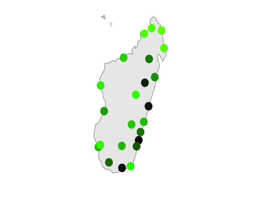
Figure 8: The homeland of Malagasy dialects as determined through diversity measures. The darkest-colored towns have the highest diversity values while the light-colored the lowest. The most diverse area is the south-east coast where landing would have occurred, the less diverse area in the north, indicating that this area was settled last.

Furthermore, we found that the dialects of Manajary, Manakara, Antananarivo and Fianarantsoa are noticeably closer both to Maanyan and Malay with respect to the other variants. Manajary and Manakara are both in the identified landing area in the south-east coast while Antananarivo and Fianarantsoa are in the central highlands of Madagascar. This fact may suggest that landing was followed shortly after by a migration to the interior of the Island.

5 Conclusion and outlook

All results in this paper rely on two main ingredients: a new dataset from 23 different variants of the language and an automated method to evaluate lexical distances. Analyzing the distances through different types of phylogenetic algorithm (NJ and UPGMA) as well as through a geometrical approach we find that all approaches converge on a result where dialects are classified into two main geographical subgroups: south-west vs. center-north-east. It is not clear, at this stage, if this main division is caused by geography or by an early splitting of the population into two different subpopulations or even by a colonization history with more than one founding nucleus. The last hypothesis, however, is somewhat unlikely given the relative uniformity of the dialects.

An output of the geometric representation of the distribution of the dialects is a landing date of around 650 AD, in agreement with a view commonly held by students of Malagasy. Furthermore, by means of a technique which is based on the calculation of differences in linguistic diversity, we propose that the south-east coast was the location were the first colonizers landed. This location also suggests that the path followed by the sailors went from Borneo, through the Sunda strait, and subsequently, along major oceanic currents, to Madagascar.

Finally, we measured the distance of the Malagasy variants to other Indonesian languages and found that the dialects of Manajary, Manakara, Antananarivo and Fianarantsoa are noticeably closer to most of them.

A larger comparison of Malagasy variants with Indonesian (and possibly African) languages is desirable. Although Malagasy is assigned to the the Greater East Barito group it has many loanwords from other Indonesian languages such as Javanese, Buginese, and Malay, especially in the domains of maritime life and navigation. It has also been observed that it is unlikely that Maanyan speaking Dayaks were responsible for the spectacular migrations from Kalimantan to Madagascar since they are forest dwellers with river navigation skills only. Furthermore, many manifestations of Malagasy culture cannot be linked up with the culture of the Dayaks of the south-east Barito area. For example, the Malagasy people use outrigger canoes, whereas south-east Barito Dayaks never do; some of the Malagasy musical instruments are very similar to musical instruments in Sulawesi; and some of the Malagasy cultigens (wet rice) cannot be found among Barito river inhabitants. In contrast, some funeral rites, such as the famadihana (second burial), are similar to those of Dayaks. Nevertheless, it should be observed that it is not clear whether the above cultural traits are specific to a region or a people or whether they are generic traits that can be found sporadically in other Austronesian cultures.

Non-Maanyan cultural and linguistic traits raise several questions concerning the ancestry of the Malagasy people. Assuming that Dayaks were brought as subordinates together with a few other Indonesians by Malay seafarers, they formed the majority in the initial group and their language constituted the core element of what later became Malagasy. In this way Malagasy would have absorbed words of the Austronesian languages of the other slaves and of the Malay seafarers. Is this a sufficient explanation, or are things are more complicated? For example, may we hypothesize two or more founding colonies with different ethnic composition? And is it possible that later specific contacts altered the characteristics of some local dialects?

In order to answer these questions it is necessary to make a careful comparison of all Malagasy variants with all Austronesian languages. A dialect may provide information about the pre-migratory composition of its speakers and also about further external contributions due to successive landing of Indonesian sailors.

Furthermore, the island was almost surely inhabited before the arrival of Malagasy ancestors. Malagasy mythology portrays a people, called the Vazimba, as the original inhabitants, and it is not clear whether they were part of a previous Austronesian expansion or a population of a completely different origin (Bantu, Khoisan?). Is it possible to track the aboriginal vocabulary into the some of the dialects such as, for example, Mikea (see [Blench, 2010])?

These questions call for a new look at the Malagasy language, not as a single entity, but as a constellation of variants whose histories are still to be fully understood.

Appendix A

The lexical distance [Serva and Petroni, 2008, Petroni and Serva, 2008, Holman et al, 2008] between the two languages, $l_{i}$ and $l_{j}$, is computed as the average of the normalized Levenshtein (edit) distance [Levenshtein, 1966] over the vocabulary of 200 items,

$$D\left(l_{i},l_{j}\right)\,\,=\,\,\frac{1}{200}\sum_{\alpha=1}^{200}\frac{\left\|w_{i}(\alpha),w_{j}(\alpha)\right\|}{\max\left(\left|w_{i}(\alpha)\right|,\left|w_{j}(\alpha)\right|\right)}.$$ (1)

where the item is indicated by $\alpha$, $\left\|w_{i}(\alpha),w_{j}(\alpha)\right\|$ is the standard Levenshtein distance between the words $w_{i}(\alpha)$ and $w_{j}(\alpha)$, and $|w_{i}(\alpha)|$ is the number of characters in the word $w_{i}(\alpha)$ . The sum runs over all the 200 different items of the Swadesh list. Assuming that the number of languages (or dialects) to be compared is $N$, then the distances $D(l_{i},l_{j})$ are the entries of a $N\times N$ symmetric matrix ${\bf D}$ (obviously $D(l_{i},l_{i})=0$).

The matrix, with entries multiplied by 1000, is the following:

1
2	323
3	246	276
4	322	240	295
5	302	281	309	345
6	227	318	275	359	266
7	413	386	390	418	314	370
8	280	386	342	401	356	245	436
9	366	424	379	412	405	375	450	409
10	411	396	416	440	318	366	249	456	482
11	207	326	260	362	286	061	383	201	374	384
12	362	343	345	387	292	328	289	397	435	330	324
13	303	369	330	381	384	329	454	362	256	487	318	407
14	343	302	331	355	243	317	303	403	423	314	336	301	419
15	397	453	394	462	392	375	342	463	485	304	383	405	471	388
16	368	391	385	416	392	390	448	406	320	474	383	429	325	418	486
17	400	350	369	390	280	358	165	433	427	278	373	240	439	261	358	410
18	322	376	325	374	391	337	426	381	198	473	339	412	234	406	461	264	414
19	358	407	376	417	408	394	440	419	292	481	387	431	325	422	472	161	408	243
20	297	388	359	430	356	299	400	346	386	433	275	375	363	375	455	348	394	349	355
21	386	341	370	385	290	344	262	403	422	321	348	250	404	306	403	401	213	416	417	383
22	225	389	332	394	382	316	471	319	385	475	287	421	296	431	480	382	467	348	387	356	441
23	379	424	407	424	398	380	443	433	315	466	380	412	351	420	472	203	395	288	202	351	409	406
	1	2	3	4	5	6	7	8	9	10	11	12	13	14	15	16	17	18	19	20	21	22

where the number-variant correspondence is:

1 Antambohoaka (Mananjary), 2 Antaisaka (Vangaindrano), 3 Antaimoro (Manakara), 4 Zafisoro (Farafangana), 5 Bara (Betroka), 6 Betsileo (Fianarantsoa), 7 Vezo (Toliara), 8 Sihanaka (Ambatondranzaka), 9 Tsimihety (Mandritsara), 10 Mahafaly (Ampanihy), 11 Merina (Antananarivo), 12 Sakalava (Morondava), 13 Betsimisaraka (Fenoarivo-Est), 14 Antanosy (Tolagnaro), 15 Antandroy (Ambovombe), 16 Antankarana (Vohemar), 17 Masikoro (Miary), 18 Antankarana (Antalaha), 19 Sakalava (Ambanja), 20 Sakalava (Majunga), 21 Sakalava (Maintirano), 22 Betsimisaraka (Mahanoro), 23 Antankarana (Ambilobe).

Appendix B

The lexical distance (1) between two languages, $l_{i}$ and $l_{j}$, can be interpreted as the average probability to distinguish them by a mismatch between two characters randomly chosen from the orthographic realizations of the vocabulary meanings. There are infinitely many matrices that match all the structure of ${\bf D}$, and therefore contain all the information about the relationships between languages, [Blanchard et al, 2010a]. It is remarkable that all these matrices are related to each other by means of a linear transformation,

$${\bf T}\,\,=\,\,{\bf\Delta}^{-1}{\bf D},\quad{\bf\Delta}=\mathrm{diag}\left(\sum_{k=1}^{N}D\left(l_{1},l_{k}\right)\ldots\sum_{k=1}^{N}D\left(l_{N},l_{k}\right)\right),$$ (2)

which can be interpreted as a random walk [Blanchard et al, 2010a, Blanchard et al, 2010b] defined on the weighted undirected graph determined by the matrix of lexical distances ${\bf D}$ over the $N$ different languages. Random walks defined by the transition matrix (2) describe the statistics of a sequential process of language classification. Namely, while the elements $T(l_{i},l_{j})$ of the matrix ${\bf T}$ evaluate the probability of successful differentiation of the language $l_{i}$ provided the language $l_{j}$ has been identified certainly, the elements of the squared matrix ${\bf T}^{2}$, ascertain the successful differentiation of the language $l_{i}$ from $l_{j}$ through an intermediate language, the elements of the matrix ${\bf T}^{3}$ give the probabilities to differentiate the language through two intermediate steps, and so on. The whole host of complex and indirect relationships between orthographic representations of the vocabulary meanings encoded in the matrix of lexical distances (1) is uncovered by the von Neuman series estimating the characteristic time of successful classification for any two languages in the database over a language family,

$${\bf J}\,\,=\,\,\lim_{n\to\infty}\sum_{k=0}^{n}{\bf T}^{n}\,\,=\,\,\frac{1}{1-{\bf T}}.$$ (3)

The last equality in (3) is understood as the group generalized inverse (Blanchard:2010b) being a symmetric, positive semi-definite matrix which plays the essentially same role for the SCA, as the covariance matrix does for the usual PCA analysis. The standard goal of a component analysis (minimization of the data redundancy quantified by the off-diagonal elements of the kernel matrix) is readily achieved by solving an eigenvalue problem for the matrix ${\bf J}$. Each column vector $q_{k}$, which determines a direction where $\bf J$ acts as a simple rescaling, ${\bf J}q_{k}=\lambda_{k}q_{k}$, with some real eigenvalue $\lambda_{k}=0$, is associated to the virtually independent trait in the matrix of lexical distances ${\bf D}$. Independent components $\left\{q_{k}\right\}$, $k=1,\ldots N$, define an orthonormal basis in $\mathbb{R}^{N}$ which specifies each language $l_{i}$ by $N$ numerical coordinates, $l_{i}\to\left(q_{1,i},q_{2,i},\ldots q_{N,i}\right)$. Languages that cast in the same mold in accordance with the $N$ individual data features are revealed by geometric proximity in Euclidean space spanned by the eigenvectors $\left\{q_{k}\right\}$ that might be either exploited visually, or accounted analytically. The rank-ordering of data traits $\left\{q_{k}\right\}$, in accordance to their eigenvalues, $\lambda_{0}=\lambda_{1}<\lambda_{2}=\ldots=\lambda_{N}$, provides us with the natural geometric framework for dimensionality reduction. At variance with the standard PCA analysis [Jolliffe, 2002], where the largest eigenvalues of the covariance matrix are used in order to identify the principal components, while building language taxonomy, we are interested in detecting the groups of the most similar languages, with respect to the selected group of features. The components of maximal similarity are identified with the eigenvectors belonging to the smallest non-trivial eigenvalues. Since the minimal eigenvalue $\lambda_{1}=0$ corresponds to the vector of stationary distribution of random walks and thus contains no information about components, we have used the three consecutive components $\left(q_{2,i},q_{3,i},q_{4,i}\right)$ as the three Cartesian coordinates of a language $l_{i}$ in order to build a three-dimensional geometric representation of language taxonomy. Points symbolizing different languages in space of the three major data traits are contiguous if the orthographic representations of the vocabulary meanings in these languages are similar.

Appendix C

The lexical distance $D(l_{i},l_{j})$ between two dialects $l_{i}$ and $l_{j}$ was previously defined; their geographical distance $\Delta(l_{i},l_{j})$ can be simply defined as the distance between the two locations where the dialects were collected. There are different possible measure units for $\Delta(l_{i},l_{j})$. We simply use the great-circle angle (the angle that the two location form with the center of the earth).

It is reasonable to assume, in general, that larger geographical distances correspond to larger lexical distances and vice-versa For this reason in [Wichmann et al, 2010a] the diversity was measured as the average of the ratios between lexical and geographical distance. This definition implicitly assumes that lexical distances vanish when geographical distances equal 0. Nevertheless, different dialects are often spoken at the same locations, separated by negligible geographical distances. For this reason, and because a zero denominator in the division involving geographical distances would cause some diversity indexes to become infinite, [Wichmann et al, 2010a] arbitrarily added a constant of .01 km to all distances.

Here we similarly add a constant, but one whose value is better motivated. We plotted all the $\frac{23\times 22}{2}=253$ points $\Delta(l_{i},l_{j}),\,D(l_{i},l_{j})$ in a bi-dimensional space and verified that the pattern is compatible with a linear shape in the domain of small geographical distances. Linear regression of the $20\%$ of points with smaller geographical distances gives the interpolating straight line $D=a+b\Delta$ with $a=0.22$ and $b=0.04$. The results indicates that a lexical distance of $0.22$ is expected between two variants of a language spoken in coinciding locations.

The choice of constants $a$ and $b$ by linear regression assures that the ratio between $D(l_{i},l_{j})$ and $a+b\Delta(l_{i},l_{j})$ is around 1 for any pair of dialects $l_{i}$ and $l_{j}$. A large value of the ratio corresponds to a pair of variants which are lexically more distant and vice-versa. It is straightforward to define the diversity of a dialect as

$$V(l_{i})\,\,=\,\,\frac{1}{22}\sum_{j\neq i}\frac{D(l_{i},l_{j})}{a+b\Delta(l_{i},l_{j})}.$$ (4)

in this way, locations with high diversity will be characterized by a a larger $V(l_{i})$, while locations with low diversity will have a smaller one.

Notice that the above definition coincides with the one in [Wichmann et al, 2010a], the main difference being that instead of an arbitrary value of $a$ we obtain it through the output of linear regression.

The diversities (in a decreasing order), computed with (4), are the following: Zafisoro (Farafangana): 1.00, Betsimisaraka (Mahanoro): 0.98, Antandroy (Ambovombe): 0.98, Sihanaka (Ambatontrazaka): 0.95, Antaisaka (Vangaindrano): 0.92, Mahafaly (Ampanihy): 0.90, Tsimihety (Mandritsara): 0.90, Antaimoro (Manakara): 0.90, Betsimisaraka (Fenoarivo-Est): 0.88, Sakalava (Morondava): 0.87, Antambohoaka (Mananjary): 0.86, Vezo (Toliara): 0.86, Bara (Betroka): 0.86, Sakalava (Majunga): 0.85, Betsileo (Fianarantsoa): 0.85, Antanosy (Tolagnaro): 0.83, Sakalava (Maintirano): 0.83, Masikoro (Miary): 0.82, Merina (Antananarivo): 0.82, Sakalava (Ambanja): 0.77, Antankarana (Ambilobe): 0.77, Antankarana (Antalaha): 0.76, Antankarana (Vohemar): 0.74.

Appendix D

In Table 1 below we provide information on the people who furnished the data collected by one of us (M.S.) at the beginning of 2010 with the invaluable help of Joselinà Soafara Néré. For any dialect (except for Merina, for which published lists combined with the personal knowledge of M.S. were used), data were elicited independently from two consultants. Their names and birth dates follow each of the dialect names.

Table 1: People who furnished the data on Malagasy dialects

MERINA
(ANTANANARIVO)	SERVA Maurizio
ANTANOSY	SOAFARA Joselina Nere	08 November 1987
(TOLAGNARO)	ETONO Imasinoro Lucia	18 February 1982
BETSIMISARAKA	ANDREA Chanchette Généviane	07 August 1985
(FENOARIVO-EST)	RAZAKAMAHEFA Joachim Julien	09 November 1977
SAKALAVA	SEBASTIEN Doret	26 November 1980
(MORONDAVA)	RATSIMANAVAKY Christelle J.	29 February 1984
VEZO	RAKOTONDRABE Justin	02 August 1972
(TOLIARA)	RASOAVAVATIANA Claudia S.	28 June 1983
ZAFISIRO	RALAMBO Alison	11 June 1982
(FARAFANGANA)	RAZANAMALALA Jeanine	03 February 1980
ANTAIMORO	RAZAFENDRALAMBO Haingotiana	24 July 1985
(MANAKARA)	RANDRIAMITSANGANA Blaise	05 February 1989
ANTAISAKA	RAMAHATOKITSARA Fidel Justin	24 April 1984
(VANGAINDRANO)	FARATIANA Marie Luise	17 August 1990
ANTAMBOHOAKA	RAKOTOMANANA Roger	04 May 1979
(MANANJARY)	ZAFISOA Raly	20 April 1983
BETSILEO	RAMAMONJISOA Andrininina Leon Fidelis	16 April 1987
(FIANARANTSOA)	RAKOTOZAFY Teza	25 December 1985
BARA	RANDRIANTENAINA Hery Oskar Jean	17 Jenuary 1986
(BETROKA)	NATHANOEL Fife Luther	26 May 1983
TSIMIHETY	RAEZAKA Francis	23 December 1984
(MANDRITSARA)	FRANCINE Germaine Sylvia	04 May 1985
MAHAFALY	VELONJARA Larissa	21 April 1989
(AMPANIHY)	NOMENDRAZAKA Christian	07 June 1982
SIHANAKA	ARINAIVO Robert Andry	06 Jenuary 1979
(AMBATONDRAZAKA)	RONDRONIAINA Natacha	27 December 1985
ANTANKARANA	ANDRIANANTENAINA N. Benoit	06 August 1984
(VOHEMAR)	EDVINA Paulette	28 Jenuary 1982
ANTANKARANA	RANDRIANARIVELO Jean Ives	24 December 1986
(ANTALAHA)	RAZANAMIHARY Saia	07 September 1985
SAKALAVA	CASIMIR Jaozara Pacific	03 April 1983
(AMBANJA)	ZAKAVOLA M. Sandra	17 July 1984
SAKALAVA	RATSIMBAZAFY Serge	17 May 1978
(MAJUNGA)	VAVINIRINA Fideline	23 June 1970
ANTANDROY	RASAMIMANANA Z. Epaminodas	05 June 1983
(AMBOVOMBE)	MALALATAHINA Tiaray Samiarivola	07 July 1984
MASIKORO	MAHATSANGA Fitahia	22 March 1976
(ANTALAHA)	VOANGHY Sidonie Antoinnette	12 October 1981
ANTANKARANA	BAOHITA Maianne	21 August 1984
(AMBILOBE)	NOMENJANA HARY Jean Pierre Felix	07 June 1980
SAKALAVA	HANTASOA Marie Edvige	02 November 1985
(MAINTIRANO)	KOTOVAO Bernard	06 October 1983
BETSIMISARAKA	RASOLONANDRASANA Voahirana	24 September 1985
(MAHANORO)	ANDRIANANDRASANA Maurice	03 April 1979

References

- [Adelaar, 1995a] A. Adelaar, Asian roots of the Malagasy; A linguistic perspective. In: Bijdragen tot de Taal-, Land- en Volkenkunde 151, no: 3, Leiden, 325-356 (1995).
- [Adelaar, 1995b] A. Adelaar, Borneo as a Cross-Roads for Comparative Austronesian Linguistics. In The Austronesians in history. J. F. Bellwood, and D. Tryon editors, 75-95 (1995). Australian National University, ANU E Press.
- [Adelaar, 2009] A. Adelaar, Loanwords in Malagasy. In Loanwords in the World’s Languages: A Comparative Handbook, M. Haspelmath and U. Tadmor editors, 717-746 (2009). Berlin: De Gruyter Mouton.
- [Bakker et al, 2009] D. Bakker, A. Müller, V. Vellupillai, S. Wichmann, C. H. Brown, P. Brown, D. Egerov, R. Mailhammer, A. Grant and E. W. Holman, Adding typology to lexicostatistics: a combined approach to language classification. Linguistic Typology 13, 167-179 (2009).
- [Barbançon et al, 2006] F. Barbançon, T. Warnow, S. N. Evans, D. Ringe, and L. Nakhleh, An experimental study comparing linguistic phylogenetic reconstruction methods. Paper presented at the conference Languages and Genes, UC Santa Barbara, September 8-10, (2006), http://www.cs.rice.edu/ nakhleh/Papers/UCSB09.pdf.
- [Blanchard et al, 2010a] Ph. Blanchard, F. Petroni, M. Serva and D. Volchenkov, Geometric Representations of Language Taxonomies. Computer Speech & Language doi:10.1016/j.csl.2010.05.003 (published on-line 21 May 2010).
- [Blanchard et al, 2010b] Ph. Blanchard, J.-R. Dawin, D. Volchenkov, Markov Chains or the Game of Structure and Chance: From Complex Networks, to Language Evolution, to Musical Compositions. European Physical Journal - Special Topics 184, 1-82 (2010).
- [Blench, 2010] R. M. Blench, The vocabularies of Vazimba and Beosi: do they represent the languages of the pre-Austronesian populations of Madagascar? Preprint, Cambridge (2010)
- [Blench and Walsh, 2009] R. M. Blench and M. Walsh, Faunal names in Malagasy: their etymologies and implications for the prehistory of the East African Coast. In Eleventh International Conference on Austronesian Linguistics (11 ICAL), Aussois, France, (2009).
- [Dahl, 1951] O. C. Dahl, Malgache et Maanjan: une comparaison linguistique. Olso: Egede Instituttet (1951).
- [Dahl, 1991] O. C. Dahl, Migration from Kalimantan to Madagascar. Oslo: The Institute of Comparative Research in Human Culture, Norwegian University Press.
- [Dyen, 1953] I. Dyen, Review of Otto Dahl, Malgache et Maanjan. Language 29.4, 577-590 (1953).
- [Faublée, 1983] J. Faublée, Mémoire spécial du Centre d’études sur le monde arabe et du Centre d’études sur l’océan occidental, 21-30 (1983). Paris: INALCO & Conseil International de la language française.
- [Fouracre:2007] P. Fouracre, The New Cambridge Medieval History, Cambridge University Press (1995-2007).
- [Greenhill et al, 2009] S. J. Greenhill, R. Blust, and R.D. Gray, The Austronesian Basic Vocabulary Database. http://language.psy.auckland.ac.nz/austronesian, (2003-2009).
- [Gudschinsky, 1956] S. Gudschinsky, The ABC’s of lexicostatistics (glottochronology). Word 12, 175-210 (1956).
- [Heggarty, 2006] P. Heggarty, Interdisciplinary indiscipline? Can phylogenetic methods meaningfully be applied to language data and to dating language? In Phylogenetic Methods and the Prehistory of Languages, P. Forster and C. Renfrew editors, p. 183, McDonald Institute for Archaeological Research, Cambridge (2006).
- [Holman et al, 2008] E. W. Holman, S. Wichmann, C. H. Brown, V. Velupillai, A. Müller, and D. Bakker, Explorations in automated language comparison. Folia Linguistica 42.2, 331-354 (2008).
- [Houtman, 1603] F. Houtman, Spraeckende woord-boeck inde Maleysche ende Madagascarsche talen met vele Arabische ende Turcsche woorden. Amsterdam: Jan Evertsz (1603).
- [Hurles et al 2005] M. E. Hurles, B. C. Sykes, M. A. Jobling and P. Forster, The dual origin of the Malagasy in Island Southeast Asia and East Africa: Evidence from maternal and paternal lineages. American Journal of Human Genetics 76, 894-901 (2005).
- [Jolliffe, 2002] I. T. Jolliffe, Principal Component Analysis. Springer Series in Statistics XXIX, 2nd ed. (2002), Springer, NY.
- [Levenshtein, 1966] V. I. Levenshtein, Binary codes capable of correcting deletions, insertions and reversals. Soviet Physics Doklady 10, 707 (1966).
- [Mariano, 1613-14] L. Mariano, Rélation du voyage de decouverte fait à l’île Saint-Laurent dans les années 1613-1614. In Collection des ouvrages anciens concernant Madagascar, ed. by A. and G. Grandidier, 2: 1-64 (1613-1614). Paris, Comité de Madagascar.
- [Petroni and Serva, 2008] F. Petroni and M. Serva, Languages distance and tree reconstruction. Journal of Statistical Mechanics: theory and experiment, P08012 (2008).
- [Petroni and Serva, 2010] F. Petroni and M. Serva, Measures of lexical distance between languages. Physica A 389, 2280-2283 (2010).
- [Saitou and Nei, 1987] N. Saitou and M. Nei, The neighbor-joining method: a new method for reconstructing phylogenetic trees. Molecular Biology and Evolution 40, 406-425 (1987).
- [Sapir, 1916] E. Sapir, Time Perspective in Aboriginal American Culture, a Study in Method. Geological Survey Memoir 90: No. 13 (1916). Anthropological Series. Ottawa: Government Printing Bureau.
- [Schölkopf et al, 1998] B. Schölkopf, A.J. Smola and K.-R. Müller, Nonlinear component analysis as a kernel eigenvalue problem. Neural Computation 10, 1299 (1998).
- [Serva and Petroni, 2008] M. Serva and F. Petroni, Indo-European languages tree by Levenshtein distance. EuroPhysics Letters 81, 68005 (2008).
- [Serva and Petroni, 2011] M. Serva and F. Petroni, Dialects of Malagasy. (2011). http://univaq.it/ serva/languages/languages.html.
- [Sokal and Michener, 1958] R. Sokal and C. D. Michener, A statistical method for evaluating systematic relationships. University of Kansas Science Bulletin 38, 1409-1438 (1958).
- [Tuuk, 1864] H. N. van der Tuuk, Outlines of grammar of Malagasy language. Journal of the Royal Asiatic Society 8.2 (1864).
- [Vavilov, 1926] N. I. Vavilov, Centers of origin of cultivated plants. Trudi po Prikl. Bot. Genet. Selek. [Bulletin of Applied Botany and Genetics] 16, 139-248 (1926).
- [Vérin et al, 1969] P. Vérin, C.P. Kottak and P. Gorlin, The glottochronology of Malagasy speech communities. Oceanic Linguistics 8, 26-83 (1969).
- [Wichmann et al, 2010a] S. Wichmann, A. Müller and V. Velupillai, Homelands of the world’s language families. Diachronica 27.2, 247-276 (2010).
- [Wichmann et al 2010b] S. Wichmann, E. W. Holman, D. Bakker and C.H. Brown, Evaluating linguistic distance measures. Physica A 389, 3632-3639 (2010).
- [Wichmann et al, 2010c] S. Wichmann, A. Müller, V. Velupillai, C. H. Brown, E. W. Holman, P. Brown, S. Sauppe, O. Belyaev, M. Urban, Z. Molochieva, A. Wett, D. Bakker, J-M List, D. Egorov, R. Mailhammer, D.Beck and H. Geyer, The ASJP Database (version 13), (2010), http://email.eva.mpg.de/ wichmann/languages.htm.