A threshold induced phase transition in the kinetic exchange models
Abstract
We study an ideal-gas-like model where the particles exchange energy stochastically, through energy conserving scattering processes, which take place if and only if at least one of the two particles has energy below a certain energy threshold (interactions are initiated by such low energy particles). This model has an intriguing phase transition in the sense that there is a critical value of the energy threshold, below which the number of particles in the steady state goes to zero, and above which the average number of particles in the steady state is non-zero. This phase transition is associated with standard features like “critical slowing down” and non-trivial values of some critical exponents characterizing the variation of thermodynamic quantities near the threshold energy. The features are exhibited not only in the mean field version but also in the lattice versions.
pacs:
05.20.-y, 87.23.Ge, 05.70.FhI Introduction
The kinetic theory of gases had played a pivotal role in the development of statistical mechanics, which is more than a century old. This theory describes a gas as a collection of a large number of particles (atoms or molecules) which are constantly in random motion, and these rapidly moving particles constantly collide with each other and exchange energy. In the ideal gas, this energy is only kinetic. Recently physicists have been studying two-body kinetic exchange models in the socio-economic contexts in the rapidly growing interdisciplinary field of “Sociophysics” CCCbook2006 and “Econophysics” SCCCbook2010 . The two-body exchange dynamics has been developed in the context of modeling income, money or wealth distributions in a society Yakovenko2009 ; Arnab2007 ; Patriarca2010 ; Chakraborti2010a ; Redner2010 ; Chatterjee2004a ; Chakraborti2000a ; Chakraborti2009 , and modeling opinion formation in the society Mehdi2010 ; LCCC2010 ; CC2010 ; Sen , analogous to the kinetic theory model of ideal gases. These studies have given deeper insights and different perspectives in the simple physics of two body kinetic exchange dynamics. In this context of wealth exchange processes, Iglesias et al. Iglesias-physica ; Iglesias-sc&cul had considered a model for the economy where the poorest in the society (atom with least energy in the gas) at any stage takes the initiative to go for a trade (random wealth / energy exchange) with anyone else. Interestingly, in the steady state, one obtained a self-organized poverty line, below which none could be found and above which, a standard exponential decay of the distribution (Gibbs) was obtained.
Here, we study a model where particles, interact among themselves through two-body energy () conserving stochastic scatterings with at least one of the particles having energy below a threshold (poverty line in the equivalent economic model). The states of particles are characterized by the energy , such that and the total energy is conserved (= here, such that the average energy of the system ). The evolution of the system is carried out according to the following dynamics:
| (1) |
where (threshold energy or “ poverty line”) and is a stochastic variable, changing with time (scattering). It can be noticed that, the quantity is conserved during each collision: . The question of interest is: “What is the steady state distribution of energy in such systems?”
In the standard case, when the threshold energy goes to infinity (), we know that the steady state energy distribution will be the exponential Gibbs distribution () Yakovenko2009 . However, when a finite threshold energy is introduced (), several new and intriguing features appear. These features are exhibited not only in the mean field version (with infinite-range interaction, pairs of particles randomly chosen from particles) but also in the lattice versions (with nearest neighbor interactions, i.e. exchanges between the nearest neighbors on lattice sites).
II Model simulations and results
II.1 The Model
We simulate a system of particles (agents). At any time , we select randomly a particle . If the energy of the particle is below a prescribed threshold energy , then it collides with any other random particle (in the mean field model) which can have any energy whatsoever, and the two particles will exchange energy according to the Gibbs-Boltzmann dynamics of Eq. (1). After each such successful collision, the time is incremented by unity. The dynamics will continue for an indefinite period, unless there is no particle left below the threshold energy, in which case the dynamics will freeze. If the dynamics gets frozen (when for all ), we employ a ‘mild’ perturbation such that a randomly chosen particle will be dropped to the lower level () by giving up its energy to anyone else (to ensure total energy conservation). It can be shown that the addition of this perturbation does not alter the relevant quantities for a thermodynamically large systems, and simply ensures ergodicity in the system. After sufficiently large time , a steady state is reached when the energy distribution (and also other average quantities) do not change with time. We start with different initial random configurations, where the states of particles are characterized by the energies , which are drawn randomly from an uniform distribution such that and the average energy is set to unity. We find the system to be ergodic (the steady state distribution is independent of the initial conditions ), and we take steady state averages over all such independent initial conditions to evaluate the quantities of interest.
We study mainly three cases (a) mean field (or infinite range) case where and in Eq. (1) can represent any two particles/agents in the system; (b) one dimensional case where along a chain and (c) two dimensional case, where where represents neighbors of . In our studies we consider a 2D-square lattice.
We observe that for finite values of the energy threshold , the steady state energy distribution is no longer the simple Gibbs-Boltzmann distribution. We also find that (), the average number of particles below the threshold energy in the steady state, is zero for values below or at a critical threshold energy , and for , is non-zero. The steady state value of , the average number of particles below the threshold energy is seen to act like an “order parameter” of the system. We study the relaxation dynamics in the system: the relaxation of to the steady state value of ( for , the “relaxation time”). We find grows as approaches , and eventually diverges at . The details of the results are given below.
II.2 Results: Mean field model
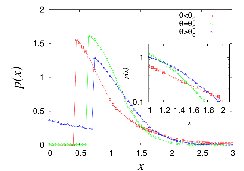
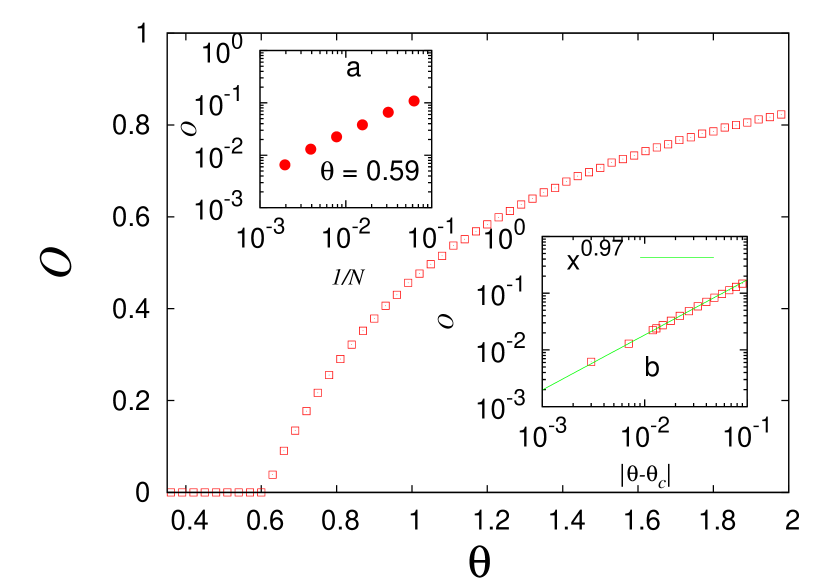
In the mean field (long range) model, we first look for any particle () with energy and then this particle is allowed to interact with any other particle (), following Eq. (1). This continues until either the steady state, or a frozen state with for all is reached. In the case of frozen state, as mentioned earlier, any one particle is picked up randomly and it loses its energy to any other (randomly chosen) particle, and goes below the threshold . This induces further dynamics. Eventually steady state is reached. We study this steady state energy distribution (see Fig. 1 ), and the order parameter (see Fig. 2), showing a “phase transition” at . A power law fit gives .
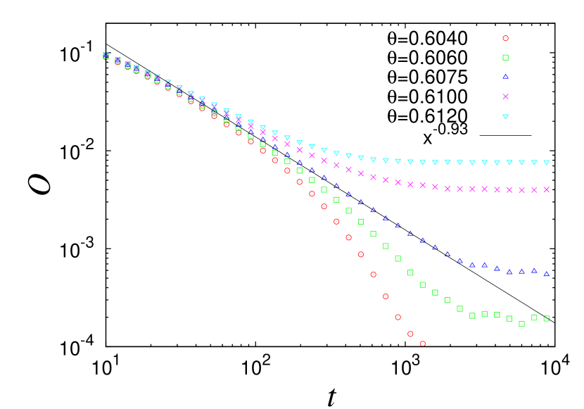
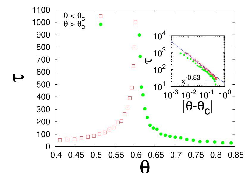
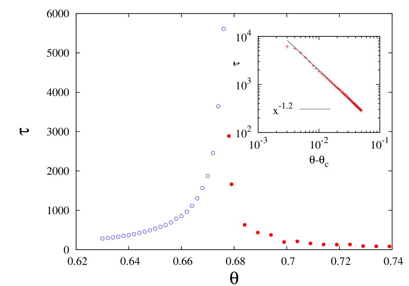
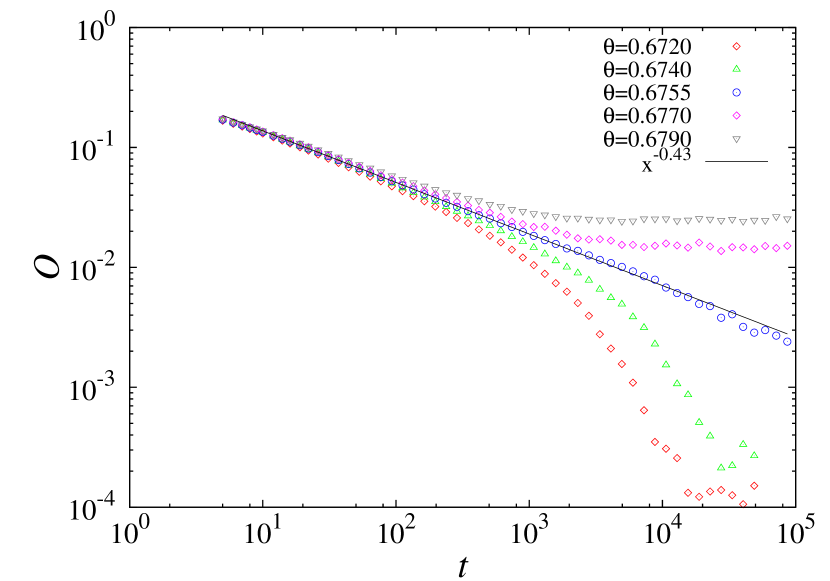
We also studied the relaxation behavior of . At , the variation fits well with ; (see Fig. 3). The relaxation time is estimated numerically from the time value at which first touches the steady state value within a pre-assigned error limit. We find diverging growth of relaxation time near (see Fig. 4), showing ‘critical slowing down’ at the critical value . The values of exponent for the divergence in have been estimated (for both and ). For the mean-field model, the fitting value for exponent .
We have also studied the universality of this behavior by generalizing the dynamics in Eq. (1) to
| (2) |
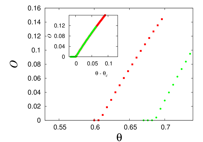
where and are the random stochastic variables within the range . The critical point shifts to ( for = = ). The transition behaviour is seen to be universal near the critical point , but the critical point depends specifically on the model (see Fig. 5).
II.3 Results: One dimensional model
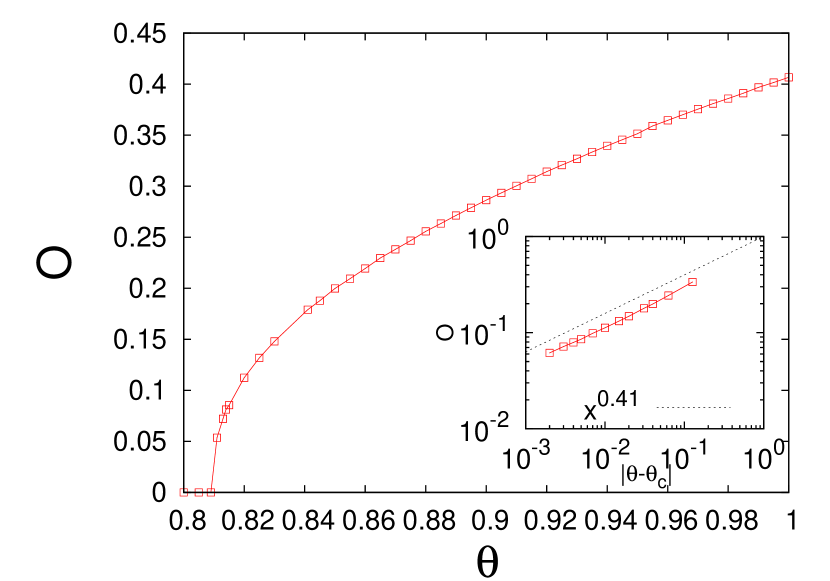
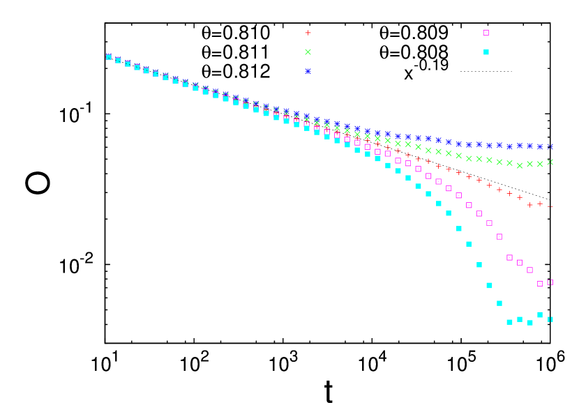
In one dimensional lattice version, the particles are arranged on a periodic chain. At any time , we randomly select a lattice site . If the energy of the corresponding particle is below a prescribed threshold energy , then it collides with any one randomly chosen nearest neighbors which can have any energy whatsoever, and the two particles will exchange energy according to Eq. (1). After each such successful collision, the time is incremented by unity. This process is continued until steady state is reached. The steady state order parameter variations against theshold is shown in Fig. 6, with exponent and . The fitting value for exponent turn out to be around (see Fig. 7). Also we find (see Fig. 8). It may be noted that a recent study of a related chain model with such energy cut-off for kinetics, where the effective temperature is varied, has been studied pk:2011 . Though the behavior is similar, the effective critical behavior (exponent values) seem to be quite different.

II.4 Results: Two dimensional model
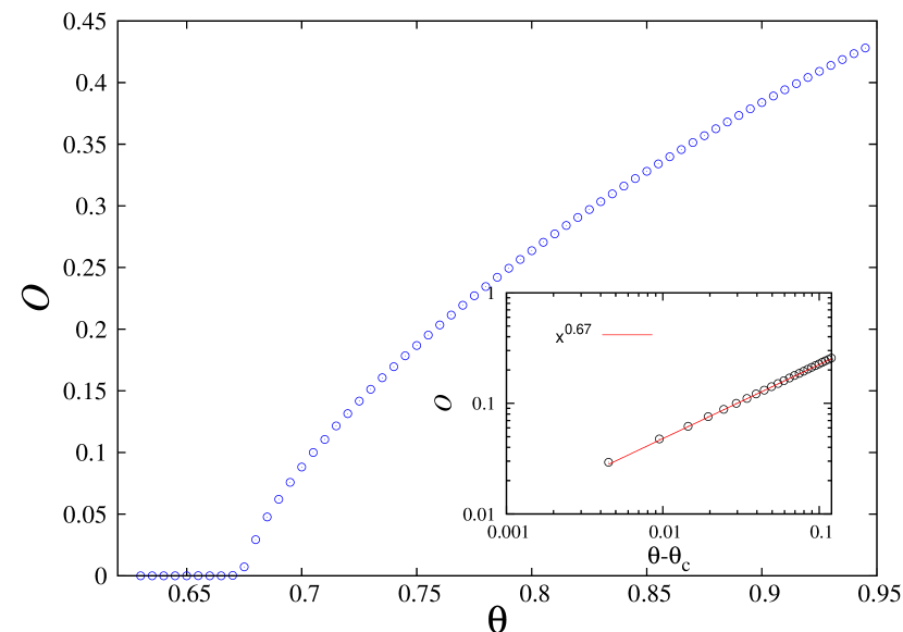
For the 2D lattice version, the particles are arranged on a square lattice, and this time one of the four nearest neighbors of is chosen randomly as particle . If the energy of the particle is below a prescribed threshold energy , then it collides with any one randomly chosen nearest neighbor which can have any energy whatsoever, and the two particles will exchange energy according to Eq. (1). After each such successful collision, the time is incremented by unity. This process is continued until steady state is reached. Variation of the steady state order parameter against theshold is shown in Fig. 9, with exponent and . Also, we find (see Fig. 10) and (see Fig. 11).
| This Model | Manna Model | ||
|---|---|---|---|
| 1D | 0.41 0.02 | 0.382 0.019 | |
| 2D | 0.67 0.01 | 0.639 0.009 | |
| MF | 0.97 0.01 | 1 | |
| 1D | 1.9 0.05 | 1.876 0.135 | |
| 2D | 1.2 0.01 | 1.22 0.029 | |
| MF | 0.83 0.01 | 1 | |
| 1D | 0.19 0.01 | 0.141 0.024 | |
| 2D | 0.43 0.02 | 0.419 0.015 | |
| MF | 0.93 0.01 | 1 |
All these estimated values of the critical exponents , , and are summarized in Table 1.
III Finite Size Effect
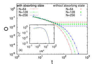
We have also studied the time variation of at different sizes () at . Plots of as a function of for different values of the system size (at critical point) are expected to collapse on a single curve. However, as we have used a special dynamics which never allows the system to fall in the absorbing state, in this case the activity saturates at a small steady value (see Fig. 12) instead of showing the finite size cut-off.
To study finite size effects in the decay of activity at the critical point, one has to remove the perturbation and allow the system to be trapped in the absorbing states. Using this dynamics, we have studied the effects of finite system size. Fig. 12, show the decay of with at the critical point for MF, , and systems, respectively. The insets in the corresponding figures show the data collapse. The fitting values of the exponent are and for MF, , and respectively, with values given in Table-I.


IV Summary & Discussion
Inspired by the success of the kinetic exchange models of market dynamics (see e.g., SCCCbook2010 ; Yakovenko2009 ; Arnab2007 ) and the observation that the poor or economically backwards in the society take major initiative in the market dynamics (see e.g., Iglesias-physica ; Iglesias-sc&cul and also Manna2010 ; Bak ), we consider an ideal-gas-like model of gas (or market) where at least one of the particles (or agents) has energy (money) less than a threshold (poverty line) value takes the initiative to scatter (trade) with any other particle (agent) in the system, following energy (money) conserving random processes (following Eq. (1)). For , the model reduces to the kinetic model of ideal gas with Gibbs distribution. The steady state is found to be ergodic (steady state results are independent of initial conditions). The perturbation employed in the frozen cases ( for all ) also does not affect significantly the thermodynamic quantities (e.g., the steady state value of for goes to 0 with , as can be seen from inset (a) of Fig. 2).
In general, we find that the steady state distribution (see Fig. 1 for the mean field, where each particle can interact irrespective of their distance from the active particle or agent having energy or money less than threshold or poverty line ) differs in form significantly from the Gibb’s distribution, for finite values of . The order parameter , giving the average fraction of particles (or agents) having energy (or money) below shows a phase transition behavior: for and for (see Fig. 2 for mean field, Fig. 6 for 1D, and Fig. 9 for 2D, respectively). The critical values are given by for mean field, 1D and 2D cases, respectively. The variation of near is quite universal (see Fig. 5). We find with for mean field, 1D and 2D cases, respectively. We also find that the relaxation time diverges strongly near as with for mean field, 1D and 2D cases, respectively. Finally, at , where for mean field, 1D and 2D cases, respectively (see Table 1).
It might be mentioned here that the above exponent values are indeed very close to those of the Manna Universality (MU) class (Lubeck:2004 ; see also Manna ; Menon ) in mean field, 1D, 2D cases: Our estimates for , and for mean field, 1D and 2D cases, respectively, are quite close to , and for corresponding MU cases; , and for mean field, 1D and 2D cases, are also close to , and in the corresponding MU cases. However, it may be noted that significant differences in the above estimates do exist. Also, for mean field, 1D and 2D cases might be compared with in the corresponding MU cases. These discrepancies could be due to finite size effect, and in that case the critical behavior of our model would belong to the MU class. As one can see, the estimated values of the exponents , and fit reasonably with the scaling relation within our limits of accuracy. In this connection, it is worth mentioning that the violation of the above scaling relation has also been observed Rossi , though such discrepancies seem to get removed if one uses all sample averages instead of averages over surviving samples Lee . In our case, however, this scaling relation seems to hold, as our simulation results correspond to all sample averages.
In summary, when the energy threshold is introduced in the kinetic theory of ideal gas such that the stochastic energy conserving scatterings between any two particles can take place only when one has energy less than , the gas system shows an intriguing dynamic phase transition at , having the exponent values in the mean field (long range scattering exchange), one dimension and two dimension, as estimated here using Monte Carlo simulation, are given in Table I.
Acknowledgements.
We are grateful to Arnab Chatterjee and Gautam Menon for useful comments on the critical behaviour of the model. We also acknowledge discussions with Mahashweta Basu, Rakesh Chatterjee and Soumyajyoti Biswas.References
- (1) (Eds.) B.K. Chakrabarti, A. Chakraborti and A. Chatterjee, Econophysics and Sociophysics: Trends and Perspectives (Wiley-VCH, Berlin, 2006).
- (2) S. Sinha, A. Chatterjee, A. Chakraborti and B.K. Chakrabarti, Econophysics: An Introduction (Wiley-VCH, Berlin, 2010).
- (3) V. Yakovenko, J. Rosser, Rev. Mod. Phys. 81, 1703 (2009).
- (4) A. Chatterjee, B.K. Chakrabarti, Eur. Phys. J. B 60, 135 (2007).
- (5) M. Patriarca, E. Heinsalu, A. Chakraborti, Eur. Phys. J. B 73, 145 (2010).
- (6) A. Chakraborti, I. Muni Toke, M. Patriarca, F. Abergel, Quantitative Finance, in press; available at arXiv:0909.1974v2 (2010).
- (7) P. L. Krapivsky, S. Redner, Science and Culture (Kolkata) 76, 424 (2010); arXiv:1006.4595 [physics.soc-ph].
- (8) A. Chakraborti, B.K. Chakrabarti, Eur. Phys. J. B 17, 167 (2000).
- (9) A. Chatterjee, B.K. Chakrabarti, S. S. Manna, Physica A 335, 155 (2004).
- (10) A. Chakraborti, M. Patriarca, Phys. Rev. Lett. 103, 228701 (2009).
- (11) M. Lallouache, A. Chakraborti and B.K. Chakrabarti, Science and Culture (Kolkata) 76, 485 (2010); arXiv:1006.5921 [physics.soc-ph].
- (12) M. Lallouache, A.S. Chakrabarti, A. Chakraborti and B.K. Chakrabarti, Phys. Rev. E 82, 056112 (2010).
- (13) A. Chakraborti and B.K. Chakrabarti, in Eds. F. Abergel, B.K. Chakrabarti, A. Chakraborti and M. Mitra, Econophysics of order-driven markets (Springer- Verlag (Italia), Milan, 2011).
- (14) P. Sen, Phys. Rev. E 83, 016108 (2011).
- (15) S. Pianegonda, J. R. Iglesias, G. Abramson and J. L. Vega, Physica A 322, 667 (2003).
- (16) J.R. Iglesias, Science and Culture (Kolkata) 76 , 437 (2010).
- (17) M. Basu, U. Gayen and P. K. Mohanty, arXiv.1102.1631v1.
- (18) S. Lübeck, Int. J. Mod. Phys. B 18, 3977 (2004).
- (19) A. Chakraborty, S. S. Manna Phys. Rev. E 81, 016111 (2010).
- (20) P. Bak and K. Sneppen, Phys. Rev. Lett. 71, 4083 (1993).
- (21) S. S. Manna, Physica A 179, 249(1991); S. S. Manna, J. Phys. A 24, L363 (1991).
- (22) G. I. Menon, S. Ramaswamy, Phys. Rev. E 79, 061108 (2009).
- (23) M. Rossi, R. Pastor-Satorras, and A. Vespignani Phys. Rev. Lett. 85, 1803 (2000).
- (24) S. B. Lee and S. G. Lee Phys. Rev. E 78, 040103(R) (2008).