We compute QCD corrections to the production of a $t\bar{t}$ pair in association with a hard photon at the Tevatron and the LHC. This process allows a direct measurement of the top quark electromagnetic couplings that, at the moment, are only loosely constrained. We include top quark decays, treating them in the narrow width approximation, and retain spin correlations of final-state particles. Photon radiation off top quark decay products is included in our calculation and yields a significant contribution to the cross-section. We study next-to-leading order QCD corrections to the $p\bar{p}\to t\bar{t}\gamma$ process at the Tevatron for the selection criteria used in a recent measurement by the CDF collaboration. We also discuss the impact of QCD corrections to the $pp\to t\bar{t}\gamma$ process on the measurement of the top quark electric charge at the $14$ TeV LHC.

QCD corrections to top quark pair production in association with a photon at hadron colliders

I Introduction

More than fifteen years after the discovery of the top quark, many of its quantum numbers are still not well-measured experimentally. For example, until recently qtmes it was possible to have a consistent description of “top” quark physics, assuming that the electric charge of the “top” quark is $Q_{t}=-4/3$, in contrast to its usual value $Q_{t}=2/3$ ma1 . By analyzing tracks of charged hadrons to estimate jet charges, the D0 collaboration excludes, at less than $2\sigma$ confidence level, the hypothesis that the event sample comes entirely from a heavy quark with the electric charge $Q_{t}=-4/3$. As pointed out in Ref. ub , a more direct way to measure the top quark charge is to study the production of a top quark pair in association with a hard photon. Indeed, to an extent that photons are only radiated off the top quarks, the rate for $t\bar{t}\gamma$ production is proportional to the square of the top quark electric charge. This assumption works well at the LHC, once photon radiation off top quark decay products is suppressed, but it fails at the Tevatron because top quark pair production there is dominated by $q\bar{q}$ annihilation.

The CDF collaboration has recently measured the cross-section of the process $p\bar{p}\to t\bar{t}\gamma$, searching for an excess in events that contain a lepton, a photon, $b$-jets and large missing energy cdf . Using $1.9~{}{\rm fb}^{-1}$ of data, they observed nine events that they interpreted as due to the $p\bar{p}\to t\bar{t}\gamma$ process. The analysis will be improved by using a larger data sample privatecom , so about fifty $t\bar{t}\gamma$ events can be expected in the near future. It is therefore important to have a reliable prediction for this process, including the possibility of applying selection criteria for final state particles used in Ref. cdf .

The authors of Refs. ub ; ub1 analyzed the potential of the Tevatron and the LHC to study electroweak couplings of the top quark, focusing on the $t\bar{t}Z$ and $t\bar{t}\gamma$ final states. If we neglect parity non-conservation, the interaction of top quarks with on-shell photons is described by two quantities – the electric charge $Q_{t}$ and the anomalous magnetic moment $a_{t}$. Both of these quantities can be studied in the $t\bar{t}\gamma$ production process. As shown in Refs. ub ; ub1 , the best sensitivity to $Q_{t}$ at the LHC is obtained if kinematic cuts force the photon to be emitted either in the production stage or in the decay stage. Because the non-vanishing anomalous magnetic moment of the top quark corresponds to a dimension-five non-renormalizable operator, it leads to a harder spectrum of photons in $pp(p\bar{p})\to t\bar{t}\gamma$. Given enough statistics, it should be possible to study this effect experimentally. Regardless of the details pertinent to a particular measurement, once selection criteria are specified, the study of top quark electromagnetic couplings becomes a counting experiment which may be subject to significant higher order QCD corrections. Therefore, the computation of next-to-leading order (NLO) QCD corrections to $t\bar{t}\gamma$ hadroproduction, that correctly incorporates decays of top quarks, becomes important.

NLO QCD corrections to the production of a $t\bar{t}$ pair and a hard photon in hadron collisions were recently calculated by Duan et al. ma . This computation was performed in the approximation of stable top quarks. While such an approximation gives an idea about the significance of higher order QCD effects for the production of $t\bar{t}\gamma$, it can not be used to find the magnitude of NLO QCD corrections when specific cuts are imposed on top quark decay products. As we explained in the previous paragraph, the ability to do this is important for a realistic analysis. In this paper, we extend the results of Ref. ma by computing NLO QCD corrections to $pp(p\bar{p})\to t\bar{t}+\gamma$, allowing for decays of top quarks. We note that radiative decays of top quarks are included into our analysis. To calculate one-loop virtual amplitudes, we employ the method of generalized $D$-dimensional unitarity suggested in Ref. Giele:2008ve and extended to massive particles in Ref. egkm . The current paper builds upon the previous studies of $t\bar{t}$ and $t\bar{t}+j$ production in hadron collisions, performed by two of us ms ; msj . Many technical aspects of the calculation are explained in those references and we do not repeat them here.

When top quarks are treated as truly unstable particles, non-factorizable QCD corrections appear my . Non-factorizable corrections imply a cross-talk between production and decays of top quarks; they can not be described in the narrow width approximation. It is well-understood by now my that, in many cases, these non-factorizable corrections lead to effects that are suppressed by ${\cal O}(\alpha_{s}\Gamma_{t}/m_{t})$, instead of the naive ${\cal O}(\alpha_{s})$ expectation for the suppression. Recently, the smallness of non-factorizable corrections in reactions with top quarks was confirmed by an explicit computation of the NLO QCD corrections to $pp(p\bar{p})\to W^{+}W^{-}b\bar{b}$ process that included both factorizable and non-factorizable contributions Denner:2010jp ; Bevilacqua:2010qb . In what follows we ignore the non-factorizable corrections and work in the on-shell approximation for top quarks.

As a final comment, we note that NLO QCD corrections are known for two other processes where the top quark pair is produced in association with color-neutral objects – $pp\to t\bar{t}H$ Beenakker:2002nc ; Dawson:2003zu and $pp\to t\bar{t}Z$ Lazopoulos:2008de — and to the production of a $t\bar{t}$ pair in association with one Dittmaier:2007wz ; Dittmaier:2008uj ; Bevilacqua:2010ve ; msj and two Bevilacqua:2010ve jets, as well as in association with a $b\bar{b}$ pair Bredenstein:2008zb ; Bredenstein:2009aj ; Bevilacqua:2009zn ; Bredenstein:2010rs . In all the cases, the NLO QCD corrections are calculated either assuming that all final state particles are stable, or treating QCD radiation in top decays incompletely. Similarly to the $t\bar{t}\gamma$ case, removing these omissions may become important for precision phenomenology, especially when aggressive cuts are involved to separate signals from backgrounds.

The remainder of the paper is organized as follows. In Section II we describe the setup of the calculation and present some results for the case when top quarks are treated as stable particles. In Section III we discuss the computation of NLO QCD corrections to radiative decays of top quarks. In Section IV we present phenomenological studies relevant for the Tevatron and the LHC, including decays of top quarks. We conclude in Section V. Technical details of the calculation are described in the Appendices.

II Production of a $t\bar{t}$ pair and a photon: stable top quarks

We first discuss the case of stable top quarks. To compute the NLO QCD corrections to $pp(p\bar{p})\to t\bar{t}\gamma$, we need to calculate one-loop virtual corrections and to account for the emission of an additional massless parton. For the calculation of the virtual corrections, we employ the method of generalized $D$-dimensional unitarity suggested in Ref. Giele:2008ve . This method has been used earlier by two of us in the computation of hadroproduction of $t\bar{t}+{\rm jet}$ in Ref. msj . To describe the $t\bar{t}\gamma$ final state, we can re-use much of that computation. For example, linear combinations of color-ordered one-loop amplitudes for $0\to t\bar{t}+3g$ msj give color-ordered amplitudes for $0\to t\bar{t}+2g+\gamma$ bdk . Similarly, color-ordered amplitudes for $0\to t\bar{t}+q\bar{q}+g$ msj can be used to construct color-ordered amplitudes for $0\to t\bar{t}+q\bar{q}+\gamma$. All the details of how amplitudes with gluons and quarks are transformed into amplitudes with gluons, quarks and a photon are given in Appendix A. We have checked our results for virtual corrections by re-calculating them, for a few phase-space points by using an independent implementation of the Ossola-Pittau-Papadopoulos (OPP) procedure opp , that we apply to individual Feynman diagrams. The Feynman diagrams are generated with the package FeynArts Hahn:2000kx .

The second, logically distinct part of any one-loop computation is the calculation of real emission corrections. When integrated over available phase-space, these corrections diverge. Such divergences must be removed by an appropriate procedure. We use the dipole formalism of Ref. Catani:1996vz extended to deal with QCD radiation off massive particles in Ref. Catani:2002hc . Dipoles relevant for our calculation can be found in Refs. Bevilacqua:2009zn ; mcfm ; Campbell:2005bb . In the actual implementation of the subtraction procedure, we closely follow Ref. mcfm . We have checked that our results do not depend on the parameter that restricts the integration over the dipole phase-space; this is a useful way to control the consistency of the implementation of the subtraction terms and to improve the efficiency of the computation nagy .

As we mentioned earlier, the calculation of NLO QCD corrections to $t\bar{t}\gamma$ production in hadronic collisions for stable top quarks was reported in Ref. ma . When we choose the setup of the calculation as close to Ref. ma as possible, we get good agreement with their results. However, some choices made in Ref. ma – for example the use of the electromagnetic coupling at the scale $M_{Z}$, the use of charm and bottom masses in the computation of the partonic channels $qg\to t\bar{t}\gamma+g$, $q=c,b$ and the three degree cut on the opening angle between the photon and the light quark in the final state – do not look very appealing to us. For this reason, we decided to present a number of results for cross-sections and kinematic distributions which can not be directly compared with the results reported in Ref. ma but which, we believe, correspond to more realistic choices of input parameters and better resemble details of experimental analyses.

Figure 1: Kinematic distributions in the production of a $t\bar{t}$ pair and a hard photon at the Tevatron, for stable top quarks. The bands correspond to the variation of the renormalization and factorization scales in the interval $m_{t}/2<\mu<2m_{t}$. Upper (lower) panes show $\bar{t}\;$ ($\gamma$) transverse momentum and rapidity distributions, respectively.

We now turn to the discussion of our results for the hadroproduction of a $t\bar{t}$ pair and a hard photon, for stable top quarks. Throughout the paper, we choose the top quark mass $m_{t}=172~{}{\rm GeV}$ and parton distribution functions CTEQ6L1 and CTEQ6.6M Pumplin:2002vw ; Nadolsky:2008zw for leading and next-to-leading computations, respectively. The strong coupling constant $\alpha_{s}$ is evaluated using one- and two-loop running with five massless flavors. To describe emission of the real photon, we use the fine structure constant $\alpha_{\rm QED}=1/137$. Although this choice should be self-evident because of QED Ward identities, we emphasize this fact because in many previous studies of the $t\bar{t}\gamma$ production, the cross-section was computed with $\alpha_{t\bar{t}\gamma}=\alpha_{\rm QED}(M_{Z})=1/128$. Using the correct value of the fine structure constant is numerically important because it decreases the prediction for the $t\bar{t}\gamma$ cross-section by about six percent.

For both the Tevatron and the LHC, we require that the photon is relatively hard $p_{\perp,\gamma}>20~{}{\rm GeV}$ and that it is isolated. To ensure that the implementation of photon isolation does not violate infra-red and collinear safety, we employ the procedure described in Ref. Frixione:1998jh . The photon is not considered isolated and events are rejected unless the condition

$$\sum\limits_{i\in{\rm partons}}E_{\perp,i}\;\theta\left(R-R_{i\gamma}\right)\leq E_{\perp,\gamma}\left(\frac{1-\cos(R)}{1-\cos(R_{\gamma j})}\right)$$ (1)

is fulfilled for cones of sizes $R$ that are smaller than $R_{\gamma j}=0.4$. In Eq.(1) $R_{\gamma i}$ is the photon-parton angular distance $R_{\gamma i}=\sqrt{(y_{\gamma}-y_{i})^{2}+(\varphi_{\gamma}-\varphi_{i})^{2}}$, where $y_{\gamma,i}$ ($\varphi_{\gamma,i})$ are the laboratory frame rapidities (azimuthal angles) of the photon and the parton $i$, respectively. Also, $E_{\perp,i}$ is the transverse energy of the parton $i$ and $E_{\perp,\gamma}$ is the transverse energy of the photon. We apply all other selection criteria to jets if and only if their separation from a photon exceeds $R_{\gamma j}$. A jet reconstructed inside the cone of size $R_{\gamma j}$ is not subject to selection criteria, see Ref. Frixione:1998jh . As our default, we set the renormalization and factorization scales equal to each other and choose them to be equal to the mass of the top quark $\mu=m_{t}$. We find the cross-section for $p\bar{p}\to t\bar{t}\gamma$ at the Tevatron ($\sqrt{s}=1.96~{}{\rm TeV}$) to be

$$\sigma_{\rm LO}=39.97^{+16.77}_{-10.91}~{}{\rm fb},\;\;\;\sigma_{\rm NLO}=37.6^{+0.8}_{-3.7}~{}{\rm fb},$$ (2)

where the lower value correspond to the scale set to $\mu=2m_{t}$ and the upper value to the scale set to $\mu=m_{t}/2$. QCD corrections greatly reduce the uncertainty in the predictions for the cross-section, changing it from about thirty percent at leading order to about ten percent at next-to-leading order. The cross-section for $pp\to t\bar{t}\gamma$ at the $14~{}{\rm TeV}$ LHC is

$$\sigma_{\rm LO}=1.96^{+0.64}_{-0.45}~{}{\rm pb},\;\;\;\sigma_{\rm NLO}=2.93^{+0.42}_{-0.39}~{}{\rm pb}.$$ (3)

The residual scale uncertainty in the NLO QCD cross-section at the LHC is about fifteen percent.

We note that results for $t\bar{t}\gamma$ production in Eqs.(2,3) show significant differences in the QCD corrections at the Tevatron and the LHC. At the scale $\mu=m_{t}$, the NLO QCD corrections decrease the $t\bar{t}\gamma$ cross-section by about six percent at the Tevatron and increase the $t\bar{t}\gamma$ cross-section by about $55\%$ at the LHC. It is peculiar that the magnitude of the NLO QCD corrections to $t\bar{t}\gamma$ production at the Tevatron and the LHC is very similar to the magnitude of the NLO QCD corrections to $t\bar{t}$ pair production. While the degree of the correlation between these corrections is perhaps somewhat surprising, it can be understood, at least partially, by considering emissions of soft photons which must factorize from the production process even when the NLO QCD corrections are included. This may also explain why a very similar pattern of QCD corrections was reported in Ref. ma , despite the fact that somewhat different input parameters are used in that computation.

Figure 2: Kinematic distributions in the production of a $t\bar{t}$ pair and a hard photon at the LHC, for stable top quarks. The bands correspond to the variation of the renormalization and factorization scales in the interval $m_{t}/2<\mu<2m_{t}$. Upper (lower) panes show $\bar{t}\;$ ($\gamma$) transverse momentum and rapidity distributions, respectively.

Kinematic distributions of top quark and photon transverse momenta and rapidities at the Tevatron and the LHC, are shown in Figs. 1,2. No dramatic changes in shapes of these distributions are observed. However, the rapidity distribution of top quarks at the Tevatron exhibits some interesting features. Indeed, in the process $p\bar{p}\to t\bar{t}\gamma$, photons can be emitted from both initial and final states. Interference of these emissions gives rise to a charge or forward-backward asymmetry of top quarks. We define

$$A_{t}=\frac{\sigma(y_{t}>0)-\sigma(y_{t}<0)}{\sigma(y_{t}>0)+\sigma(y_{t}<0)},$$ (4)

where $\displaystyle y_{t}=\frac{1}{2}\ln\left(\frac{E_{t}+p_{t,z}}{E_{t}-p_{t,z}}\right)$ is the rapidity of the top quark in the laboratory frame. As was pointed out in Ref. ma , the forward-backward asymmetry is significant. Calculating it in leading and next-to-leading order in perturbative QCD, with the parameters specified at the beginning of this Section, we obtain

$$A_{t,\rm LO}=-17.2^{+0.0}_{-0.0}\,\%,\;\;\;\;\;A_{t,\rm NLO}=-11.9^{+2.9}_{-1.3}\,\%,$$ (5)

where the central value corresponds to the renormalization and factorization scales set to $\mu=m_{t}$ and the lower(upper) value to $\mu=m_{t}/2$ and $\mu=2m_{t}$, respectively.

It is peculiar that the change in the NLO QCD asymmetry is nearly identical to the size of the NLO QCD corrections to forward-backward asymmetry in $p\bar{p}\to t\bar{t}j$, computed in Refs. Dittmaier:2007wz ; Dittmaier:2008uj ; msj . In fact, this similarity of NLO QCD corrections to the asymmetries in $p\bar{p}\to t\bar{t}\gamma$ and $p\bar{p}\to t\bar{t}j$ is easy to understand, following the observation of Ref. msj that large NLO QCD correction to the asymmetry in $p\bar{p}\to t\bar{t}j$ is related to the $5\%$ asymmetry in the inclusive rate for $p\bar{p}\to t\bar{t}$, first computed in Ref. kuhn .

III QCD corrections to radiative decays of top quarks

In this Section, we describe the computation of the NLO QCD corrections to the radiative decay of the top quark $t\to bW\gamma$. Since this is a relatively low-multiplicity process, the calculation of virtual corrections is performed using conventional Feynman diagrams, generated with FeynArts Hahn:2000kx , and the Passarino-Veltman reduction pv . For a few kinematic points, the results are checked against a computation based upon an independent implementation of the OPP procedure opp , that is applied to individual Feynman diagrams.

The real emission corrections to the decay rate are computed using the subtraction formalism described in Ref. ekt , in the context of non-radiative top decay $t\to bW$. However, the subtraction is also applicable to the radiative decay $t\to bW\gamma$ if one replaces the invariant mass of the $W$-boson with the invariant mass of the $W$-boson and the photon in all the relevant formulas in Ref. ekt . Specifically, the subtraction term, required to make the real emission contribution $t\to Wb\gamma+g$ integrable is given by the product of the matrix element squared for the process $t\to Wb\gamma$ and the dipole that reads ekt

$$D(p_{t},p_{g},p_{b})=4\pi\alpha_{s}\mu^{2\epsilon}C_{F}\left[\frac{1}{p_{b}p_{g}}\left(\frac{2}{1-z}-1-z-y\epsilon(1-z)\right)-\frac{m_{t}^{2}}{(p_{t}p_{g})^{2}}\right].$$ (6)

The kinematic variables used in Eq.(6) are defined through

$$p_{b}p_{g}=\frac{m_{t}^{2}}{2}(1-r)^{2}y,\;\;\;\;\;p_{t}p_{g}=\frac{m_{t}^{2}}{2}(1-r^{2})(1-z),$$ (7)

where $r^{2}=(p_{W}+p_{\gamma})^{2}/m_{t}^{2}$. In Ref. ekt , the dipole in Eq.(6) is integrated over the unresolved phase-space

$$\int\left[{\rm d}g\right]\;D(p_{t},p_{g},p_{b})={\cal N}\int\limits_{0}^{1}{\rm d}z\left(r^{2}+z(1-r^{2})\right)^{-\epsilon}\int\limits_{0}^{y_{\rm max}}{\rm d}yy^{-\epsilon}(y_{\rm max}-y)^{-\epsilon}D(p_{t},p_{g},p_{b}),$$ (8)

where $\epsilon=(4-d)/2$ is the parameter of the dimensional regularization, $d$ is the number of space-time dimensions and

$$y_{\rm max}=\frac{(1+r)^{2}z(1-z)}{z+r^{2}(1-z)},\;\;\;\;\;\;\;{\cal N}=\frac{(1-r)^{2}}{16\pi^{2}}m_{t}^{2-2\epsilon}\frac{(4\pi)^{\epsilon}}{\Gamma(1-\epsilon)}\left(\frac{1+r}{1-r}\right)^{2\epsilon}.$$ (9)

It is convenient to restrict the subtraction counter-terms to parts of the phase-space that are not too far from the singular limits nagy . If this is done, the subtraction terms need to be modified. Introducing such a modification in Eq.(6) and integrating over restricted phase-space, we find

$$\int\left[{\rm d}g\right]\;D(p_{t},p_{g},p_{b})\left[1-\theta(1-\alpha-z)\theta(y-\alpha y_{\rm max})\right]=$$

$$\frac{\alpha_{s}C_{F}}{2\pi}\frac{(4\pi\mu^{2})^{\epsilon}}{m_{t}^{2\epsilon}\Gamma(1-\epsilon)}\left[\frac{1}{\epsilon^{2}}+\frac{1}{\epsilon}\left(\frac{5}{2}-2\ln(1-r^{2})\right)+\frac{25}{4}+\frac{1}{2}\left(\frac{1}{(1-r^{2})^{2}}-\frac{8}{(1-r^{2})}+7\right)\ln r^{2}\right.$$

$$\left.+\frac{1}{2(1-r^{2})}+2{\rm Li}_{2}(1-r^{2})-\frac{5\pi^{2}}{6}-5\ln(1-r^{2})+2\ln^{2}(1-r^{2})+\frac{\eta}{2}\right.$$

$$\left.-2\ln^{2}\alpha-\left(\frac{7}{2}-4\alpha+\frac{\alpha^{2}}{2}\right)\ln\alpha+\frac{2(1-\alpha)r^{2}}{1-r^{2}}\ln\left(\frac{r^{2}}{1-\alpha+r^{2}\alpha}\right)\right].$$ (10)

We now present some numerical results for the QCD corrections to the radiative decay of the top quark $t\to bW\gamma$. We use $\alpha_{s}(m_{t})=0.107691$, which corresponds to the CTEQ NLO value of the strong coupling constant at $\mu=M_{Z}$ supplemented with the two-loop running to $\mu=m_{t}$. We take the mass of the $W$-boson to be $M_{W}=80.419~{}{\rm GeV}$. We work in the top quark rest frame and require the photon energy $E_{\gamma}$ to be larger than $10~{}{\rm GeV}$ and the opening angle between the momentum of the bottom quark and the photon to be such that $\cos\theta_{b\gamma}<0.98$. With these input parameters, we obtain the radiative decay width of the top quark $t\to bW\gamma$ at leading and next-to-leading order in perturbative QCD

$$\Gamma_{\rm LO}=4.48~{}{\rm MeV},\;\;\;\;\Gamma_{\rm NLO}=3.89~{}{\rm MeV}.$$ (11)

For the choice of the kinematic cuts described above, the QCD radiative corrections decrease radiative decay width by thirteen percent. This is similar to, but somewhat larger than, the magnitude of the NLO QCD corrections to the top quark decay width $t\to bW$, which decrease the decay width $t\to Wb$ by about eight percent.

In Fig. 3, we show distributions of the opening angle between the bottom quark and the photon and of the photon energy, and ratios of NLO and LO distributions. Shapes of these distributions are perfectly described by leading order computations; the NLO QCD corrections provide an overall renormalization factor. The distribution of the photon energy shows canonical enhancement of the soft photon emission probability at low $E_{\gamma}$, while the distribution in the opening angle shows a collinear enhancement peak at small relative angles between the bottom quark and the photon. Suppressing emissions from bottom quarks is important for the analysis of the top quark charge that we discuss in the next Section; a simple way to accomplish this is to require that the $b$-jet and the hard photon are sufficiently separated.

Figure 3: Kinematic distributions in radiative decays of top quarks $t\to Wb\gamma$. Upper panes show normalized distributions of the cosine of the angle between the $b$-quark and the photon and of the photon energy, computed through NLO QCD. Lower panes show ratios of NLO and LO kinematic distributions.

IV Production of a $t\bar{t}$ pair and a photon: unstable top quarks

A realistic description of the hadroproduction of the $t\bar{t}\gamma$ final state requires including decays of top quarks. This is important for two reasons: first, it defines realistic acceptances and, second, photons can be radiated from the top quark decay products and it may be important to take this effect into account. In this Section, we present some results for realistic selection cuts at the Tevatron and the LHC.

The computation described below is performed within the following framework. For both the Tevatron and the LHC, we consider the lepton plus jets channel $pp,(p\bar{p})\to(t\to W^{+}(l^{+}\nu)b)(\bar{t}\to W^{-}(jj)\bar{b})\gamma$. Top quarks are treated in the narrow width approximation and all spin correlations are retained. We include decays of $W$-bosons into leptons of definite flavor ($e$ or $\mu$ but not both) and hadronic decays of $W$-bosons into two families of light quarks, that are always treated as massless. The $W$-bosons are on their mass-shells and we do not consider QCD radiative corrections to hadronic decays of $W$-bosons. We include photon radiation in the production of a $t\bar{t}$ pair and photon radiation in the decays of top quarks. We note that photons can be radiated by any charged particle in the top quark decay process, including the decay products of $W$-bosons.

Before describing the results of the computation, we summarize the input parameters. For numerical calculations we use $m_{t}=172~{}{\rm GeV}$, $M_{W}=80.419~{}{\rm GeV}$, the value of the Fermi constant $G_{\mathrm{F}}=1.16639\times 10^{-5}~{}{\rm GeV}^{-2}$ and $\Gamma_{W}=2.14~{}{\rm GeV}$. We use CTEQ6L1 and CTEQ6.6M Pumplin:2002vw ; Nadolsky:2008zw parton distribution functions, for leading and next-to-leading computations, respectively. For $\alpha_{s}$ we use one(two)-loop running for leading(next-to-leading) order calculations, neglecting the contribution of top quarks to the QCD $\beta$-function. For reference, we give numerical values for the top quark width $\Gamma(t\to Wb)$ at leading and next-to-leading order kj

$$\Gamma_{t}^{\rm LO}=\frac{G_{\mathrm{F}}m_{t}^{3}}{8\sqrt{2}\pi}\left(1-\frac{M_{W}^{2}}{m_{t}^{2}}\right)^{2}\left(1+2\frac{M_{W}^{2}}{m_{t}^{2}}\right)=1.4653~{}{\rm GeV},\;\;\;\Gamma_{t}^{\rm NLO}=1.3396~{}{\rm GeV},$$ (12)

where $\Gamma_{t}^{\rm NLO}$ is calculated with $\alpha_{s}(m_{t})=0.107691$.

Figure 4: Kinematic distributions of photons in $p\bar{p}\to(t\to W^{+}(l^{+}\nu)b)(\bar{t}\to W^{-}(jj)\bar{b})\gamma$ process at the Tevatron. The bands correspond to the variation of the renormalization and factorization scales in the interval $m_{t}/2<\mu<2m_{t}$. We show the transverse momentum and the rapidity distributions of the photon as well as the distribution of the azimuthal angle - rapidity distance $R_{b\gamma}$ between the photon and the hardest $b$-jet. Finally, we show the NLO QCD $K$-factor as a function of photon transverse momentum where factorization and renormalization scales are set to $\mu=m_{t}$.

Figure 5: Fraction of events originating from photon radiation in the production $p\bar{p}\to tt\gamma$ and decay $t\to Wb\gamma$ processes, computed at NLO QCD. The renormalization and factorization scales are set equal to $\mu=m_{t}$.

IV.1 $t\bar{t}\gamma$ production at the Tevatron

The CDF collaboration has recently measured the production cross-section of the $p\bar{p}\to t\bar{t}\gamma$ process cdf . A new analysis is under way privatecom that will extend it to a larger data sample. It is therefore of interest to compute the NLO QCD corrections to $p\bar{p}\to(t\to W^{+}(l^{+}\nu)b)(\bar{t}\to W^{-}(jj)\bar{b})\gamma$ using selection criteria that are employed in the ongoing analysis. Following Refs. cdf ; privatecom , we impose constraints on transverse momenta and rapidities of leptons, photons and jets in the process

$$p_{\perp,\ell}>20~{}{\rm GeV},\;\;\;p_{\perp,\gamma}>10~{}{\rm GeV},\;\;\;p_{\perp,j}>15~{}{\rm GeV};$$ (13)

$$|y_{\ell}|<1.1,\;\;\;\;\;\;\;|y_{\gamma}|<1.1,\;\;\;\;|y_{j}|<2.$$

In addition we require that there is missing transverse energy in the event $E_{\perp,\rm miss}>20~{}{\rm GeV}$ and that the transverse energy $H_{\perp}$ is larger than $200~{}{\rm GeV}$. We define the transverse energy as $H_{\perp}=E_{\perp,\rm miss}+\sum_{i}E_{\perp,i}$, where the sum includes the charged lepton, the photon and jets in the event. The photon must be isolated from jets $R_{\gamma j}=\sqrt{(y_{\gamma}-y_{j})^{2}+(\varphi_{\gamma}-\varphi_{j})^{2}}>0.4$ and leptons $R_{\gamma l}=\sqrt{(y_{\gamma}-y_{l})^{2}+(\varphi_{\gamma}-\varphi_{l})^{2}}>0.4$. The photon isolation is implemented following Ref. Frixione:1998jh ; we described it in Section II. We define jets using the $k_{\perp}$-clustering algorithm cat ; esop with $\Delta R=0.4$, and require that at least three jets are reconstructed, two of which are $b$-jets. The $b$-jets are defined as jets that contain $b$-quarks from top decays, when partons are clustered according to the jet algorithm.

With the cuts specified above, we obtain the following results for the total cross-sections at leading and next-to-leading order in QCD

$$\sigma_{\rm LO}=2.85^{+1.14}_{-0.75}~{}{\rm fb},\;\;\;\sigma_{\rm NLO}=2.64^{+0.21}_{-0.03}~{}{\rm fb}.$$ (14)

The central values correspond to the renormalization and factorization scales set to $\mu=m_{t}$ and lower(upper) value to $\mu=2m_{t}$($m_{t}/2$), respectively. The scale uncertainty in the NLO cross-section is reduced by a factor of four, compared to the leading-order one. For $\mu=m_{t}$, the NLO QCD corrections reduce the cross-section by about eight percent, similar to stable top quark results discussed in Section II.

In Fig. 4 we show kinematic distributions of photons in the process $p\bar{p}\to(t\to W^{+}(l^{+}\nu)b)(\bar{t}\to W^{-}(jj)\bar{b})\gamma$. We observe a significant reduction in the scale dependence for all kinematic distributions. The shapes of these distributions do not change much although the photon transverse momentum distribution becomes somewhat softer. This is illustrated in the lower-right pane in Fig. 4 where the local $K$-factor $K={\rm d}\sigma_{\rm NLO}/{\rm d}\sigma_{\rm LO}$ is shown in dependence of the photon transverse momentum. Assuming that the integrated luminosity of $10$ inverse femtobarns will, eventually, be analyzed by the Tevatron collaborations, $t\bar{t}$ pairs accompanied by photons with transverse momenta as high as $\sim 100~{}{\rm GeV}$ should be observable. In Fig. 5 we separately show fractions of accepted events where the photon is radiated either in the production or in the decay process, computed through NLO in perturbative QCD. We observe that low-$p_{\perp}$ photons are produced with comparable probabilities in the $t\bar{t}$ production and decay stages, while photons with high transverse momentum $p_{\perp,\gamma}>80~{}{\rm GeV}$ are mostly radiated in the production stage. In Figure 6, we show distributions of the charged lepton transverse momentum and rapidity, as well as distributions of missing energy and $H_{\rm T}$. Distributions of lepton transverse momentum and missing transverse energies become softer at next-to-leading order. The reduction in the forward-backward asymmetry for top quarks, discussed in the previous Section, is visible in the rapidity distribution of the charged lepton.

Figure 6: Kinematic distributions in $p\bar{p}\to(t\to W^{+}(l^{+}\nu)b)(\bar{t}\to W^{-}(jj)\bar{b})\gamma$ process at the Tevatron. The bands correspond to the variation of the renormalization and factorization scales in the interval $m_{t}/2<\mu<2m_{t}$. We show the transverse momentum and the rapidity distributions of the charged lepton and distributions of the missing energy and $H_{\perp}$.

Finally, we remark that the cross-sections shown in Eq.(14) correspond to our best approximation to the setup of the experimental analysis described in Ref. cdf , and it is interesting to estimate the number of $t\bar{t}\gamma$ events that this cross-section value corresponds to. To do so, we take the NLO QCD cross-section shown in Eq.(14), multiply it by a factor of four, to account for the possibility to produce $e^{\pm},\mu^{\pm}$ final states and multiply by a factor of $0.22$ which roughly reflects the experimental efficiencies privatecom . Finally, we multiply by the luminosity $1.9~{}{\rm fb}^{-1}$ which corresponds to the data sample analyzed in Ref. cdf and obtain $N_{\rm events}=4\times 0.22\times 1.9~{}{\rm fb}^{-1}\times 2.64~{}{\rm fb}\approx 4$. It is peculiar that in the experimental analysis cdf nine $t\bar{t}\gamma$ events were observed. Since a measurement that uses a larger data sample is under way, it will be interesting to see what happens to this difference. Repeating the above estimate for a luminosity of $6~{}{\rm fb}^{-1}$, we find 14 $t\bar{t}\gamma$ events.

IV.2 $t\bar{t}\gamma$ production at the LHC

Next, we study the $pp\to(t\to W^{+}(l^{+}\nu)b)(\bar{t}\to W^{-}(jj)\bar{b})\gamma$ process at the LHC with the center of mass energy of 14 TeV. We apply the following generic cuts that describe detector acceptances and the trigger

$$p_{\perp,\gamma}>20~{}{\rm GeV},\;\;\;|y_{\gamma}|<2.5,\;\;\;\;R_{\gamma,b}>0.4,\;\;\;R_{\gamma,j}>0.4,\;\;\;R_{\gamma,\ell}>0.4,$$

$$p_{\perp,b}>20~{}{\rm GeV},\;\;\;p_{\perp,j}>20~{}{\rm GeV},\;\;\;p_{\perp,\ell}>20~{}{\rm GeV},\;\;\;E_{\perp,\mathrm{miss}}>20~{}{\rm GeV},$$

$$|y_{b}|<2.0,\;\;\;|y_{j}|<2.5,\;\;\;|y_{\ell}|<2.5.$$ (15)

We require that there are two $b$-jets and at least two light jets in the event. Jets are defined using the $k_{\perp}$-clustering algorithm cat ; esop with $\Delta R=0.4$. We require large transverse energy $H_{\perp}>200~{}{\rm GeV}$. The photon isolation is implemented following Ref. Frixione:1998jh . Using these cuts we obtain the cross-sections for $pp\to t\bar{t}\gamma$ production

$$\sigma_{\rm LO}=74.50^{+23.98}_{-16.89}~{}{\rm fb},\;\;\;\sigma_{\rm NLO}=138^{+30}_{-23}~{}{\rm fb}.$$ (16)

The central values correspond to the renormalization and factorization scales set to $\mu=m_{t}$ and lower(upper) value to $\mu=2m_{t}$($m_{t}/2$), respectively. It follows from Eq.(16) that QCD corrections are rather large. We saw in Section II that NLO QCD corrections to $pp\to t\bar{t}\gamma$ process, evaluated in the approximation of stable top quarks, increase the production cross-section by a factor $1.5$, for $\mu=m_{t}$. It follows from Eq.(16) that when acceptance cuts Eq.(15) are applied, the $K$-factor increases to $1.86$ and there is only marginal decrease in the scale dependence. We have checked that this increase is related to the radiation of an additional hard jet in $pp\to t\bar{t}\gamma$ process and that this enhancement disappears when the additional jet is required to be relatively soft. The large scale dependence of the NLO prediction for the cross-section is caused by the contribution of the quark-gluon partonic annihilation channel that only appears at next-to-leading order. While this effect exists at both the Tevatron and the LHC, it gets significant enhancement at the LHC due to a much larger gluon luminosity. We note that similar $K$-factors and large residual scale dependence can also be observed in $pp\to t\bar{t}$ production at the LHC, when basic kinematic cuts are applied to top quark decay products.

Figure 7: Kinematic distributions in $pp\to(t\to W^{+}(l^{+}\nu)b)(\bar{t}\to W^{-}(jj)\bar{b})\gamma$ process at the $14$ TeV LHC, using cuts specified in Eq.(15). The bands correspond to the variation of the renormalization and factorization scales in the interval $m_{t}/2<\mu<2m_{t}$. We show distributions of the transverse momentum and the rapidity of the photon, as well as the distribution of the rapidity-azimuth distance between the photon and the hardest $b$-jet. We also show the $K$-factor in dependence on the photon transverse momentum and the fraction of events for photon radiation in the $t\bar{t}$ production and $t(\bar{t})$ decay stage.

Figure 8: Kinematic distributions in $pp\to(t\to W^{+}(l^{+}\nu)b)(\bar{t}\to W^{-}(jj)\bar{b})\gamma$ at the $14~{}{\rm TeV}$ LHC, using cuts specified in Eq.(15). The bands correspond to the variation of the renormalization and factorization scales in the interval $m_{t}/2<\mu<2m_{t}$. We show transverse momentum and rapidity distributions of the charged lepton as well as distributions of the missing transverse energy $E_{\perp,\rm miss}$ and the transverse energy $H_{\perp}$.

In Figs. 7,8 we show various kinematic distributions at the LHC. Among other things, we observe a dominance of the contribution from photon radiation in top quark decays over radiation in the $t\bar{t}$ pair production, for $p_{\perp,\gamma}<60~{}{\rm GeV}$. As an illustration, we quote results for the NLO QCD cross-sections where photon radiation occurs either in the production or in the decay stage

$$\sigma_{\rm prod}^{\rm NLO}=60.9~{}{\rm fb},\;\;\;\sigma_{\rm dec}^{\rm NLO}=77.2~{}{\rm fb}.$$ (17)

These results correspond to the factorization and the renormalization scales set to the top quark mass, $\mu=m_{t}$; their sum gives the total NLO cross-section shown in Eq.(16). We also see that the spectrum of emitted photons becomes harder, in contrast to the Tevatron case. The $K$-factor, as a function of the photon transverse momentum is shown in Fig. 7. From Fig. 7 we estimate that photons with transverse momenta of up to $350~{}{\rm GeV}$ should be observable at the $14~{}{\rm TeV}$ LHC with ten inverse femtobarns of accumulated luminosity.

Figure 9: Kinematic distributions in $pp\to t\bar{t}(\gamma)\to l^{+}\nu b\bar{b}jj+\gamma$ at the $14$ TeV LHC for two top quark electric charges. The bands correspond to the variation of the renormalization and factorization scales in the interval $m_{t}/2<\mu<2m_{t}$ at NLO QCD.

As mentioned earlier, the production of $t\bar{t}\gamma$ at the LHC can be used to constrain electromagnetic couplings of the top quark and, in particular, its electric charge. In what follows we compare some results for top quarks with charges $Q_{t}=2/3$ and $Q_{t}=-4/3$. Needless to say that the “top” quark with the charge $Q_{t}=-4/3$ decays through $t\to bW^{-}$, to respect electric charge conservation. With acceptance cuts shown in Eq.(15), we find

$$\sigma_{\rm LO}^{Q_{t}=-4/3}=136.8^{+46.7}_{-32.3};\;\;\;\sigma_{\rm NLO}^{Q_{t}=-4/3}=243^{+50}_{-39}~{}{\rm fb}.$$ (18)

The central values correspond to the renormalization and factorization scales set to $\mu=m_{t}$ and lower(upper) value to $\mu=2m_{t}$($m_{t}/2$), respectively. These results, together with the cross-sections values shown in Eq.(16), imply that the ratio of $Q_{t}=-4/3$ and $Q_{t}=2/3$ cross-sections is

$${\cal R}^{\rm LO}=\frac{\sigma_{\rm LO}^{Q_{t}=-4/3}}{\sigma_{\rm LO}^{Q_{t}=2/3}}=1.84^{+0.02}_{-0.03},\;\;\;{\cal R}^{\rm NLO}=\frac{\sigma_{\rm NLO}^{Q_{t}=-4/3}}{\sigma_{\rm NLO}^{Q_{t}=2/3}}=1.76^{+0.01}_{-0.02}.$$ (19)

The uncertainty in the ratio comes from the dependence of the production cross-sections for the two top quark charges on the renormalization and the factorization scales $\mu$. In Fig. 9 we compare basic kinematic distributions for two top quark charge assignments, $Q_{t}=2/3$ and $Q_{t}=-4/3$.

We note that the dominance of $gg$ annihilation at the LHC seems to suggest that $\sigma(pp\to t\bar{t}\gamma)$ cross-sections should scale like the electric charge of the top quark to second power, so that the naive expectation for ${\cal R}$ in Eq.(19) is ${\cal R}=4$. It is obvious from Eq.(19) that this expectation fails. This happens because photons are dominantly radiated by the decay products of $t$ and $\bar{t}$ (cf. Fig. 7) and this contribution does not scale as $Q_{t}^{2}$. It is also interesting to remark that shifts from leading to next-to-leading order and the remaining NLO uncertainties in the cross-section ratios shown in Eq.(19) are quite small, in particular when compared to the corresponding uncertainties in the cross-sections, Eqs.(16,18). In fact, it is easy to imagine that large changes in $pp\to t\bar{t}\gamma$ cross-sections, from leading to next-to-leading order, are not particular to $t\bar{t}\gamma$ production and originate, rather, from the underlying dynamics of $pp\to t\bar{t}$ process. To prove that this assertion is valid, we compute ratios of $pp\to t\bar{t}(\gamma)\to l^{+}\nu b\bar{b}jj+\gamma$ to $pp\to t\bar{t}\to l^{+}\nu b\bar{b}jj$ cross-sections, subject to basics cuts shown in Eq.(15), at the $14~{}{\rm TeV}$ LHC. We obtain

$$\frac{\sigma_{t\bar{t}\gamma}^{Q_{t}=2/3}}{\sigma_{t\bar{t}}}=\left\{\begin{array}[]{cc}5.66^{+0.03}_{-0.02}\times 10^{-3},&{\rm LO};\\ 6.33^{+0.26}_{-0.14}\times 10^{-3},&{\rm NLO},\end{array}\right.\;\;\;\;\frac{\sigma_{t\bar{t}\gamma}^{Q_{t}=-4/3}}{\sigma_{t\bar{t}}}=\left\{\begin{array}[]{cc}10.4^{+0.2}_{-0.2}\times 10^{-3},&{\rm LO};\\ 11.2^{+0.3}_{-0.2}\times 10^{-3},&{\rm NLO}.\end{array}\right.$$ (20)

Figure 10: Transverse momentum and rapidity distribution of the charged lepton for two values of the top quark electric charge in $pp\to t\bar{t}(\gamma)\to l^{+}\nu b\bar{b}jj+\gamma$ at the $14~{}{\rm TeV}$ LHC, normalized to $pp\to t\bar{t}\to l^{+}\nu b\bar{b}jj$. In the latter case the top quark charge is kept at its canonical value $Q_{t}=2/3$.

It is clear that ratios of cross-sections are significantly more stable against radiative corrections and scale variations than the cross-sections themselves. Moreover, these ratios help reduce scale uncertainties in kinematic distributions as well. We illustrate this in Fig. 10 where we show lepton kinematic distributions in $pp\to t\bar{t}\gamma$ for $Q_{t}=2/3$ and $Q_{t}=-4/3$ at next-to-leading order, normalized to similar distributions in $pp\to t\bar{t}$. In both cases, basic cuts shown in Eq.(15) are applied. It is striking that for $Q_{t}=2/3$, the ratio ${\rm d}\sigma_{t\bar{t}\gamma}/{\rm d}\sigma_{t\bar{t}}$ is essentially constant for a large range of kinematic parameters, while for $Q_{t}=-4/3$ the relevant spectra appear to be harder. However, in both cases the scale uncertainty of the ratio is much smaller than the scale uncertainty when $pp\to t\bar{t}\gamma$ and $pp\to t\bar{t}$ are considered separately. It is clear that, in addition to the scale uncertainty, other uncertainties such as in $\alpha_{s}$ and in parton distribution functions cancel to a large extent in the cross-section ratio Bernreuther:2008ju , making it an interesting observable to study at the LHC.

Although the ratio of $Q_{t}=-4/3$ and $Q_{t}=2/3$ cross-sections shown in Eq.(19) appears already large enough to distinguish between the two electric charge assignments, one can make it even larger. Indeed, as we already mentioned, at the LHC top quarks are mostly produced in gluon collisions. Hence, in the production stage of the process, photons are radiated mostly by top quarks. If we manage to reduce the contribution from the radiation in the decay, we will have an observable that is sensitive to the electromagnetic couplings of the top quark. To reduce the probability that the photon is radiated in the top quark decay, we impose the following cuts:

• we determine the $b$-jet $j_{b}$ that forms the smallest invariant mass with the charged lepton and require large transverse mass of that $b$-jet, lepton , photon and the missing energy $m_{\perp}(j_{b}l\gamma;p_{\perp\rm miss})>180~{}{\rm GeV}$. The transverse mass here is defined as

  $$m_{\perp}^{2}(j_{b}l\gamma;p_{\perp,\rm miss})=\left(\sqrt{p_{\perp}^{2}(j_{b}l\gamma)+m^{2}(j_{b}l\gamma)}+p_{\perp,\rm miss}\right)^{2}-({\mbox{\boldmath$p$}}_{\perp}(j_{b}l\gamma)+{\mbox{\boldmath$p$}}_{\perp,\rm miss})^{2};$$ (21)

• the remaining $b$-jet is combined with the two hardest light jets; it is required that the invariant mass of these three jets is close to the top quark mass $160~{}{\rm GeV}<m(jjj_{b})<180~{}{\rm GeV};$

• to suppress photon radiation from leptonic decays of $W$-bosons, we require $m_{\perp}(\ell\gamma;E_{\perp\rm miss})>90~{}{\rm GeV};$

• to suppress photon radiation from hadronic decays of $W$-bosons, we require that there are two light jets in the event whose invariant mass is close to the mass of the $W$-boson, $70~{}{\rm GeV}<m(jj)<90~{}{\rm GeV}.$

Figure 11: Fractions of $pp\to t\bar{t}(\gamma)\to l^{+}\nu b\bar{b}jj+\gamma$ events at the $14~{}{\rm TeV}$ LHC with photon radiated in the production and in the decay, in case when RDS cuts are applied. The renormalizations scale is set to $\mu=m_{t}$.

We will refer to those cuts as the “radiation-in-the-decay-suppression” (RDS) cuts and we emphasize that they are applied in addition to cuts shown in Eq.(15). Applying RDS cuts, we find that the leading order $t\bar{t}\gamma$ production cross-sections reduces by about a factor of three compared to the case when only generic cuts Eq.(15) are applied

$$\sigma_{\rm LO}=23.39^{+7.83}_{-5.43}~{}{\rm fb},\;\;\;\sigma_{\rm NLO}=26.7^{+1.3}_{-2.3}~{}{\rm fb}.$$ (22)

Compared to cross-sections shown in Eq.(16), there are significant changes in the NLO result as well since the $K$-factor becomes much smaller when RDS cuts are applied. Kinematic distributions are shown in Figs. 11,12. The degree of suppression for photons originating from top quark decays can be seen in Fig. 11 where the distribution of the photon transverse momentum and the angular distance between the photon and the hardest $b$-jet $R_{\gamma,j_{b}}$ are displayed. We observe that with the RDS cuts more than ninety percent of the total cross-section is due to photons radiated in the production of a $t\bar{t}$ pair with about five percent coming from top quark decays.

Finally, we apply the RDS cuts to compute the cross-section for the production of the top quark with the exotic charge $Q_{t}=-4/3$. We find

$$\sigma_{\rm LO}^{Q_{t}=-4/3}=72.62^{+25.70}_{-17.61}~{}{\rm fb},\;\;\;\sigma_{\rm NLO}^{Q_{t}=-4/3}=76.9^{+0.5}_{-5.4}~{}{\rm fb}.$$ (23)

where the central value corresponds to $\mu=m_{t}$ and the lower (upper) value to $\mu=2m_{t}$ and $\mu=m_{t}/2$, respectively. We determine the ratio of the cross-sections for the two charge assignments and find that it increases

$${\cal R}^{\rm LO}_{\rm RDS}=\frac{\sigma_{\rm LO}^{Q_{t}=-4/3}}{\sigma_{\rm LO}^{Q_{t}=2/3}}=3.10^{+0.05}_{-0.04},\;\;\;{\cal R}^{\rm NLO}_{\rm RDS}=\frac{\sigma_{\rm NLO}^{Q_{t}=-4/3}}{\sigma_{\rm NLO}^{Q_{t}=2/3}}=2.88^{+0.05}_{-0.12},$$ (24)

compared to Eq.(19) where only basic cuts are applied.

Figure 12: Kinematic distributions in $pp\to t\bar{t}(\gamma)\to l^{+}\nu b\bar{b}jj+\gamma$ at the $14~{}{\rm TeV}$ LHC, for two electromagnetic charge assignments of top quarks with RDS cuts. The two lower panes show normalized distributions, to emphasize differences in shapes. The bands correspond to the variation of the renormalization and factorization scales in the interval $m_{t}/2<\mu<2m_{t}$.

We can now estimate if it is worth applying the RDS cuts. We denote by ${\cal L}$ the luminosity required to separate $Q_{t}=-4/3$ from $Q_{t}=2/3$ at the $3\sigma$ level with the cuts in Eq.(15) and by ${\cal L}_{\rm RDS}$ the same quantity when the RDS cuts are applied in addition. The two quantities are related by the following equation

$$\frac{{\cal L}}{{\cal L}_{\rm RDS}}=\frac{\sigma^{Q_{t}=2/3}_{\rm RDS}}{\sigma^{Q_{t}=2/3}}\frac{({\cal R}_{\rm RDS}-1)^{2}}{({\cal R}-1)^{2}}$$ (25)

We can use Eqs.(16,18,19,22,23,24) to compute the ratio of the required luminosities at leading and next-to-leading order in perturbative QCD. Interestingly, because the $K$-factors for the two types of cuts are so different, we find that the required ratios of luminosities differ by a significant amount

$$\frac{{\cal L}}{{\cal L}_{\rm RDS}}=\left\{\begin{array}[]{cc}1.98\pm 0.02,&{\rm LO};\\ 1.12\pm 0.08,&{\rm NLO}.\end{array}\right.$$ (26)

It follows from Eq.(26) that once next-to-leading order effects are accounted for, the application of RDS suppression cuts becomes much less important since a factor of two gain in luminosity gets reduced to ${\cal O}(10\%)$ gain. We also find that kinematic distributions are not very sensitive to the top quark charge; for illustrative purposes we show some distributions that have some sensitivity to $Q_{t}$ in Fig. 12. The largest effect is present in the lepton transverse momentum distribution that becomes harder when the top quark charge increases. Also, the rapidity distribution of the charged lepton becomes more central, but this effect is not very significant.

V Conclusions

In this paper, we describe the calculation of the NLO QCD corrections to the production of a $t\bar{t}$ pair in association with a hard photon at the Tevatron and the LHC. This process is of interest for direct studies of the electromagnetic couplings of the top quark such as its electric charge and its anomalous magnetic moment. In a recent measurement, the CDF collaboration detected nine $t\bar{t}\gamma$ events in $p\bar{p}$ collisions using an integrated luminosity of $1.9\;\mathrm{fb}^{-1}$. Our best estimate, which includes NLO QCD corrections, realistic acceptances and photon radiation in the production and decay stages of a $t\bar{t}$ pair, is that $4.4\pm 0.2$ events should have been observed with the integrated luminosity of $1.9~{}{\rm fb}^{-1}$ and an efficiency of $22\,\%$. It will be interesting to compare our results with an analysis of a larger data sample, that is under way privatecom .

For any hadron collider process, an accurate prediction requires at least next-to-leading order QCD computation and this is what we set out to do in this paper for the $t\bar{t}\gamma$ final state. For stable top quarks such a computation was performed in Ref. ma . However, for practical studies of $t\bar{t}\gamma$ production, the result of Ref. ma is not sufficient since, in general, large fraction of isolated photons comes from radiative decays of top quarks. It is important to incorporate top quark decays, including radiative ones, into a unified framework that also includes higher-order QCD corrections, and this is what we accomplished in this paper.

We studied the $p\bar{p}(pp)\to t\bar{t}(\gamma)\to l^{+}\nu b\bar{b}jj+\gamma$ process both at the Tevatron and at the $14~{}{\rm TeV}$ LHC, including effects of the NLO QCD corrections. We found that, in general, the QCD corrections are small at the Tevatron and are large at the LHC. However, we also observed that these QCD corrections are very similar to the NLO QCD corrections to $p\bar{p}(pp)\to t\bar{t}$ processes suggesting that ratios of these cross-sections ${\rm d}\sigma_{t\bar{t}\gamma}/{\rm d}\sigma_{t\bar{t}}$ can be theoretically predicted with higher accuracy than the two cross-sections separately.

We found that about fifty percent of all photons in the $t\bar{t}\gamma$ events are radiated off the top quark decay products, both at the Tevatron and the LHC. This fraction increases with the decrease in the photon transverse momentum reaching approximately eighty percent for $p_{\perp,\gamma}\sim 10~{}{\rm GeV}$ at the LHC. Since photon emission off the top quark decay products is a background to measuring electromagnetic couplings of the top quarks, it is important to apply selection criteria that suppresses these contributions. Designing cuts to suppress photon radiation in top quark decays and applying them to $pp\to t\bar{t}\gamma$ process at the LHC, we observe a significant change in the $K$-factor compared to the $K$-factor computed for basic cuts. This feature emphasizes the importance of flexible implementation of the radiative corrections to processes with unstable particles, where kinematics of the decay products must be accessible.

To have a concrete model where the electric charge of the top quark is different from its Standard Model value, we have studied the case when $Q_{t}=-4/3$ and the “top quark” decays into the $b$-quark and the $W^{-}$-boson ma ; ub . We have used this charge assignment to investigate the possibility of measuring $Q_{t}$ by studying $t\bar{t}\gamma$ production at the LHC. If the analysis is performed at LO QCD, we find that designing cuts to suppress the QCD radiation from top quark decays benefits the analysis. However, when the same analysis is performed at NLO QCD, suppressing QCD radiation off the decay products of top quarks becomes less important because, when basic cuts are applied, the $t\bar{t}\gamma$ production process receives large corrections at next-to-leading order in perturbative QCD.

Finally, we note that the production of photons in association with a $t\bar{t}$ pair can be studied at the $7$ TeV LHC. For the selection criteria as in Eq.(15), we find the leading and next-to-leading order cross-section for $pp\to t\bar{t}(\gamma)\to l^{+}\nu b\bar{b}jj+\gamma$ to be $15~{}{\rm fb}$ and $26~{}{\rm fb}$, respectively. If $5~{}{\rm fb}^{-1}$ are indeed collected at the $7~{}{\rm TeV}$ LHC by the end of the year 2012, we estimate that about $500$ events with high energy isolated photons, large missing energy, an isolated lepton and two $b$-jets should be observed at the LHC. Among these events, there will be a few truly spectacular ones, with the $t\bar{t}$ pair accompanied by a very energetic photon. We look forward to studies of the $pp\to t\bar{t}\gamma$ process at the LHC in the coming years.

Acknowledgments We would like to thank Benjamin Auerbach, Henry Frisch and Avto Kharchilava for useful communications. We greatly benefited from conversations with U. Baur (deceased). This research is supported by the NSF under grants PHY-0855365 and PHY-0547564, and by the startup funds provided by Johns Hopkins University. Calculations reported in this paper were performed on the Homewood High Performance Cluster of Johns Hopkins University.

Appendix A Gauge-invariant decomposition of scattering amplitudes with a photon

In this Appendix, we present the gauge invariant decomposition of helicity amplitudes that we used in the calculation reported in this paper. Our starting point is the computation of the $t\bar{t}j$ hadroproduction process reported in Ref. msj . From that reference, we know primitive amplitudes bdk for partonic processes such as $0\to t\bar{t}ggg$, $0\to t\bar{t}q\bar{q}g$ etc. and we would like to turn them into amplitudes that describe production of a $t\bar{t}$ pair, quarks, gluons and a single photon. We do so by constructing linear combinations of $t\bar{t}+{\rm gluons}+{\rm quarks}$ primitive amplitudes in such a way that non-Abelian contributions cancel. Because the photon can also be radiated in the decay of the top quark, amplitudes for $t\bar{t}$ pair production without photon radiation are also required. Those amplitudes can be found e.g. in Ref. ms , but we present them here for completeness as a special case of the $t\bar{t}\gamma$ amplitudes.

We begin with the amplitudes for leading order processes for $t\bar{t}\gamma$ production. At leading order, two partonic initial states $gg$ and $q\bar{q}$ contribute to the cross section. We write the color decomposition of the corresponding matrix elements in the following form

$$\mathcal{M}^{\mathrm{tree}}(gg\rightarrow t\bar{t}\gamma) = g_{s}^{2}\;\sqrt{2}\,eQ_{t}\;\sum_{\sigma\in S_{2}}(T^{a_{\sigma_{3}}}T^{a_{\sigma_{4}}})_{i_{2}}^{\bar{i}_{1}}\;\mathcal{A}^{\mathrm{tree}}(1_{\bar{t}},5_{g},2_{t},(\sigma_{3})_{g},(\sigma_{4})_{g}),$$ (27)

$$\mathcal{M}^{\mathrm{tree}}(q\bar{q}\rightarrow t\bar{t}\gamma) = g_{s}^{2}\;\sqrt{2}\,eQ_{t}\;\Big{[}\delta^{\bar{i}_{1}}_{i_{4}}\delta^{\bar{i}_{3}}_{i_{2}}-\frac{1}{N_{\mathrm{c}}}\delta^{\bar{i}_{1}}_{i_{2}}\delta^{\bar{i}_{3}}_{i_{4}}\Big{]}\mathcal{B}^{\mathrm{tree}}(1_{\bar{t}},2_{t},3_{\bar{q}},4_{q};5_{\gamma}).$$ (28)

In Eq.(28) we use

$$\mathcal{B}^{\mathrm{tree}}(1_{\bar{t}},2_{t},3_{\bar{q}},4_{q};5_{\gamma})=\mathcal{A}^{\mathrm{tree}}(1_{\bar{t}},5_{g},2_{t},3_{\bar{q}},4_{q})+\frac{Q_{q}}{Q_{t}}\,\mathcal{A}^{\mathrm{tree}}(1_{\bar{t}},2_{t},3_{\bar{q}},5_{g},4_{q}).$$ (29)

We note that tree partial amplitudes $\mathcal{A}^{\mathrm{tree}}$ in Eqs.(27,29) involve only quarks and gluons, i.e. no photon. The factor $\sqrt{2}$ in Eq.(27,28) compensates for the similar factor in the color-stripped Feynman rules rules that we use to compute amplitudes with quarks and gluons. Because we require photon, rather than gluon, emission amplitudes, we must remove this factor.

To obtain amplitudes for the $t\bar{t}$ final state, without photon radiation, we use the following set of rules:

• remove $5_{g}$ from partial and primitive amplitudes;

• set $\sqrt{2}\,eQ_{t}\rightarrow 1$ and $Q_{q},Q_{f}\rightarrow 0$;

• set auxiliary parameter $\kappa\rightarrow 0$.

These rules can be applied to Eqs.(27,28,29) as well as to all other photon-emission amplitudes that we present in this Section.

We now describe amplitudes required for the next-to-leading order QCD computation. For the real emission corrections we require four partonic channels $gg\rightarrow t\bar{t}\gamma g,\;q\bar{q}\rightarrow t\bar{t}\gamma g,\;qg\rightarrow t\bar{t}\gamma q$ and $\bar{q}g\rightarrow t\bar{t}\gamma\bar{q}$. The last three channels are related by crossing symmetry. For this reason, we present the color decomposition for $gg\to t\bar{t}g\gamma$ and $q\bar{q}\to t\bar{t}\gamma g$. We find

$$\mathcal{M}^{\mathrm{real}}(gg\rightarrow t\bar{t}\gamma g) = g_{s}^{3}\;\sqrt{2}\,eQ_{t}\;\sum_{\sigma\in S_{3}}(T^{a_{\sigma_{3}}}T^{a_{\sigma_{4}}}T^{a_{\sigma_{6}}})_{i_{2}}^{\bar{i}_{1}}\;\mathcal{A}^{\mathrm{tree}}(1_{\bar{t}},5_{g},2_{t},(\sigma_{3})_{g},(\sigma_{4})_{g},(\sigma_{6})_{g}),\;$$ (30)

$$\mathcal{M}^{\mathrm{real}}(q\bar{q}\rightarrow t\bar{t}\gamma g) = g_{s}^{3}\;\sqrt{2}\,eQ_{t}\;\bigg{[}(T^{a_{6}})^{\bar{i}_{1}}_{i_{4}}\delta^{\bar{i}_{3}}_{i_{2}}\;\mathcal{B}^{\mathrm{tree}}_{1}(1_{\bar{t}},2_{t},3_{\bar{q}},4_{q},6_{g};5_{\gamma})$$ (31)

$$\quad\quad\quad\quad+\;(T^{a_{6}})^{\bar{i}_{3}}_{i_{2}}\delta^{\bar{i}_{1}}_{i_{4}}\;\mathcal{B}^{\mathrm{tree}}_{2}(1_{\bar{t}},2_{t},3_{\bar{q}},4_{q},6_{g};5_{\gamma})$$

$$\quad\quad\quad\quad+\;\frac{1}{N_{\mathrm{c}}}(T^{a_{6}})^{\bar{i}_{1}}_{i_{2}}\delta^{\bar{i}_{3}}_{i_{4}}\;\mathcal{B}^{\mathrm{tree}}_{3}(1_{\bar{t}},2_{t},3_{\bar{q}},4_{q},6_{g};5_{\gamma})$$

$$\quad\quad\quad\quad+\;\frac{1}{N_{\mathrm{c}}}(T^{a_{6}})^{\bar{i}_{3}}_{i_{4}}\delta^{\bar{i}_{1}}_{i_{2}}\;\mathcal{B}^{\mathrm{tree}}_{4}(1_{\bar{t}},2_{t},3_{\bar{q}},4_{q},6_{g};5_{\gamma})\bigg{]},$$

where

$$\mathcal{B}^{\mathrm{tree}}_{1}(1_{\bar{t}},2_{t},3_{\bar{q}},4_{q},6_{g};5_{\gamma}) = \mathcal{A}^{\mathrm{tree}}(1_{\bar{t}},5_{g},2_{t},3_{\bar{q}},4_{q},6_{g})+\frac{Q_{q}}{Q_{t}}\,\mathcal{A}^{\mathrm{tree}}(1_{\bar{t}},2_{t},3_{\bar{q}},5_{g},4_{q},6_{g}),$$ (32)

$$\mathcal{B}^{\mathrm{tree}}_{2}(1_{\bar{t}},2_{t},3_{\bar{q}},4_{q},6_{g};5_{\gamma}) = \mathcal{A}^{\mathrm{tree}}(1_{\bar{t}},5_{g},2_{t},6_{g},3_{\bar{q}},4_{q})+\frac{Q_{q}}{Q_{t}}\,\mathcal{A}^{\mathrm{tree}}(1_{\bar{t}},2_{t},6_{g},3_{\bar{q}},5_{g},4_{q}),$$ (33)

$$\mathcal{B}^{\mathrm{tree}}_{3}(1_{\bar{t}},2_{t},3_{\bar{q}},4_{q},6_{g};5_{\gamma}) = \frac{\kappa+1}{2}\bigg{(}\mathcal{A}^{\mathrm{tree}}(1_{\bar{t}},5_{g},6_{g},2_{t},3_{\bar{q}},4_{q})+\mathcal{A}^{\mathrm{tree}}(1_{\bar{t}},6_{g},5_{g},2_{t},3_{\bar{q}},4_{q})$$ (34)

$$+\frac{Q_{q}}{Q_{t}}\,\mathcal{A}^{\mathrm{tree}}(1_{\bar{t}},6_{g},2_{t},3_{\bar{q}},5_{g},4_{q})\bigg{)},$$

$$\mathcal{B}^{\mathrm{tree}}_{4}(1_{\bar{t}},2_{t},3_{\bar{q}},4_{q},6_{g};5_{\gamma}) = \mathcal{A}^{\mathrm{tree}}(1_{\bar{t}},5_{g},2_{t},3_{\bar{q}},6_{g},4_{q})+\frac{Q_{q}}{Q_{t}}\,\bigg{(}\mathcal{A}^{\mathrm{tree}}(1_{\bar{t}},2_{t},3_{\bar{q}},5_{g},6_{g},4_{q})$$ (35)

$$+\mathcal{A}^{\mathrm{tree}}(1_{\bar{t}},2_{t},3_{\bar{q}},6_{g},5_{g},4_{q})\bigg{)}.$$

As long as we are interested in $t\bar{t}\gamma$ amplitudes, $\kappa$ should be set to one. For $t\bar{t}$ amplitudes without photon emission, $\kappa$ should be set to zero.

The matrix elements of the virtual corrections are constructed from primitive amplitudes. For the partonic channel $gg\rightarrow t\bar{t}\gamma$ we find the color decomposition

$$\mathcal{M}^{\mathrm{virt}}(gg\rightarrow t\bar{t}\gamma)=g_{s}^{4}\;\sqrt{2}\,eQ_{t}\sum_{i=\mathrm{a,b}}\sum_{\sigma\in S_{2}}\bigg{[}(T^{a_{\sigma_{3}}}T^{a_{\sigma_{4}}})_{i_{2}}^{\bar{i}_{1}}\mathcal{B}^{\mathrm{virt}}_{1,i}(1_{\bar{t}},2_{t},(\sigma_{3})_{g},(\sigma_{4})_{g};5_{\gamma})$$

$$+\mathrm{Tr}(T^{a_{\sigma_{3}}}T^{a_{\sigma_{4}}})\,\delta^{\bar{i}_{1}}_{i_{2}}\mathcal{B}^{\mathrm{virt}}_{2,i}(1_{\bar{t}},2_{t},(\sigma_{3})_{g},(\sigma_{4})_{g};5_{\gamma})\bigg{]}$$ (36)

with

$$\mathcal{B}^{\mathrm{virt}}_{1,\mathrm{a}}(1_{\bar{t}},2_{t},3_{g},4_{g};5_{\gamma}) = N_{\mathrm{c}}\,\mathcal{A}^{\mathrm{L},[1]}(1_{\bar{t}},5_{g},2_{t},3_{g},4_{g})-\frac{2\kappa+1}{3N_{\mathrm{c}}}\bigg{(}\mathcal{A}^{\mathrm{L},[1]}(1_{\bar{t}},4_{g},5_{g},3_{g},2_{t})$$ (37)

$$+\mathcal{A}^{\mathrm{L},[1]}(1_{\bar{t}},5_{g},4_{g},3_{g},2_{t})+\mathcal{A}^{\mathrm{L},[1]}(1_{\bar{t}},4_{g},3_{g},5_{g},2_{t})\bigg{)},$$

$$\mathcal{B}^{\mathrm{virt}}_{1,\mathrm{b}}(1_{\bar{t}},2_{t},3_{g},4_{g};5_{\gamma}) = \sum_{f}\bigg{\{}\mathcal{A}^{\mathrm{L},[1/2]}_{f}(1_{\bar{t}},5_{g},2_{t},3_{g},4_{g})+\frac{Q_{f}}{Q_{t}}\bigg{(}\mathcal{A}^{\mathrm{L},[1/2]}_{f}(1_{\bar{t}},2_{t},3_{g},4_{g},5_{g})$$ (38)

$$+\mathcal{A}^{\mathrm{L},[1/2]}_{f}(1_{\bar{t}},2_{t},3_{g},5_{g},4_{g})+\mathcal{A}^{\mathrm{L},[1/2]}_{f}(1_{\bar{t}},2_{t},5_{g},3_{g},4_{g})$$

$$+\mathcal{A}^{\mathrm{L},[1/2]}_{f}(1_{\bar{t}},5_{g},2_{t},3_{g},4_{g})\bigg{)}\bigg{\}},$$

$$\mathcal{B}^{\mathrm{virt}}_{2,\mathrm{a}}(1_{\bar{t}},2_{t},3_{g},4_{g};5_{\gamma}) = \mathcal{A}^{\mathrm{L},[1]}(1_{\bar{t}},5_{g},2_{t},3_{g},4_{g})+\frac{2\kappa+1}{3}\bigg{(}\mathcal{A}^{\mathrm{L},[1]}(1_{\bar{t}},5_{g},4_{g},3_{g},2_{t})$$

$$+\mathcal{A}^{\mathrm{L},[1]}(1_{\bar{t}},4_{g},5_{g},3_{g},2_{t})+\mathcal{A}^{\mathrm{L},[1]}(1_{\bar{t}},4_{g},3_{g},5_{g},2_{t})\bigg{)}$$

$$+\frac{\kappa+1}{2}\bigg{(}\mathcal{A}^{\mathrm{L},[1]}(1_{\bar{t}},5_{g},3_{g},2_{t},4_{g})+\mathcal{A}^{\mathrm{L},[1]}(1_{\bar{t}},3_{g},5_{g},2_{t},4_{g})\bigg{)},\quad$$

$$\mathcal{B}^{\mathrm{virt}}_{2,\mathrm{b}}(1_{\bar{t}},2_{t},3_{g},4_{g};5_{\gamma}) = -\frac{1}{N_{\mathrm{c}}}\mathcal{B}^{\mathrm{virt}}_{1,\mathrm{b}}(1_{\bar{t}},2_{t},3_{g},4_{g};5_{\gamma}),$$ (40)

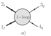
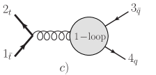
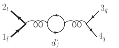
Figure 13: Definition of primitive amplitudes with four quarks. Figure (a) defines $\mathcal{A}_{a}$ which includes all topologies where both external fermion lines enter the loop. Figures (b) and (c) define $\mathcal{A}_{b}$ and $\mathcal{A}_{c}$ where either the top quark or the light quark line enter the loop, respectively. Finally, Figure (d) defines amplitude $\mathcal{A}_{d}$ that includes topologies with a closed fermion loop.

where $\mathcal{A}^{\mathrm{L},[1]}$ and $\mathcal{A}^{\mathrm{L},[1/2]}_{f}$ are regular primitive amplitudes as defined in bdk . The sum over $f$ in Eq.(38) and Eq.(40) includes all quark flavors. The color decomposition of the matrix element for the process $q\bar{q}\rightarrow t\bar{t}\gamma$ follows Ref. egkmz and is given by

$$\mathcal{M}^{\mathrm{virt}}(q\bar{q}\rightarrow t\bar{t}\gamma)=g_{s}^{4}\;\sqrt{2}\,eQ_{t}\!\!\sum_{i=\mathrm{a,b,c,d}} \bigg{[} \delta^{\bar{i}_{1}}_{i_{4}}\delta^{\bar{i}_{3}}_{i_{2}}\mathcal{B}^{\mathrm{virt}}_{1,i}(1_{\bar{t}},2_{t},3_{\bar{q}},4_{q};5_{\gamma})$$ (41)

$$+ \delta^{\bar{i}_{1}}_{i_{2}}\delta^{\bar{i}_{3}}_{i_{4}}\mathcal{B}^{\mathrm{virt}}_{2,i}(1_{\bar{t}},2_{t},3_{\bar{q}},4_{q};5_{\gamma})\bigg{]}$$

with

$$\mathcal{B}^{\mathrm{virt}}_{1,\mathrm{a}}(1_{\bar{t}},2_{t},3_{\bar{q}},4_{q};5_{\gamma}) = \bigg{(}N_{\mathrm{c}}-\frac{2}{N_{\mathrm{c}}}\bigg{)}\bigg{(}\mathcal{A}_{\mathrm{a}}(1_{\bar{t}},5_{g},2_{t},3_{\bar{q}},4_{q})+\frac{Q_{q}}{Q_{t}}\mathcal{A}_{\mathrm{a}}(1_{\bar{t}},2_{t},3_{\bar{q}},5_{g},4_{q})\bigg{)}$$ (42)

$$-\frac{2}{N_{\mathrm{c}}}\bigg{(}\mathcal{A}_{\mathrm{a}}(1_{\bar{t}},5_{g},2_{t},4_{q},3_{\bar{q}})-\frac{Q_{q}}{Q_{t}}\mathcal{A}_{\mathrm{a}}(1_{\bar{t}},2_{t},4_{q},5_{g},3_{\bar{q}})\bigg{)},$$

$$\mathcal{B}^{\mathrm{virt}}_{1,\mathrm{b}}(1_{\bar{t}},2_{t},3_{\bar{q}},4_{q};5_{\gamma}) = -\frac{2\kappa+1}{3N_{\mathrm{c}}}\bigg{(}\mathcal{A}_{\mathrm{b}}(1_{\bar{t}},5_{g},4_{q},3_{\bar{q}},2_{t})+\mathcal{A}_{\mathrm{b}}(1_{\bar{t}},4_{q},5_{g},3_{\bar{q}},2_{t})$$ (43)

$$+\mathcal{A}_{\mathrm{b}}(1_{\bar{t}},4_{q},3_{\bar{q}},5_{g},2_{t})-\frac{Q_{q}}{Q_{t}}\mathcal{A}_{\mathrm{b}}(1_{\bar{t}},4_{q},5_{g},3_{\bar{q}},2_{t})\bigg{)},$$

$$\mathcal{B}^{\mathrm{virt}}_{1,\mathrm{c}}(1_{\bar{t}},2_{t},3_{\bar{q}},4_{q};5_{\gamma}) = -\frac{1}{N_{\mathrm{c}}}\bigg{(}\mathcal{A}_{\mathrm{c}}(1_{\bar{t}},5_{g},2_{t},3_{\bar{q}},4_{q})-\frac{Q_{q}}{Q_{t}}\bigg{\{}\mathcal{A}_{\mathrm{c}}(1_{\bar{t}},2_{t},5_{g},3_{\bar{q}},4_{q})$$ (44)

$$+\mathcal{A}_{\mathrm{c}}(1_{\bar{t}},2_{t},3_{\bar{q}},4_{q},5_{g})+\mathcal{A}_{\mathrm{c}}(1_{\bar{t}},5_{g},2_{t},3_{\bar{q}},4_{q})\bigg{\}}\bigg{)},$$

$$\mathcal{B}^{\mathrm{virt}}_{1,\mathrm{d}}(1_{\bar{t}},2_{t},3_{\bar{q}},4_{q};5_{\gamma}) = \sum_{f}\bigg{(}\mathcal{A}_{\mathrm{d}}^{f}(1_{\bar{t}},5_{g},2_{t},3_{\bar{q}},4_{q})+\frac{Q_{q}}{Q_{t}}\mathcal{A}_{\mathrm{d}}^{f}(1_{\bar{t}},2_{t},3_{\bar{q}},5_{g},4_{q})\bigg{)}.$$ (45)

The primitive amplitudes $\mathcal{A}_{\mathrm{a,b,c,d}}$ correspond to different topologies depending on which fermion lines enter the loop, see Fig. 13. We note that the contribution of the amplitude $B_{2,i}^{\rm virt}$ vanishes after its interference with the tree amplitude is computed; for this reason, we do not present it here.

Appendix B Formula for the production cross-section

In this Appendix, we present the formula that we use to describe radiative corrections to top quark pair production in association with a photon in the narrow width approximation. In the narrow width approximation, the differential production cross-section is given by

$${\rm d}\sigma={\rm d}\sigma_{t\bar{t}\gamma}{\rm d}{\cal B}_{t,X}{\rm d}{\cal B}_{\bar{t},Y}+{\rm d}\sigma_{t\bar{t}}\left[{\rm d}{\cal B}_{t,X\gamma}{\rm d}{\cal B}_{\bar{t},Y}+{\rm d}{\cal B}_{t,X}{\rm d}{\cal B}_{\bar{t},Y\gamma}\right],$$ (46)

where ${\cal B}_{t,X(\gamma)}$ is the branching fraction for either radiative $t\to X+\gamma$ or non-radiative $t\to X$ top quark decay. The above equation is valid to all orders in the strong coupling constant. We expand through ${\cal O}(\alpha_{s}^{3})$ and denote

$${\cal B}_{i,X}^{\rm LO}=\frac{{\rm d}\Gamma^{\rm LO}_{i\to X}}{\Gamma^{\rm LO}_{t}},\;\;\;{\cal B}_{i,X}^{\delta\rm NLO}=\frac{{\rm d}\Gamma^{\delta\rm NLO}_{i\to X}}{\Gamma^{\rm LO}_{t}},\;\;\;\;\;\;\chi=1-2\frac{\Gamma_{t}^{\delta\rm NLO}}{\Gamma_{t}^{\rm LO}},$$ (47)

where $i\in[t,\bar{t}]$, $\Gamma^{\rm LO}_{t}$ is the total decay width of the top quark at leading order and $\Gamma^{\delta\rm LO}_{t}$ is the QCD correction to the total top quark decay width. We obtain

$${\rm d}\sigma = \chi\;\mathrm{d}\sigma^{\mathrm{LO}}_{t\bar{t}}\left(\;\mathrm{d}{\cal B}^{\mathrm{LO}}_{\bar{t},Y\gamma}\;\mathrm{d}{\cal B}^{\mathrm{LO}}_{t,X}+\;\mathrm{d}{\cal B}^{\mathrm{LO}}_{\bar{t},Y}\;\mathrm{d}{\cal B}^{\mathrm{LO}}_{t,X\gamma}\right)+\chi\;\mathrm{d}\sigma^{\mathrm{LO}}_{t\bar{t}\gamma}\;\mathrm{d}{\cal B}^{\mathrm{LO}}_{\bar{t},Y}\;\mathrm{d}{\cal B}^{\mathrm{LO}}_{t,X}$$ (48)

$$+ \;\mathrm{d}\sigma^{\delta\mathrm{NLO}}_{t\bar{t}}\left(\;\mathrm{d}{\cal B}^{\mathrm{LO}}_{\bar{t},Y\gamma}\;\mathrm{d}{\cal B}^{\mathrm{LO}}_{t,X}+\;\mathrm{d}{\cal B}^{\mathrm{LO}}_{\bar{t},Y}\;\mathrm{d}{\cal B}^{\mathrm{LO}}_{t,X\gamma}\right)$$

$$+ \;\mathrm{d}\sigma^{\mathrm{LO}}_{t\bar{t}}\Big{(}\;\mathrm{d}{\cal B}^{\delta\mathrm{NLO}}_{\bar{t},Y\gamma}\;\mathrm{d}{\cal B}^{\mathrm{LO}}_{t,X}+\;\mathrm{d}{\cal B}^{\mathrm{LO}}_{\bar{t},Y}\;\mathrm{d}{\cal B}^{\delta\mathrm{NLO}}_{t,X\gamma}+\;\mathrm{d}{\cal B}^{\delta\mathrm{NLO}}_{\bar{t},Y}\;\mathrm{d}{\cal B}^{\mathrm{LO}}_{t,X\gamma}+\;\mathrm{d}{\cal B}^{\mathrm{LO}}_{\bar{t},Y\gamma}\;\mathrm{d}{\cal B}^{\delta\mathrm{NLO}}_{t,X}\Big{)}$$

$$+ \;\mathrm{d}\sigma^{\delta\mathrm{NLO}}_{t\bar{t}\gamma}\;\mathrm{d}{\cal B}^{\mathrm{LO}}_{\bar{t},Y}\;\mathrm{d}{\cal B}^{\mathrm{LO}}_{t,X}+\;\mathrm{d}\sigma^{\mathrm{LO}}_{t\bar{t}\gamma}\left(\;\mathrm{d}{\cal B}^{\delta\mathrm{NLO}}_{\bar{t},Y}\;\mathrm{d}{\cal B}^{\mathrm{LO}}_{t,X}+\;\mathrm{d}{\cal B}^{\mathrm{LO}}_{\bar{t},Y}\;\mathrm{d}{\cal B}^{\delta\mathrm{NLO}}_{t,X}\right)+{\cal O}(\alpha_{s}^{4}).$$

Since we also treat the $W$-boson in the narrow width approximation, photon radiation in the top quark decay can be further decomposed into photon radiation in top quark ($t\to Wb$) and $W$ ($W\to f\bar{f}^{\prime}$) decays. The decays of the $W$-bosons are treated at leading order in perturbative QCD. We therefore write

$${\rm d}{\cal B}_{t,X\gamma}^{i}=\frac{\mathrm{d}\Gamma_{bW\gamma}^{i}}{\Gamma^{\mathrm{LO}}_{t}}\;\frac{\mathrm{d}\tilde{\Gamma}_{W\to f\bar{f^{\prime}}}^{\text{LO}}}{\Gamma_{W}}+\frac{\mathrm{d}\Gamma_{bW}^{i}}{{\Gamma^{\mathrm{LO}}_{t}}}\;\frac{\mathrm{d}\tilde{\Gamma}_{W\to f\bar{f^{\prime}}\gamma}^{\text{LO}}}{\Gamma_{W}},\;\;\;\;i\in[{\rm LO},\delta{\rm NLO}],\;\;X=bf\bar{f}^{\prime}.$$ (49)

References

- (1) V.M. Abazov et al. [D0 Collaboration], Phys. Rev. Lett. 98, 041801 (2007).
- (2) D. Chang, W.F. Chang and E. Ma, Phys. Rev. D59, 091503 (1999).
- (3) U. Baur, M. Buice, L. H. Orr, Phys. Rev. D64, 094019 (2001).
- (4) T. Aaltonen et al. [CDF Collaboration], Phys. Rev. D80, 011102(R) (2009).
- (5) B. Auerbach and H. Frisch, private communication.
- (6) U. Baur, A. Juste and L.H. Orr, D. Rainwater, Phys. Rev. D71, 054013 (2005).
- (7) Peng-Fei Duan, Wen-Gan Ma, Ren-You Zhang, Liang Han, Lei Guo, Shao-Ming Wang, Phys. Rev. D80, 014022 (2009).
- (8) W. T. Giele, Z. Kunszt and K. Melnikov, JHEP 0804, 049 (2008).
- (9) R. K. Ellis, W. T. Giele, Z. Kunszt, K. Melnikov, Nucl. Phys. B 822, 270 (2009).
- (10) K. Melnikov and M. Schulze, JHEP 0908:049 (2009).
- (11) K. Melnikov and M. Schulze, Nucl. Phys. B 840, 129 (2010).
- (12) V.S. Fadin, V.A. Khoze and A.D. Martin, Phys. Rev. D 49, 2247 (1994); K. Melnikov and O.I. Yakovlev, Phys. Lett. B 324, 217 (1994); K. Melnikov and O.I. Yakovlev, Nucl. Phys. B 471, 90 (1996).
- (13) G. Bevilacqua, M. Czakon, A. van Hameren et al., [arXiv:1012.4230 [hep-ph]].
- (14) A. Denner, S. Dittmaier, S. Kallweit et al., [arXiv:1012.3975 [hep-ph]].
- (15) W. Beenakker, S. Dittmaier, M. Kramer et al., Nucl. Phys. B653, 151-203 (2003).
- (16) S. Dawson, C. Jackson, L. H. Orr et al., Phys. Rev. D68, 034022 (2003).
- (17) A. Lazopoulos, T. McElmurry, K. Melnikov et al., Phys. Lett. B666, 62-65 (2008).
- (18) S. Dittmaier, P. Uwer and S. Weinzierl, Phys. Rev. Lett. 98, 262002 (2007).
- (19) S. Dittmaier, P. Uwer and S. Weinzierl, Eur. Phys. J. C 59, 625 (2009).
- (20) G. Bevilacqua, M. Czakon, C. G. Papadopoulos et al., Phys. Rev. Lett. 104, 162002 (2010).
- (21) A. Bredenstein, A. Denner, S. Dittmaier et al., JHEP 0808, 108 (2008).
- (22) A. Bredenstein, A. Denner, S. Dittmaier et al., Phys. Rev. Lett. 103, 012002 (2009).
- (23) G. Bevilacqua, M. Czakon, C. G. Papadopoulos et al., JHEP 0909, 109 (2009).
- (24) A. Bredenstein, A. Denner, S. Dittmaier et al., JHEP 1003, 021 (2010).
- (25) A. Kardos, C. Papadopoulos, Z. Trocsanyi, [arXiv:1101.2672 [hep-ph]].
- (26) Z. Bern, L. Dixon and D. Kosower, Nucl. Phys. B437, 259 (1995).
- (27) G. Ossola, C. G. Papadopoulos and R. Pittau, Nucl. Phys. B 763, 147 (2007).
- (28) T. Hahn, Comput. Phys. Commun. 140, 418 (2001).
- (29) S. Catani and M. H. Seymour, Nucl. Phys. B 485, 291 (1997) [Erratum-ibid. B 510, 503 (1998)].
- (30) S. Catani, S. Dittmaier, M. H. Seymour and Z. Trocsanyi, Nucl. Phys. B 627, 189 (2002).
- (31) J. M. Campbell and R.K. Ellis, Phys. Rev. D 62, 114012 (2000). The MCFM program is publicly available from http://mcfm.fnal.gov.
- (32) J. M. Campbell and F. Tramontano, Nucl. Phys. B 726, 109 (2005).
- (33) Z. Nagy and Z. Trócsányi, Phys. Rev. Lett. 87, 082001 (2001), Z. Nagy, Phys. Rev. D 68, 094002 (2003).
- (34) J. Pumplin, D. R. Stump, J. Huston, H. L. Lai, P. M. Nadolsky and W. K. Tung, JHEP 0207, 012 (2002).
- (35) P. M. Nadolsky et al., Phys. Rev. D 78, 013004 (2008).
- (36) S. Frixione, Phys. Lett. B429, 369-374 (1998).
- (37) J. H. Kühn and G. Rodrigo, Phys. Rev. D 59, 054017 (1999); Phys. Rev. Lett. 81, 49 (1998).
- (38) G. Passarino and and M. Veltman, Nucl. Phys. B160, 151 (1979).
- (39) J. M. Campbell, R. K. Ellis and F. Tramontano, Phys. Rev. D 70, 094012 (2004).
- (40) M. Jezabek and J. H. Kühn, Nucl. Phys. B314, 1 (1989).
- (41) S. Catani, Y.L. Dokshitzer, M. H. Seymour and B.R. Webber, Nucl. Phys. B406, 187 (1993).
- (42) S.D. Ellis and D. E. Soper, Phys. Rev. D48, 3160 (1993).
- (43) W. Bernreuther, J. Phys. G 35, 083001 (2008).
- (44) Z. Bern, L. Dixon and D. Kosower, Ann. Rev. Nucl. Part. Sci. 46, 109 (1996).
- (45) R. K. Ellis, W. T. Giele, Z. Kunszt, K. Melnikov and G. Zanderighi, JHEP 0901, 012 (2009).