Phase diagram of the lattice $G_{2}$ Higgs Model

Abstract

We study the phases and phase transition lines of the finite temperature $G_{2}$ Higgs model. Our work is based on an efficient local hybrid Monte-Carlo algorithm which allows for accurate measurements of expectation values, histograms and susceptibilities. On smaller lattices we calculate the phase diagram in terms of the inverse gauge coupling $\beta$ and the hopping parameter $\kappa$. For $\kappa\to 0$ the model reduces to $G_{2}$ gluodynamics and for $\kappa\to\infty$ to $SU(3)$ gluodynamics. In both limits the system shows a first order confinement-deconfinement transition. We show that the first order transitions at asymptotic values of the hopping parameter are almost joined by a line of first order transitions. A careful analysis reveals that there exists a small gap in the line where the first order transitions turn into continuous transitions or a cross-over region. For $\beta\to\infty$ the gauge degrees of freedom are frozen and one finds a nonlinear $O(7)$ sigma model which exhibits a second order transition from a massive $O(7)$-symmetric to a massless $O(6)$-symmetric phase. The corresponding second order line for large $\beta$ remains second order for intermediate $\beta$ until it comes close to the gap between the two first order lines. Besides this second order line and the first order confinement-deconfinement transitions we find a line of monopole-driven bulk transitions which do not interfer with the confinement-deconfinment transitions.

I Introduction

Quarks and gluons are confined in mesons and baryons and are not seen as asymptotic states of strong interaction. Understanding the dynamics of this confinement mechanism is one of the challenging problems in strongly coupled gauge theories. Confinement is lost under extreme conditions: when temperature reaches the QCD energy scale or the density rises to the point where the average inter-quark separation is less than $1$ fm, then hadrons are melted into their constituent quarks.

For gauge groups with a non-trivial center is the Polyakov loop

$$P(\vec{x})=\operatorname{tr}\mathcal{P}(\vec{x}),\quad\mathcal{P}(\vec{x})=\frac{1}{N}\operatorname{tr}\left(\exp\;i\int_{0}^{\beta_{T}}A_{0}(\tau,\vec{x})\,d\tau\right),\quad\beta_{T}=\frac{1}{kT},$$ (1)

an order parameter for the transition from the confined to the unconfined phase in gluodynamics (pure gauge theories). Its thermal expectation value is related to the difference in free energy $F$ due to the presence of an infinitely heavy test quark in the gluonic bath as

$$\langle P\rangle\propto e^{-\beta F},$$ (2)

such that $\langle P\rangle\neq 0$ in the unconfined high-temperature phase and $\langle P\rangle=0$ in the confined low-temperature phase. Below the critical temperature is $\mathcal{P}(\vec{x})$ uniformly distributed over the group manifold and above the critical temperature it is in the neighborhood of a center-element. Near the transition point its dynamics is successfully described by effective three dimensional scalar field models for the characters of $\mathcal{P}(\vec{x})$ Svetitsky:1982gs ; Yaffe:1982qf ; Wozar:2006fi . If one further projects the Polyakov loops onto the center of the gauge group, then one arrives at generalized Potts models describing the effective Polyakov-loop dynamics wipf:2006wj .

With matter in the fundamental representation the center symmetry is explicitly broken and for all temperatures has $P$ a non-zero expectation value and points in the direction of a particular center element. Thus in the strict sense the Polyakov loop ceases to be an order parameter for the center symmetry. On a microscopic scale this is attributed to the breaking of the string connecting a static ‘quark anti-quark pair’ when one tries to separate the static charges Greensite:2003bk . It breaks via the spontaneous creation of dynamical quark anti-quark pairs which in turn screen the individual static charges.

To clarify the relevance of the center symmetry for confinement it suggests itself to study gauge theories for which the gauge group has a trivial center. Then the Polyakov loop ceases to be an order parameter even in the absence of dynamical matter since the strings connecting external charges can break via the spontaneous creation of dynamical ‘gluons’. The smallest simple and simply connected Lie group with a trivial center is the $14$ dimensional exceptional Lie group $G_{2}$. This is one reason why $G_{2}$ gauge theory with and without Higgsfields has been investigated in series of papers Holland:2003kg ; Holland:2003jy ; Pepe:2006er ; Greensite:2006sm ; Danzer:2008bk ; Maas:2007af . Although there is no symmetry reason for a deconfinement phase transition in $G_{2}$ gluodynamics it has been conjectured that a first order deconfinement transition without order parameter exists. In this context confinement refers to confinement at intermediate scales, where a Casimir scaling of string tensions has been detected in Liptak:2008gx . Although the threshold energy for string breaking in $G_{2}$ gauge theory is rather high, string breaking has been seen in $3$ dimensional $G_{2}$ gluodynamics in Wellegehausen:2010ai .

The gauge group $SU(3)$ of strong interaction is a subgroup of $G_{2}$ and this observation has interesting consequences, as pointed out in Holland:2003jy . With a Higgs field in the fundamental $7$ dimensional representation one can break the $G_{2}$ gauge symmetry to the $SU(3)$ symmetry via the Higgs mechanism. When the Higgs field in the action

$$S[A,\phi]=\int d^{4}x\left(\frac{1}{4g^{2}}\operatorname{tr}F_{\mu\nu}F^{\mu\nu}+\frac{1}{2}(D_{\mu}\phi,D_{\mu}\phi)+V(\phi)\right)$$ (3)

picks up a vacuum expectation value $v$, then $6$ gauge bosons acquire a mass proportional to $v$ while the $8$ gluons belonging to $SU(3)$ remain massless. The massive gauge bosons are removed from the spectrum for $v\to\infty$. In this limit $G_{2}$ Higgs model reduces to $SU(3)$ Yang-Mills theory. Even more interesting, for intermediate and large values of $v$ the $G_{2}$ Yang-Mills-Higgs (YMH) theory mimics $SU(3)$ gauge theory with dynamical ‘scalar quarks’. The masses of these ‘quarks’ and the length scale at which string breaking occurs increase with increasing $v$. The Polyakov loop serves as approximate order parameter separating the confined from the unconfined phases with a rapid change at the transition or crossover. This rapid change is depicted in Fig. 1 which shows the expectation value of $P$ for $G_{2}$ gluodynamics as function of the inverse gauge coupling $\beta=1/g^{2}$.

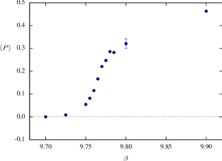
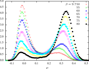
Figure 1: Phase transition on a $16^{3}\times 6$ lattice in terms of the Polyakov loop in the fundamental representation of $G_{2}$. The rapid change of the Polyakov loop with $\beta=1/g^{2}$ (left panel) and histograms of the Polyakov loop for $\beta$ in the vicinity of $\beta_{c}$ (right panel) point to a first order transition.

In an earlier work we derived a $3$ dimensional effective theory for the dynamics of the Polyakov loop for finite temperature $G_{2}$ gluodynamics and analyzed the resulting Landau-type theory with the help of elaborate Monte Carlo simulations Wellegehausen:2009rq . Already the leading order effective Polyakov loop model exhibits a rich phase structure with symmetric, ferromagnetic, and anti-ferromagnetic phases.

In the present paper we investigate the phase structure of microscopic $G_{2}$ YMH lattice theory with a Higgs field in the $7$ dimensional representation. The corresponding lattice action for the $G_{2}$ valued link variables and a normalized Higgs field with $7$ real components reads

$$S_{\rm YMH}[\,\mathcal{U},\Phi]=\beta\sum\limits_{\square}\left(1-\frac{1}{7}\operatorname{tr}\operatorname{Re}\mathcal{U}_{\square}\right)-\kappa\sum\limits_{x,\mu}\Phi_{x+\hat{\mu}}\,\mathcal{U}_{x,\mu}\Phi_{x},\quad\Phi_{x}\cdot\Phi_{x}=1,$$ (4)

and depends on the inverse gauge coupling $\beta$ and the hopping parameter $\kappa$. For $\beta\to\infty$ the gauge bosons decouple and the theory reduces to an $O(7)$ invariant nonlinear sigma model which is expected the have a second order (mean field) symmetry breaking transition down to $O(6)$. The mean field prediction for the critical coupling is $\kappa_{c,\rm mf}=7/8$ and this value bounds $\kappa_{c}$ from below simon80 . In the limit $\kappa=0$ we recover $G_{2}$ gluodynamics with a first order deconfinement phase transition, in agreement with the findings in Cossu:2008 . In the other extreme case $\kappa\to\infty$ we end up with $SU(3)$ gluodynamics with a weak first order deconfinement transition. The known transitions in the limiting cases $\kappa\to 0,\;\kappa\to\infty$ or $\beta\to\infty$ are depicted in Fig. 2.

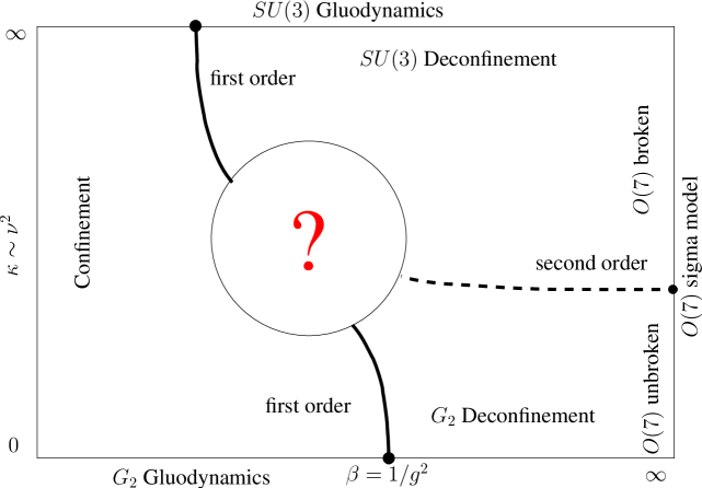
Figure 2: Expected phase diagram in the parameter space $(1/g^{2},\kappa)$ (taken from Pepe:2006er ).

If $\kappa$ is lowered from $\infty$ then in addition to the $8$ gluons of $SU(3)$, the $6$ additional gauge bosons of $G_{2}$ with decreasing mass begin to participate in the dynamics. Similarly as dynamical quarks and anti-quarks, they transform in the representations $\{3\}$ and $\{\bar{3}\}$ of $SU(3)$ and thus explicitly break the $\mathbb{Z}_{3}$ center symmetry. As in QCD they are expected to weaken the deconfinement phase transition. Thus it has been conjectured in Pepe:2006er that there may exist a critical endpoint where the transition disappears.

In the following section we shall briefly recall those facts about $G_{2}$ representations which are relevant for the present work. In Sec. III some algorithmic aspects are reviewed. A more detailed presentation can be found in our earlier paper Wellegehausen:2010ai . Sec. IV contains our Monte-Carlo results for the phase diagram in the $(\beta,\kappa)$ plane. We find that the two first order lines emanating from the deconfinement transitons in $G_{2}$ and $SU(3)$ gluodynamics at $\kappa=0$ and $\kappa=\infty$ end in the vicinity of $(\beta,\kappa)=(9.4,1.6)$ on a $6\times 16^{3}$ lattice. Sec. VI contains the results of our high statistics simulations for histograms and susceptibilities in the small region in parameter space where the two first order lines are either connected by a second order line or leave open a gap which smoothly connects the confinend and deconfined phases. Our data are consistent with the conjectured critical endpoints attached to the two first order lines. For large $\beta$ a second order transition line which separates the $O(7)$ and $O(6)$ sigma models comes close to the first order deconfinement transition lines. The phases and transition lines are localized and analysed with high statistics simulations of the Polyakov loop distribution and susceptibility, plaquette and Higgs action susceptibilities, and finally with derivatives of the mean action with respect to the hopping parameter. Besides the transition lines indicated in Fig. 2 there exists another line of monopole driven bulk transitions. This line emanates from the bulk crossover in pure $G_{2}$-gluodynamics at $\beta=9.45$ Cossu:2008 .

II The group $\bm{G_{2}}$

The exceptional Lie group $G_{2}$ is the smallest Lie group in the Cartan classification which is simply connected and has a trivial center. The two fundamental representations are the $7$ dimensional defining representation $\{7\}$ and the $14$ dimensional adjoint representation $\{14\}$. One may view the elements of the representation $\{7\}$ as matrices in the defining representation of $SO(7)$, subject to seven independent cubic constraints, see Holland:2003jy . For example, the defining representation $\{7\}$ of $SO(7)$ turns into an irreducible representation of $G_{2}$, whereas the adjoint representation $\{21\}$ of $SO(7)$ branches into the two fundamental representation $\{14\}$ and $\{7\}$ of $G_{2}$. The gauge group of strong interaction is a subgroup of $G_{2}$ and the corresponding coset space is a sphere Macfarlane:2002hr ,

$$G_{2}/SU(3)\sim S^{6}.$$ (5)

This means that every element $\mathcal{U}$ of $G_{2}$ can be written as

$$\mathcal{U}=\mathcal{S}\cdot\mathcal{V}\quad\text{with}\quad\mathcal{S}\in G_{2}/SU(3)\quad\text{and}\quad\mathcal{V}\in SU(3),$$ (6)

and we shall use this decomposition to speed up our numerical simulations.

Quarks in $G_{2}$ transform under the $7$ dimensional fundamental representation, gluons under the $14$ dimensional fundamental (and adjoint) representation. To better understand $G_{2}$ gluodynamics we recall the decomposition of tensor products

$$\{7\}\otimes\{7\} =\{1\}\oplus\{7\}\oplus\{14\}\oplus\{27\},$$ (7)

$$\{7\}\otimes\{7\}\otimes\{7\} =\{1\}\oplus 4\cdot\{7\}\oplus 2\cdot\{14\}\oplus 3\cdot\{27\}\oplus 2\cdot\{64\}\oplus\{77^{\prime}\},$$

$$\{14\}\otimes\{14\} =\{1\}\oplus\{14\}\oplus\{27\}\oplus\{77\}\oplus\{77^{\prime}\},$$

$$\{14\}\otimes\{14\}\otimes\{14\} =\{1\}\oplus\{7\}\oplus 5\cdot\{14\}\oplus 3\cdot\{27\}\oplus\dotsb.$$

These decompositions show similarlies to QCD: two quarks, three quarks, two gluons and three gluons can build colour singlets – mesons, baryons and glueballs. In $G_{2}$ gauge theory three gluons can screen the colour charge of a single quark,

$$\{7\}\otimes\{14\}\otimes\{14\}\otimes\{14\}=\{1\}\oplus\dotsb,$$ (8)

and this explains why the string between two external charges in the $\{7\}$ representation will break for large charge separations. The two remnants are colour blind glue lumps. The same happens for two external charges in the adjoint representation. In a previous work we did observe string breaking at the expected separation between the two charges Wellegehausen:2010ai .

The $G_{2}$ gauge symmetry can be broken to $SU(3)$ with the help of a Higgs field in the $7$ dimensional representation. For $\kappa\to\infty$ the factor $\mathcal{S}$ in the decomposition (6) is frozen and we end up with an $SU(3)$ gauge theory with rescaled gauge coupling for the factor $\mathcal{U}$. With respect to the unbroken subgroup $SU(3)$ the fundamental representations $\{7\}$ and $\{14\}$ branch into the following irreducible $SU(3)$ representations:

$$\{7\} \longrightarrow\{3\}\oplus\{\bar{3}\}\oplus\{1\},$$ (9)

$$\{14\} \longrightarrow\{8\}\oplus\{3\}\oplus\{\bar{3}\}.$$

The Higgs field branches into a scalar quark, scalar anti-quark and singlet with respect to $SU(3)$. Similarly, the $G_{2}$ gluons branch into massless $SU(3)$ gluons and additional gauge bosons with respect to $SU(3)$. The latter eat up the non-singlet scalar fields such that the spectrum in the broken phase consists of $8$ massless gluons, $6$ massive gauge bosons and one massive Higgs particle.

III Algorithmic considerations

III.1 Equations of motion for local hybrid Monte-Carlo

In this work we employ a local version of the hybrid Monte-Carlo (HMC) algorithm where single site and link variables are evolved in a HMC style Marenzoni:1993im . The algorithm assumes a local interaction and hence applies to all purely bosonic theories. The implementation for the $G_{2}$ Higgs model is a mild generalization of the algorithm used in our previous work on $G_{2}$ gluodynamics Wellegehausen:2010ai . We use a local hybrid Monte-Carlo (LHMC) algorithm for several good reasons: First there is no low Metropolis acceptance rate even for large hopping parameters. More precisely, in a heat bath algorithm combined with an over-relaxation we would need two Metropolis steps in each update for $\kappa>0$ which for large $\kappa$ may lead to low acceptance rates. With the LHMC-algorithm we can avoid this problem and deal with arbitrary values of $\kappa$. Autocorrelation times can be controlled (in certain ranges) by the integration time in the molecular dynamics part of the HMC algorithm. Second, the formulation is given entirely in terms of Lie group and Lie algebra elements and there is no need to back-project onto the group. For $G_{2}$ it is possible to use a real representation and in addition an analytical expression for the involved exponential maps from the algebra to the group. These maps allow for a fast implementation of the LHMC algorithm.

This algorithm has been essential for obtaining the accurate results in the present work. Since we developed and used the first implementation for $G_{2}$ it may be useful to sketch how it works for this exceptional group. More details can be found in Wellegehausen:2010ai . For $G_{2}$ YMH lattice theory the (L)HMC algorithm is based on a fictitious dynamics for the link-variables on the $G_{2}$ manifold and the normalized Higgs field on the $6$-sphere. The “free evolution” on a semisimple group is the Riemannian geodesic motion with respect to the Cartan-Killing metric

$$ds^{2}_{G}=\kappa\operatorname{tr}\left(d\mathcal{U}\mathcal{U}^{-1}\otimes d\mathcal{U}\mathcal{U}^{-1}\right).$$ (10)

In a (L)HMC dynamics the interaction term is given by the YMH action (4) of the underlying lattice gauge theory and hence it is natural to derive the HMC dynamics from a Lagrangian of the form

$$L_{\rm HMC}=-\frac{1}{2}\sum\limits_{x,\mu}\operatorname{tr}\left(\dot{\mathcal{U}}_{x,\mu}\mathcal{U}_{x,\mu}^{-1}\right)^{2}+K(\Phi,\dot{\Phi})-S_{\text{YMH}}[\,\mathcal{U},\Phi],$$ (11)

where ‘dot’ denotes the derivative with respect to the fictitious time parameter $\tau$ and $K(\Phi,\dot{\Phi})$ is a kinetic term for the Higgs field. To update the normalized Higgs field we set

$$\Phi_{x}=\mathcal{O}_{x}\Phi_{0}\quad\hbox{with}\quad\mathcal{O}_{x}\in SO(7)$$ (12)

and constant $\Phi_{0}$. The change of variables $\Phi_{x}\to\mathcal{O}_{x}$ converts the induced measure on $S^{6}\subset R^{7}$ into the Haar measure of $SO(7)$. Without interaction the rotation matrices $\mathcal{O}_{x}$ will evolve freely on the group manifold $SO(7)$ such that in terms of the $(\mathcal{U},\mathcal{O})$ variables we choose as Lagrangian for the HMC dynamics

$$L=-\frac{1}{2}\sum\limits_{x,\mu}\operatorname{tr}\left(\dot{\mathcal{U}}_{x,\mu}\mathcal{U}_{x,\mu}^{-1}\right)^{2}-\frac{1}{2}\sum\limits_{x}\operatorname{tr}\left(\dot{\mathcal{O}}_{x}\mathcal{O}^{-1}_{x}\right)^{2}-S_{\rm YMH}[\,\mathcal{U},\mathcal{O}]\,.$$ (13)

The Lie algebra valued fictitious momenta conjugated to the link variable $\mathcal{U}_{x,\mu}$ and site variable $\mathcal{O}_{x}$ are given by

$$\mathfrak{P}_{x,\mu}=\frac{\partial L}{\partial\big{(}\dot{\mathcal{U}}_{x,\mu}\mathcal{U}_{x,\mu}^{-1}\big{)}}=-\dot{\mathcal{U}}_{x,\mu}\mathcal{U}_{x,\mu}^{-1}\quad,\quad\mathfrak{Q}_{x}=\frac{\partial L}{\partial\big{(}\dot{\mathcal{O}}_{x}\mathcal{O}_{x}^{-1}\big{)}}=-\dot{\mathcal{O}}_{x}\mathcal{O}_{x}^{-1}.$$ (14)

The Legendre transform yields the following pseudo-Hamiltonian

$$H=-\frac{1}{2}\sum_{x,\mu}\operatorname{tr}\mathfrak{P}_{x,\mu}^{2}-\frac{1}{2}\sum_{x}\operatorname{tr}\mathfrak{Q}_{x}^{2}+S_{\text{YMH}}[\,\mathcal{U},\mathcal{O}].$$ (15)

Note that for real $\mathcal{U}_{x,\mu}$ and $\mathcal{O}_{x}$ the momenta are antisymmetric such that both kinetic terms are positive. The equations of motion for the momenta are obtained by varying the Hamiltonian. The variation of $S_{\text{\rm YMH}}[\,\mathcal{U},\mathcal{O}]$ with respect to a fixed link variable $\mathcal{U}_{x,\mu}$ yields the staple variable $R_{x,\mu}$, the sum of triple products of elementary link variables closing to a plaquette with the chosen link variable. Setting

$$\delta\mathfrak{P}_{x,\mu}=\dot{\mathfrak{P}}_{x,\mu}d\tau,\quad\delta\mathcal{U}_{x,\mu}=\dot{\mathcal{U}}_{x,\mu}d\tau=-\mathfrak{P}_{x,\mu}\mathcal{U}_{x,\mu}d\tau$$ (16)

with similar expressions for the momentum and field variables $\mathfrak{Q}_{x}$ and $\mathcal{O}_{x}$ in the Higgs sector yields for the variation of the HMC Hamiltonian

$$\delta H=-\sum\limits_{x,\mu}\operatorname{tr}\mathfrak{P}_{x,\mu}\big{\{}\dot{\mathfrak{P}}_{x,\mu}-F_{x,\mu}\big{\}}-\sum_{x}\operatorname{tr}\mathfrak{Q}_{x}\big{\{}\dot{\mathfrak{Q}}_{x}-G_{x}\big{\}}$$ (17)

with the following “forces” in the gauge and Higgs sector

$$F_{x,\mu}=\frac{\beta}{14}\left(\mathcal{U}_{x,\mu}R_{x,\mu}-R_{x,\mu}^{\dagger}\mathcal{U}^{\dagger}_{x,\mu}\right)+\kappa(\mathcal{U}_{x,\mu}\phi_{x})\phi^{\mathsf{T}}_{x+\mu},\quad G_{x}=\kappa\phi_{x}\Big{(}\sum\nolimits_{y:x}\mathcal{U}_{xy}\,\phi_{y}\Big{)}^{\mathsf{T}},$$ (18)

where the last sum extends over all nearest neighbors $y$ of $x$ and $U_{xy}$ denotes the parallel transporter from $y$ to $x$. The variational principle implies that the projection of the terms between curly brackets onto the Lie algebras $\mathfrak{g}_{2}$ and $\mathfrak{so}(7)$ vanish,

$$\dot{\mathfrak{P}}_{x,\mu}=F_{\mu,x}\big{|}_{\mathfrak{g}_{2}}\quad,\quad\dot{\mathfrak{Q}}_{x}=G_{x}\big{|}_{\mathfrak{so}(7)}.$$ (19)

The equations (14) and (19) determine the fictitious dynamics of the lattice fields in the (L)HMC algorithm. Choosing a trace-orthonormal basis $\{T_{a}\}$ of $\mathfrak{g}_{2}$ the LHMC equations in the gauge sector read

$$\dot{\mathcal{U}}_{x,\mu}=-\mathfrak{P}_{x,\mu}\mathcal{U}_{x,\mu}\quad\hbox{and}\quad\dot{\mathfrak{P}}_{x,\mu}=\sum\limits_{a}\operatorname{tr}\left(F_{x,\mu}T_{a}\right)T_{a}$$ (20)

with force $F_{x,\mu}$ defined in (18). In the Higgs sector they take the form

$$\dot{\mathcal{O}}_{x}=-\mathfrak{Q}_{x}\mathcal{O}_{x}\quad\text{and}\quad\dot{\mathfrak{Q}}_{x}=\sum\limits_{b}\operatorname{tr}\left(G_{x}\tilde{T}_{b}\right)\tilde{T}_{b}$$ (21)

with trace-orthonormal basis $\{\tilde{T}_{b}\}$ of $\mathfrak{so}(7)$ and force $G_{x}$ defined in (18).

III.2 Numerical solutions of YMH-dynamics

We employ a time reversible leap frog integrator which uses the integration scheme

$$\mathfrak{P}_{x,\mu}(\tau+{\textstyle\frac{1}{2}}\delta\tau) =\mathfrak{P}_{x,\mu}(\tau)+{\textstyle\frac{1}{2}}\delta\tau\,\dot{\mathfrak{P}}_{x,\mu}(\tau)$$ (22)

$$\mathcal{U}_{x,\mu}(\tau+\delta\tau) =\exp\left\{-\delta\tau\,\mathfrak{P}_{x,\mu}(\tau+{\textstyle\frac{1}{2}}\delta\tau)\right\}\mathcal{U}_{x,\mu}(\tau)$$

$$\mathfrak{P}_{x,\mu}(\tau+\delta\tau) =\mathfrak{P}_{x,\mu}(\tau+{\textstyle\frac{1}{2}}\delta\tau)+{\textstyle\frac{1}{2}}\delta\tau\,\dot{\mathfrak{P}}_{x,\mu}(\tau+\delta\tau),$$

and similarly for the variables $(\mathcal{O}_{x},\mathfrak{Q}_{x})$ in the Higgs sector. The ‘time’ derivative of $\mathfrak{P}(\tau+\delta\tau)$ in the last step is given in terms of the already known group valued field at $\tau+\delta\tau$ via the equations of motion. Clearly, to calculate $\mathcal{U}$ and $\mathcal{O}$ at time $\tau+\delta\tau$ a fast implementation of exponential maps is required. In the Higgs sector the map $\mathfrak{so}(7)\to SO(7)$ is computed via the Cayley-Hamilton theorem. For small values of the hopping parameter $\kappa$ the step size and integration length for the integration may be chosen as in the gauge field integrator. For an efficient and fast computation of the exponential map $\mathfrak{g}_{2}\to G_{2}$ we exploit the real embedding $\mathcal{V}$ of the representation $3\oplus\bar{3}$ of $SU(3)$ into $G_{2}$,

$$\mathcal{U}=\mathcal{S}\cdot\mathcal{V}(\mathcal{W})\quad\text{with}\quad\mathcal{S}\in G_{2}/SU(3),\quad\mathcal{W}\in SU(3).$$ (23)

For a given time step $\delta\tau$ the factorization will be expressed in terms of the Lie algebra elements with the help of the exponential maps,

$$\exp\left\{\delta\tau\,\mathfrak{u}\right\}=\exp\left\{\delta\tau\,\mathfrak{s}\right\}\cdot\exp\left\{\delta\tau\,\mathfrak{v}\right\}\quad\text{with generators}\quad\mathfrak{u}\in\mathfrak{g}_{2},\;\;\mathfrak{v}\in\mathcal{V}_{*}(\mathfrak{su}(3)).$$ (24)

The exponential maps for the two factors can be calculated efficiently, see Wellegehausen:2010ai . But in the numerical integration we need the exponential map for elements $\mathfrak{u}\in\mathfrak{g}_{2}$. These elements are related to the generators $\mathfrak{s}$ and $\mathfrak{v}$ used in the factorization by the Baker-Campbell-Hausdorff formula,

$$\delta\tau\,\mathfrak{u}=\delta\tau\left(\mathfrak{s}+\mathfrak{v}\right)+\frac{1}{2}\delta\tau^{2}\left[\,\mathfrak{s},\mathfrak{v}\,\right]+\cdots.$$ (25)

For a second order integrator the approximation (25) may be used in the exponentiations needed to calculate $\mathcal{V}$ and $\mathcal{S}$. This approximation leads to a violation of energy conservation which is of the same order as the violation one finds with a second order integrator. To sum up, a LHMC sweep consists of the following steps:

1. Gaussian draw for the momentum variables on a given site and link,

2. Integration of the equations of motion for the given site and link,

3. Metropolis accept/reject step,

4. Repeat these steps for all sites and links of the lattice.

This local version of the HMC does not suffer from an extensive $\delta H\propto V$ problem such that already a second order symplectic (leap frog) integrator allows for sufficiently large time steps $\delta\tau$. For a large range of couplings $(\beta,\kappa)$ in our simulations an integration length of $T=0.75$ with a step size of $\delta\tau=0.25$ is optimal for minimal autocorrelation times and a small number of thermalisation sweeps. Acceptance rates of more than $99\%$ are reached. To compare the performances of our LHMC algorithm with the usually used heat-bath algorithm we estimated the computation time of the different parts in the LHMC-algorithm in units given by the average computation time for one staple in $\Delta S_{\mathcal{U}}$. On an Intel Corei7 CPU the latter is approximately $4\,\mu\text{s}$ for a $12^{3}\times 6$ lattice.

In Table 1 we listed the times needed to change the gauge or Higgs action during a single update of one link or one Higgs field variable, the time for both integrators without exponential map and separately the computation time for a single exponential map. Most time is spent with calculating the exponential maps for $SO(7)$.

Part	$\Delta S_{\mathcal{U}}$	$\Delta S_{\mathcal{O}}$	integr. $\mathcal{U}$	integr. $\mathcal{O}$	exp($G_{2}$)	exp($SO_{7}$)
pure gauge	$1.00$	-	$1.34$	-	$0.42$	-
gauge Higgs	$1.03$	$0.43$	$1.74$	$1.00$	$0.40$	$4.97$

Table 1: Computation times normalized to $\Delta S_{\mathcal{U}}$ (staple).

Note that during the calculation of one exponential map for $SO(7)$ the CPU calculates about $10$ exponential maps for $G_{2}$. Table 2 compares the total time-contributions to one configuration with those of the heat-bath algorithm with overrelaxation. We see that for pure gauge theories the standard heat-bath algorithm with overrelaxation is only two times faster as the LHMC algorithm.

Part	$\Delta S_{\mathcal{U}}$	$\Delta S_{\mathcal{O}}$	integr. $\mathcal{U}$	integr. $\mathcal{O}$	exp($G_{2}$)	exp($SO_{7}$)	$\text{total time}/V\cdot d\cdot\text{Config.}$	heat-bath
pure gauge	$1.00$	-	$1.34$	-	$1.26$	-	$3.60$	$\approx 2$
gauge Higgs	$1.03$	$0.11$	$1.74$	$0.25$	$1.20$	$3.72$	$8.05$	-

Table 2: Total time contribution to one LHMC configuration compared to heat-bath algorithm.

IV The phase diagram of the $G_{2}$ Higgs model: overview

With the help of the local HMC algorithm sketched previously we calculated several relevant observables to probe the phases and phase transition lines in the $(\beta,\kappa)$ plane. First we present the phase diagram obtained on small lattices. For vanishing $\kappa$ we are dealing with $G_{2}$ gluodynamics which shows a first order finite temperature deconfinement phase transition. The transition is discontinuous since there is a large mismatch of degrees of freedom in the confined and unconfined phases. At the other extreme value $\kappa=\infty$ six of the fourteen gauge bosons decouple from the dynamics and we are left with $SU(3)$ gluodynamics, which shows a first order deconfinement phase transition as well. The question arises whether the first order transitions in $G_{2}$ and $SU(3)$ gluodynamics are connected by a unbroken line of first order transitions or whether there are two critical endpoints. In the latter case the confined and unconfined phases could be connected continuously. On the other hand, for arbitrary $\kappa$ but $\beta\to\infty$ the gauge degrees of freedom decouple from the dynamics and one is left with a nonlinear $O(7)$-sigma model. We expect that the $O(7)$-symmetry is spontaneously broken to $O(6)$ for sufficiently large values of the hopping parameter and that this transition is of second order.

In order to localize the confinement-deconfinement transition line(s) we first measured the Polyakov loop expectation value as (approximate) order parameter for confinement on a small $12^{3}\times 2$-lattice in a large region of parameter space ($\beta=5\dots 10$, $\kappa=0\dots 10^{4}$). For $\kappa\gg 1$ the Polyakov loop takes its values in the reducible representation $\{3\}\oplus\{\bar{3}\}\oplus\{1\}$ of $SU(3)$ and

$$\langle P\rangle\approx 1+\langle P+\bar{P}\rangle_{SU(3)}.$$ (26)

Thus, for large $\kappa$ we should find $\left\langle P\right\rangle\approx 1$ in the confining phase and $\left\langle P\right\rangle\approx 7$ or $\left\langle P\right\rangle\approx-2$ in the unconfined phase where $P$ is near one of the three center-element of $SU(3)$. We eliminate the ambiguity of assigning a value to the Polyakov loop in the unconfined phase by mapping values with $\left\langle P\right\rangle<1$ to $3-2\left\langle P\right\rangle$.

The result for $\left\langle P\right\rangle$ is depicted in Fig. 3.

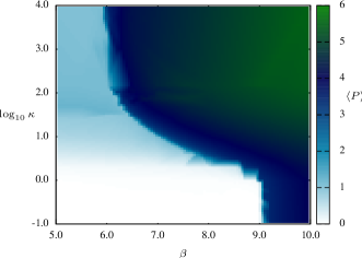
Figure 3: Expectation values of $P$ in the coupling constant plane and on a small $12^{3}\times 2$ lattice

We see that in the confining phase the expectation value varies from $0$ to $1$ when the hopping parameter increases. For large values of $\beta$ in the unconfined phase the Polyakov loop is near the identity or (for large $\kappa$) near one of the three center-elements of $SU(3)$. On the small lattice the Polyakov loop jumps along a continuous curve connecting the confinement-deconfinement transitions of pure $G_{2}$ and pure $SU(3)$ gluodynamics. This suggests that there exists a connected first order transition curve all the way from $\kappa=0$ to $\kappa=\infty$. To see whether this is indeed the case we performed high-precision simulations on larger lattices. A careful analysis of histograms and susceptibilities for Polyakov loops and the Higgs action shows that the first order lines beginning at $\kappa=0$ and at $\kappa=\infty$ do not meet. This happens in a rather small region in parameter space such that the two first order lines almost meet. They may be connected by a line of continuous transitions or in-between there may exists a window connecting the confined and unconfined phases smoothly.

For $\beta\to\infty$ we are left with a nonlinear $O(7)$ sigma model with action

$$S_{\sigma}=-\kappa\sum\limits_{x,\mu}\Phi_{x+\hat{\mu}}\Phi_{x}\,,$$ (27)

and this model shows a second order transition at a critical coupling $\kappa_{c}$ from a $O(7)$ symmetric to a $O(6)$ symmetric phase. To see how this transition continues to finite values of $\beta$ we measured the expectation values $\langle\mathcal{O}_{P}\rangle$ and $\langle\mathcal{O}_{H}\rangle$ of the (averaged) plaquette variable and Higgs action

$$\mathcal{O}_{P}=\frac{1}{7\cdot 6\cdot V}\sum_{\square}\operatorname{Re}\operatorname{tr}\mathcal{U}_{\square}\quad\hbox{and}\quad\mathcal{O}_{H}=\frac{1}{V}\sum\limits_{x\mu}\Phi_{x+\hat{\mu}}\,\mathcal{U}_{x,\mu}\Phi_{x}\,.$$ (28)

and the corresponding susceptibilities

$$\chi(\mathcal{O})=V\left(\langle\mathcal{O}^{2}\rangle-\langle\mathcal{O}\rangle^{2}\right)\,.$$ (29)

The finite size scaling theory predicts that near the transition point the maximum of the susceptibilities scales with the volume to the power of the corresponding critical exponent $\gamma$

$$\chi(\mathcal{O})\sim aL^{\gamma/\nu}+b\,,$$ (30)

where $\nu$ is the critical exponent related to the divergence of the correlation length. For a first order phase transition we expect the susceptibility peak to scale linearly with the spatial volume (since $N_{t}$ is fixed). More precisely, for a first order transition one expects $\gamma=1$ and $\nu=1/3$ while for a second order transition $\gamma\neq 1$ Binder:1984 .

The expectation values and logarithms of susceptibilities on a small $6^{3}\times 2$-lattice are depicted in Fig. 4.

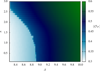
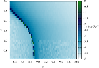
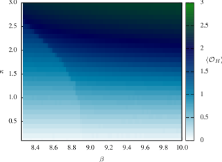
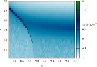
Figure 4: Average plaquette, Higgs action and susceptibilities near the critical point on $6^{3}\times 2$ lattice.

The expectation value of a plaquette variable jumps at the deconfinement transition line and the corresponding susceptibility is peaked. This is in full agreement with the jump of the Polyakov loop across this transition line. The expectation value of the Higgs action and the corresponding susceptibility both spot the deconfinement transition well. But they also discriminate between the $O(7)$ unbroken and broken phases. The data on the small lattice point to a second order Higgs transition line in the YMH-model for all $\beta>\beta_{\rm deconf}(\kappa)$. This could imply that the second order line ends at the first order deconfinement transition line. To determine the order of the Higgs transition line we consider the finite size scaling of

$$\chi(\mathcal{O}_{H})=\frac{\partial}{\partial\kappa}\left\langle\mathcal{O}_{H}\right\rangle\quad\hbox{and}\quad\frac{\partial^{2}}{\partial^{2}\kappa}\left\langle\mathcal{O}_{H}\right\rangle$$ (31)

for lattices up to $20^{3}\times 6$. The results presented below show that the Higgs transitions are second order transitions. Unfortunately we cannot exclude the possibility that the second order line turns into a crossover near the deconfinement transition line.

Our results on the complete phase diagram in the $(\beta,\kappa)$-plane as calculated on a larger $16^{3}\times 6$-lattice are summarized in Fig. 5. We calculated histograms and susceptibilities near the marked points on the transition lines in this figure. If the triple point exists then an extrapolation to the point where the confined phase meets both unconfined phases leads to the couplings $\beta_{\text{trip}}=9.62(1)$ and $\kappa_{\text{trip}}=1.455(5)$.

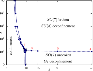
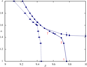
Figure 5: Phase transition lines on a $16^{3}\times 6$ lattice. The solid line corresponds to the first order deconfinement transitions, the dashed line to the second order Higgs transitions and the dotted line to the left of the first order line to the bulk transitions. The plot on the right shows the details inside the small box in the plot on the left where the transition lines almot meet.

Near this point the deconfinement transition is very weak, continuous or absent and thus we performed high-statistics simulations on larger lattices to investigate this region in parameter space more carefully. Some of our results are presented in the following sections. Up to a rather small region surrounding $(\beta_{\text{trip}},\kappa_{\text{trip}})$ we can show that the deconfinement transition is first order and the Higgs transition is second order. But we shall see that in a small region around this point the deconfinement transition is either second order or absent.

The bulk transition

The existence of a bulk transition in lattice gauge theories at zero temperature can influence its finite temperature behaviour. Such transitions are almost independent of the size of the lattice and are driven by lattice artifacts Halliday:1981te . Bulk transitions between the unphysical strong-coupling and the physical weak-coupling regimes in lattice gauge theories is the rule rather than the exception. The strong coupling bulk phase contains vortices and monopoles which disorder Wilson loops down to the ultraviolet length scale given by $a^{2}\sigma\sim O(1)$ Lucini:2005vg ; Brower:1981 . In the weak coupling phase the short distance physics is determined by aymptotic freedom and $a^{2}\sigma\ll 1$. Both $SU(2)$ and $SU(3)$ lattice theories exhibit a rapid crossover between the two phases which beomes more pronounced for $SU(4)$ Lucini:2005vg . For $SU(N)$ with $N\geq 5$ the bulk transition is first order Lucini:2005vg . $SU(3)$ lattice gauge theory with mixed fundamental ($f$) and adjoint ($a$) actions shows a first order bulk transiton for large $\beta_{a}$ and small $\beta_{f}$. For decreasing $\beta_{a}$ the transition line terminates at a critical point and turns into a crossover touching the line $\beta_{a}=0$. On lattices with $N_{t}=2$ the deconfinement transition line joins the bulk transition line smoothly from below and for $N_{t}\geq 4$ from above Caneschi:1981ik ; Blum:1994xb . More relevant for us is the finding in Cossu:2008 that the bulk transition in pure $G_{2}$ gauge theory at $\beta=9.45$ is a crossover Cossu:2008 .

We have scanned the values for the plaquette variables and Polyakov loops from the strong to the weak coupling regime to find a bulk transition that might interfere with the finite temperature deconfinement transition. For various values between $\kappa=0$ and $\kappa=\infty$ on a $12^{3}\times 6$ and $16^{3}\times 6$ lattice we determined the position and nature of the bulk transitions. In full agreement with Cossu:2008 we see a crossover at $(\beta,\kappa)\approx(9.44,0)$ which is visible as a broad peak in the plaquette susceptibility depicted in the right panel of Fig. 6. The Polyakov loop does not detect this crossover.

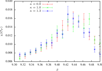
Figure 6: Plaquette and susceptibility for small values of $\kappa$ near the bulk transition on a $12^{3}\times 6$ lattice.

Note that for small $\kappa$ the position of the bulk transition does not depend on the hopping parameter which means that the bulk transition line hits the line $\kappa=0$ vertically. Despite of the broad peak in the susceptibility of the plaquette density are the bulk and deconfinement transition cleary separated and this agrees with the results in Bonati:2009pf . In the region $1.3\leq\kappa\leq 1.6$ the critical coupling $\beta_{c}$ decreases with increasing $\kappa_{c}$ but the nature of the transition does not change much as can bee seen in Fig. 7.

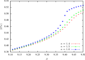
Figure 7: Plaquette and susceptibility for intermediate values of $\kappa$ near the bulk transition on a $12^{3}\times 6$ lattice.

The plaquette density seems to be a continous function of $\beta$ and $\kappa$ and we conclude that the transition is still a crossover.

Between $\kappa=1.6$ and $\kappa=1.65$ the peak in the bulk transition becomes pronounced. In this region the distance between the bulk and deconfinement transitions becomes very small. Nevertheless we expect that the much localized bulk transition still does not interfere with the weak deconfinement transition. For values of $\kappa$ between $1.65$ and approximately $2.5$ the position of the bulk transition gets more sensitive to the hopping parameter and the distance to the deconfinement transition line increases again. The nature of the transition changes at the same time – a large gap in the action density separates the strong coupling from the weak coupling region. This is depicted in Fig. 8.

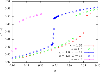
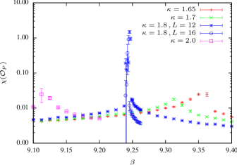
Figure 8: Plaquette and susceptibility for intermediate values of $\kappa$ near the bulk transition on $12^{3}\times 6$ lattice.

The many data points taken at $\kappa=1.8$ show that the size of the gap does not depend on the volume and this points to a first order transition. The plots for the plaquettes and plaquette susceptibilites look very much like the plots in Fig. 6. For $\kappa\gtrsim 2.5$ the situation changes again. The gap in the plaquette density closes and the position of the bulk transition tends to that of the bulk transition in $SU(3)$ gluodynamics which again is a crossover.

There is ample evidence that bulk transitions are driven by monopoles on the lattice Halliday:1981te . Thus we calculated the density of monopoles Caneschi:1981ik as a function of $\beta$ for $\kappa=0$ and $\kappa=1.8$. The density $M$ together with the plaquette variable are plotted in Fig. 9.

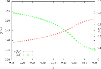
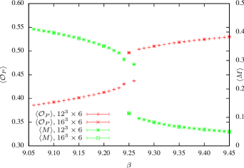
Figure 9: Plaquette and Monopole density for $\kappa=0$ and $\kappa=1.8$ on a $12^{3}\times 6$ and $16^{3}\times 6$ lattice.

For $\kappa=0$ they vary smoothly with $\beta$, as expected for a cross-over, but for $\kappa=1.8$ they jump at the same $\beta\approx 9.25$. The height of the jump does not depend on the lattice size, see Fig. 9, right panel. Thus we find strong evidence that the bulk transition is intimately related to the condensation of monopoles in the strong coupling $G_{2}$ Higgs model.

Finally we would like to comment on the behaviour near $\kappa=1.6$. Here the $G_{2}$ Higgs model behaves similar to $SU(3)$ gluodynamics with mixed fundamental and adjoint actions. The latter shows a first order bulk transition which turns into a crossover for small $\beta_{a}$. It seems that for $\kappa\gtrsim 1.6$ the massive $G_{2}$-gluons are heavy enough such that the approximate center symmetry of the unbroken $SU(3)$ is at work. This could explain why we find a first order transition for $\kappa\gtrsim 1.6$.

V The transition lines away from the triple point

In this section we come back to the confinement-deconfinement transition. Sufficiently far away from the suspected triple point at $\beta_{\text{trip}}=9.62(1)$ and $\kappa_{\text{trip}}=1.455(5)$ the signals for first- and second order phase transitions are unambiguous and are presented in this section. The measurements taken near the would-be triple point are less conclusive and will be presented and analysed in the following section.

The confinement-deconfinement transition line

Already the histograms for the Polyakov loop show that the deconfinement transition is first order for values of the hopping parameter $\kappa$ in the intervals $[0,1.4]$ and $[1.7,\infty]$.

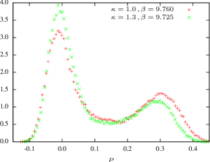
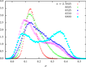
Figure 10: Distributions of the Polyakov loop on a $16^{3}\times 6$-lattice. Left panel: $(\beta,\kappa)=(9.76,1)$ and $(9.725,1.3)$; Right panel: $\beta=9$ and various values of the hopping parameter.

Two typical distributions for $\kappa=1.0$ and $\kappa=1.3$ corresponding to the points $1$ and $2$ in the phase diagram in Fig. 5 are depicted in Fig. 10 (left panel). These and other histograms with $\kappa\lesssim 1.4$ show a clear double peak structure near the transition line and are almost identical to the histogram for $\kappa=0$. Similar results are obtained for larger hopping parameters $\kappa\gtrsim 1.7$.

In Fig. 10 (Right panel) we plotted histograms of the Polyakov loops for $\beta=9$ and hopping parameters in the vicinity of $\kappa\approx 2.6$, corresponding to point $3$ in Fig. 5. The histograms with $\kappa\leq 2.6525$ show peaks at almost the same positions. The systems with these small values of $\kappa$ are in the confined phase. For larger $\kappa$-values the peak moves towards the ’would-be’ center elements of the subgroup $SU(3)$ and a second peak appears. Again the double-peak structure of the distribution points to a first order transition. We varied the spatial sizes of the lattices and observed no finite size effects in the distributions for $N_{s}\geq 16$.

The Higgs transition line

For $\beta\to\infty$ the gauge degrees of freedom are frozen and we are left with a nonlinear $O(7)$ sigma-model which shows a second order transition from a $O(7)$-symmetric massive phase to a $O(6)$-symmetric massless phase. With the help of a cluster algorithm Wolff:1989 we updated the constrained scalar fields and calculated the susceptibility of

$$\mathcal{O}_{\sigma}=\frac{1}{V}\sum_{x,\mu}\Phi_{x+\hat{\mu}}\Phi_{x}$$ (32)

which is proportional to the sigma-model action $S_{\sigma}$ in (27),

$$\chi(\mathcal{O}_{\sigma})=-\frac{1}{\kappa V}\,\partial_{\kappa}\langle S_{\sigma}\rangle.$$ (33)

The results of our simulations on lattices with varying spatial sizes are depicted in Fig. 11, left panel.

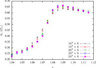
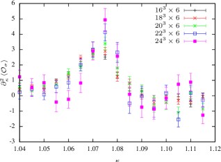
Figure 11: The first and second derivative of the average sigma-model action for different spatial lattice sizes.

The susceptibility of the action becomes steeper as the spatial volume increases while the peak of the (normalized) second derivative also increases. This means that the system undergoes a second order transition at $\kappa_{c}=1.075(5)$ (corresponding to point $4$ in Fig. 5) from a massive $O(7)$-symmetric phase with vanishing vacuum expectation value to a massless $O(6)$-symmetric phase with non-vanishing expectation value. Actually the mean field theory for $O(n)$ models in $d$ dimensions predicts a second order transition at the critical coupling $\kappa_{c,\rm mf}=n/2d$. For our model in $4$ dimensions the mean-field prediction is $\kappa_{c,\rm mf}=7/8\approx 0.875$ and is not far from our numerical value.

For smaller values of $\beta$ the gauge degrees of freedom participate in the dynamics and $\partial_{\kappa}\langle S\rangle$ is now proportional to the susceptibility of $\mathcal{O}_{H}$ in (28). The plots in Figs. 12 and 13 show a similar behavior of the first and second derivatives of the average Higgs action for $\beta=30$ and $12$, corresponding to the points $5$ and $6$ in the phase diagram in Fig. 5.

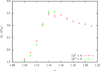
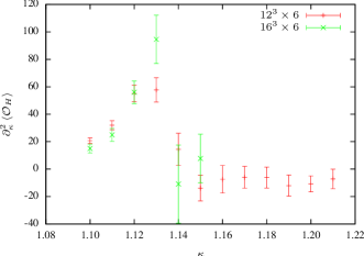
Figure 12: First and second derivative of the average action with respect to the hopping parameter for different spatial lattice sizes at $\beta=30$

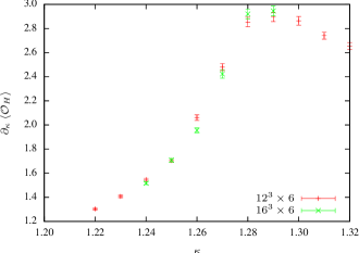
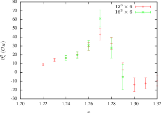
Figure 13: First and second derivative of the average action with respect to the hopping parameter for different spatial lattice sizes at $\beta=12$

Even for the smaller value $\beta=12$ we see that the susceptibility becomes steeper with increasing lattice size while the second derivative of the average action increases. This already demonstrates that the second order transition at the aymptotic region $\beta\to\infty$ extends to smaller values of $\beta$.

VI The transition lines near the triple point

When the first order transition become weaker it becomes increasingly difficult to distinguish it from a second order transition or a cross-over. For example, the four histograms in Fig. 14 show distributions of the Polyakov loop at point $7$ in the phase diagram depicted in Fig. 5, corresponding to $\kappa=1.5$ and $\beta$ varying between $9.5525$ and $9.5550$. All histograms are computed from $400\,000$ configurations on a medium size $16^{3}\times 6$ lattice. The histogram on top left shows a pronounced peak at $P\approx 0.1$, corresponding to the value in the confined phase. With increasing $\beta$ a second peak builds up at $P\approx 0.25$ corresponding to a value in the unconfined phase. We have calculated more histograms and conclude that the well-separated peaks in the distribution are of equal heights for $\beta_{c}\approx 9.5535$. At this point the Polyakov loop jumps from the smaller to the larger value. For even larger values of $\beta$ the second peak at larger $P$ takes over and the system is in the unconfined phase.

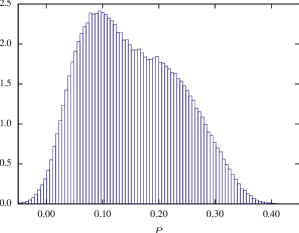
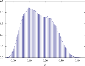
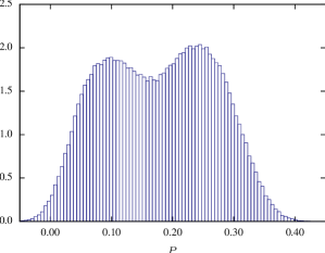
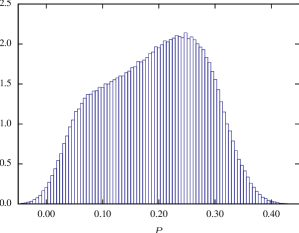
Figure 14: Distributions of the Polyakov loop at $\kappa=1.5$ where the transition is weakly first order on a $16^{3}\times 6$ lattice with $400\,000$ configurations for each histogram. Top left $\beta=9.5525$, top right $\beta=9.5535$, bottom left $\beta=9.5540$ and bottom right $\beta=9.5550$ ($\beta_{c}\approx 9.5535$).

Although the histograms point to a weakly first order transition we can not rule out the possibility that the transition at $\kappa=1.5$ and $\beta\approx 9.5535$ is of second order. Later we shall see that it is a first order transition. If we slightly decrease the value of $\kappa$, then the signal for a first order transition is more pronounced. This is illustrated in the Polyakov loop histograms depicted in Fig. 15. If we again increase the value from $\kappa=1.5$ to $\kappa=1.55$ the peak of the Polyakov loop does not jump at the transition point at $\beta\approx 9.4885$. Instead it increases smoothly from $P\approx 0.12$ in the confinement phase to $P\approx 0.24$ in the deconfinement phase, see Fig. 16. We conjecture that in this region of parameter space the first order transition turns into a continuous transition or a cross-over which is later confirmed by an even more careful analysis.

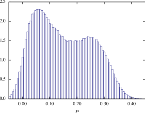
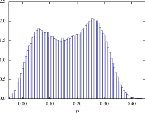
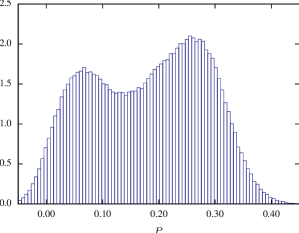
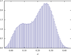
Figure 15: Distribution of the Polyakov loop at $(\beta,\kappa)=(9.6190,1.455)-(9.6220,1.455)$ near the supposed triple point; $400\,000$ configurations on $16^{3}\times 6$ lattice

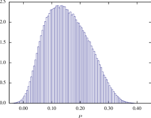
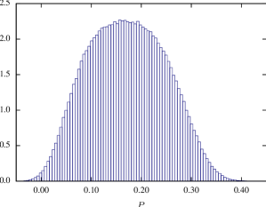
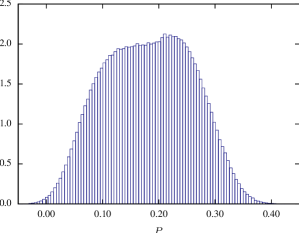
Figure 16: Distributions of the Polyakov loop at $\kappa=1.55$ where the transition is probably not first order on a $16^{3}\times 6$ lattice with $800\,000$ configurations for each histogram. Top left $\beta=9.4875$, top right $\beta=9.4885$, bottom left $\beta=9.4895$ and bottom right $\beta=9.4905$ ($\beta_{c}\approx 9.4885$).

We studied the size-dependence of the average Polyakov loop, plaquette variable and Higgs-action per lattice site together with their susceptibilities. The following results are obtained on lattices with $N_{t}=6$ and spatial extends $N_{s}\in\{12,16,20,24\}$ and for $\beta=9.5535$. This corresponds to points in the neighborhood of point $7$ in the phase diagram in Fig. 5.

Fig. 17 shows the $\kappa$-dependence of the Polyakov loop and its susceptibility for the four different lattices. The measurements have been taken at $20$ different values of the hopping parameter in the vicinity of $\kappa=1.5$.

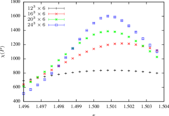
Figure 17: Finite size scaling of Polyakov loop and Polyakov loop susceptibility at $\beta=9.5535$

This way we cross the phase transition line vertically in the $\kappa$-direction at the transition point $7$ in the phase diagram in Fig. 5. The $\kappa$-dependence has been calculated with the reweighting method. Later we shall see that the peak of the susceptibility at $\kappa_{c}\approx 1.501$ scales linearly with the volume. This linear dependence is characteristic for a first order transition.

The plots in Fig. 18 show the $\kappa$-dependence of the average plaquette variable and the corresponding susceptibility for the four lattices. Again we observe that the susceptibility peak at $\kappa_{c}\approx 1.501$ increases linearly with the volume of the lattice. Also note that on the small $12^{3}\times 6$ lattice the peak in the susceptibility can hardly be seen.

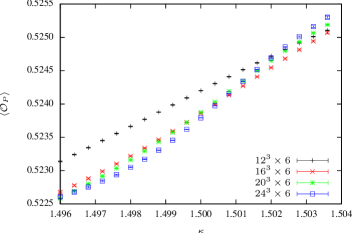
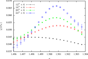
Figure 18: Finite size scaling of the plaquette variable and its susceptibility for $\beta=9.5535$.

The two plots in Fig. 19 show the $\kappa$-dependence of the average Higgs action per lattice point and corresponding susceptibility. Similarly as for the Polyakov loop and the plaquette we observe a peak of the susceptibility at the same value $\kappa_{c}\approx 1.501$.

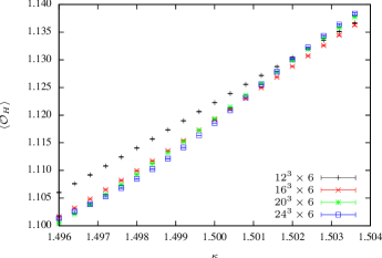
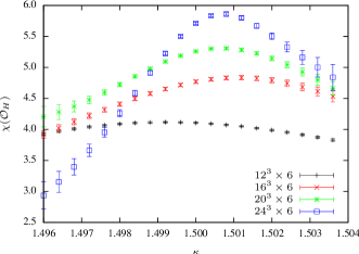
Figure 19: Finite size scaling of Higgs action and its susceptibility for $\beta=9.5535$.

To check for finite size scaling we investigated the susceptibilities corresponding to the Polyakov loop, plaquette variable and Higgs-action per site as a function of the volume. The results are plotted in Fig. 20, left panel. For an easier comparison we normalized the data points by the peak value for the largest lattice with lattice size $N_{s}=24$. The linear dependence of the peak susceptibilities on the volume is clearly visible for the larger three lattices and this linear dependence is predicted by a first order transition Binder:1984 . In recent studies of the lattice $SU(2)$ Higgs model in Bonati:2009pf it turned out that for $N_{s}=N_{t}\lesssim 18$ the maxima of the susceptibilities are well described by a function of the form $aL^{4}+b$, so that they seem to scale linearly with volume, as expected for a first order transition at zero temperature. Simulations on larger lattices revealed however, that the suceptibility peaks all saturate at larger values of $L$ and no singularities seems to develop in the thermodynamic limit. For the lattice $G_{2}$-Higgs model considered in the present work we see no flattening of the peaks for larger lattices with $N_{s}$ up to $24$ and we interpret this as a signal for a true first order transition.

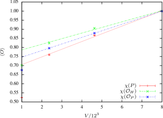
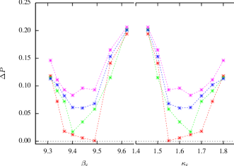
Figure 20: Left panel: finite size scaling of the three susceptibilities at the transition point with $\beta=9.5535.$ The lines are fits to the peak values, $\chi_{\rm max}(V)=aV+b$. Right panel: Difference of Polyakov loop in confined and unconfined phase at the phase transition point for various couplings $\beta,\kappa$ and various intervalls around the critical coupling coupling $\beta_{c}$, red: $\Delta\beta=0.0005$, green: $\Delta\beta=0.0015$, blue: $\Delta\beta=0.0025$, pink: $\Delta\beta=0.0035$, $\kappa$ is fixed ($\Delta\kappa=0$)

Table 3 shows the extrapolation of the critical hopping parameter to infinite volumes. To that end we calculated for each lattice size the value $\kappa_{c}(V)$ at which the Polyakov loop-, plaquette- and Higgs action susceptibilities take their maxima. Note that on the larger lattices with $N_{s}=20$ and $24$ the three critical hopping parameters are the same within statistical errors. The infinite volume extrapolation yields the critical value $\kappa_{c}=1.5008$.

Volume	$12^{3}$	$16^{3}$	$20^{3}$	$24^{3}$
$\chi(P)$	$1.5012$	$1.5016$	$1.5008$	$1.5008$
$\chi(\mathcal{O}_{H})$	$1.4992$	$1.5012$	$1.5008$	$1.5008$
$\chi(\mathcal{O}_{P})$	$1.4980$	$1.5008$	$1.5008$	$1.5008$

Table 3: Critical coupling $\kappa_{c}$ obtained from the maximum of the susceptibility peaks of Polyakov loop, plaquette and Higgs action for different spatial volumes at $\beta=9.5535$

VI.1 The first order lines do not meet

The previous results on the $16^{3}\times 6$ lattice leave a small region in parameter space near $(\beta,\kappa)\approx(9.4,1.6)$, where the transition may be continuous or where we can cross smoothly between the confined and unconfined phases. Since a jump of the Polyakov loop expectation values in the infinite volume limit points to a first order transition we investigated the quantity

$$\Delta P=\langle P\rangle_{\rm deconfined}-\langle P\rangle_{\rm confined}$$ (34)

more carefully. In the small parameter region we localized the critical curve $(\beta_{c},\kappa_{c})$ with the histogram method. At the critical point is the height of the confinement peak equal to the height of the deconfinement peak. For fixed $\kappa_{c}$ we crossed the transition line by increasing the inverse gauge coupling. Then we measured the maximal jump as a function of the step size $\Delta\beta$ for one step size below and one above $\beta_{c}$. For a first order transition the jump should not depend much on $\Delta\beta$ whereas for a continuous transition or a cross-over $\Delta P$ should decrease with decreasing $\Delta\beta$. The results on a $16^{3}\times 6$ lattic are depicted in Fig. 20 (right panel). We see that for $9.35\lesssim\beta_{c}\lesssim 9.52$ corresponding to $1.52\lesssim\kappa_{c}\lesssim 1.72$ the jump approaches zero with shrinking step size and this clearly points to second order confinement-deconfinement transitions or cross-overs in these small parameter regions. Simulations on a larger $20^{3}\times 6$ lattice confirm these results. Fig. 21 shows histograms of the Polyakov loop for $\kappa$-values between $1.5$ and $1.7$. At $\kappa=1.5$ we still observe a weakly first order transition which turns into a continuous transition or crossover for $1.5<\kappa\leq 1.7$. Within the given resolution in parameter space the window is the same as on the $16^{3}\times 6$ lattice. Since the critical couplings for spatial volumes beyond $20^{3}$ do not change we conclude that the gap will not close in the infinite volume limit. This shows that the two first order lines emanating from $\kappa=0$ and $\kappa=\infty$ do not meet.

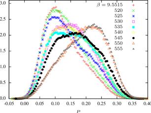
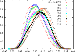
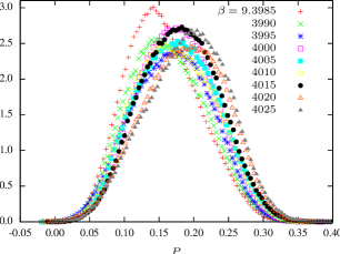
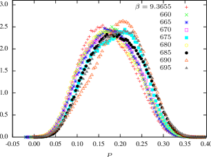
Figure 21: Distribution of Polyakov loop near the phase transition point for $\kappa=1.5$ (top left), $\kappa=1.55$ (top right), $\kappa=1.65$ (bottom left) and $\kappa=1.7$ (bottom right) on a $20^{3}\times 6$ lattice

Here the question arises whether such a gap in the first order line between the confined and unconfined phases is expected. The celebrated Fradkin-Shenker-Osterwalder-Seiler theorem Osterwalder:1977pc ; Fradkin1979 , originally proven for the $SU(N)$ Higgs-model with scalars in the fundamental representation, says that there is no complete separation between the Higgs- and the confinement regions. Any point deep in the confinement regime and any point deep in the Higgs regime are related by a path such that Green’s functions of local, gauge invariant operators vary analytically along the path. Thus there is no abrupt change from a colorless to a color-charged spectrum. This is consistent with the fact that there are only color singlet asymptotic states in both ’phases’.

The proof of the theorem relies crucially on using a completely-fixed unitary gauge. A complete gauge fixing is not possible with scalars in the adjoint representation of $SU(N)$ since these scalars are center blind. Thus the theorem does not hold for adjoint scalars and indeed, with adjoint scalars there exits a phase boundary separating the Higgs and confined phases. It is not completely obvious what these results tell us about the phase diagram of the $G_{2}$ Higgs model. The center of $G_{2}$ is trivial and the $14$-dimensional adjoint representation is just one of the two fundamental representations. Since there is no need to break the center one may conclude that the confinement-like regime and the Higgs-like regimes are analytically connected. In addition, for large values of the hopping parameter the center of the corresponding $SU(3)$ gauge theory is explicitly broken by the scalar fields, simililarly as for the $SU(3)$ Higgs model with scalars in the fundamental representation. These arguments suggest that there exist a smooth cross-over between the confining and Higgs phases. But one important assumption of the Fradkin-Shenker theorem is not fulfilled for the $G_{2}$ Higgs model. The theorem assumes that there exists no transition for large $\kappa$. Then at large $\kappa$ one can move from large to small $\beta$ and then at small $\beta$ further on to small values of $\kappa$ without hitting a phase transition. Clearly this is not possible for the $G_{2}$ Higgs model such that not all assumption of the theorem hold true.

VII Conclusions

With a new and fast LHMC-implementation for the exceptional $G_{2}$ Higgs model we calculated the full phase diagram in the coupling constant plane spanned by the hopping parameter $\kappa$ and inverse gauge coupling $\beta$. First we confirmed the proposed and earlier seen Pepe:2006er ; Cossu:2008 first order transition for pure $G_{2}$-gluodynamics which corresponds to the line $\kappa=0$ in the phase diagram of the Higgs model. A first analysis on smaller lattices indicated that this first order transition is connected to the first order deconfinement transition in $SU(3)$-gluodynamics, corresponding to the limit $\kappa\to\infty$, by a smooth curve of first order transitions. The same analysis spotted another curve of second-order transitions emanating from $\beta\to\infty$ and meeting the first order line at a triple point. For this first analysis we calculated histograms for the Polyakov loop, Higgs-action and plaquette action. To identify the second order transition line we studied the finite size scaling of various susceptibilities and the second derivative of the action with respect to the hopping parameter. The final result of our analysis on a $16^{3}\times 6$ lattice is depicted in Fig. 22. Note that the tiny region in the vicinity of the would-be triple point is very much enlarged in this figure.

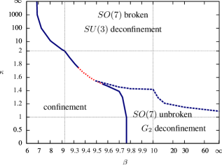
Figure 22: Complete phase diagram in the $(\beta,\kappa)$-plane on a $16^{3}\times 6$ lattice. The neighbourhood of the ’would-be triple point’ is very much enlarged and the variable scale in the diagram is responsible for the cusps in the transition lines. The solid line indicates a first order transition, the dashed line (blue) a second order transition and the dotted line (red) a second oder transition or a crossover.

In this tiny region in the $(\beta,\kappa)$-plane where the order of the transition could not be decided we studied the slope of $\langle P\rangle$ in the vicinity of the suspected transition. The simulations show that the two first-order curves emanating from the lines with $\kappa=0$ and $\kappa=\infty$ end before they meet. The two curves could be connected by a line of second-order transition or they could end at two (critical) endpoints in which case the confined and unconfined phases are smoothly connected. If indeed there exists a cross-over in $G_{2}$ Higgs model at a finite value of the hopping parameter then the gauge model behaves very similar to QCD with massive quarks.

To finally answer the question about the behavior of $G_{2}$ Higgs model theory in the vicinity of the ’would-be triple point’ at $(\beta,\kappa)\approx(9.4,1.6)$ further simulations with an even higher statistics and a more sophisticated analysis of the action susceptibilities may be necessary. Since we already used an efficient (and parallelized) LHMC-algorithm and much CPU-time to arrive at the results presented in the work this will not be an easy task. Earlier studies of the susceptibility peaks in the simpler $SU(2)$-Higgs model on smaller lattices pointed to a first order transition at $\beta\lesssim 2.5$. Recent simulations on larger lattices in Bonati:2009pf showed that the susceptibility peaks do not scale with the volume such that there is actually no first order transition for these small values of $\beta$. We have seen no flattening of the peaks with the increasing volumes for $N_{s}\leq 24$ and conclude that the solid line in Fig. 22 is a first order line. But of course we cannot exclude the possibility that the correlation length is larger as expected and that simulations on even larger lattices are necessary to finally settle the question about the position and size of the window connecting the confined with the unconfined phase. This will not be easy and thus it would be very helpful to actually prove that the confining and Higgs phases of $G_{2}$ can be connected analytically, perhaps with similar arguments as they apply to $SU(N)$ Higgs models with matter in the fundamental representations Osterwalder:1977pc ; Fradkin1979 .

- (1) B. Svetitsky and L. G. Yaffe, Critical Behavior at Finite Temperature Confinement Transitions, Nucl. Phys. B210 (1982) 423.
- (2) L. G. Yaffe and B. Svetitsky, First Order Phase Transition in the SU(3) Gauge Theory at Finite Temperature, Phys. Rev. D26 (1982) 963.
- (3) C. Wozar, T. Kästner, A. Wipf, T. Heinzl and B. Pozsgay, Phase Structure of Z(3)-Polyakov-Loop Models, Phys. Rev. D74 (2006) 114501 [arXiv:hep-lat/0605012].
- (4) A. Wipf, T. Kaestner, C. Wozar, T. Heinzl, Generalized Potts-Models and their Relevance for Gauge Theories, Sigma 3 (2007) 006
- (5) J. Greensite, The confinement problem in lattice gauge theory, Prog. Part. Nucl. Phys. 51 (2003) 1.
- (6) M. Pepe and U. J. Wiese, Exceptional Deconfinement in G(2) Gauge Theory, Nucl. Phys. B768 (2007) 21 [arXiv:hep-lat/0610076].
- (7) K. Holland, M. Pepe and U. J. Wiese, The unconfined phase transition of Sp(2) and Sp(3) Yang-Mills theories in 2+1 and 3+1 dimensions, Nucl. Phys. B694 (2004) 35 [arXiv:hep-lat/0312022].
- (8) K. Holland, P. Minkowski, M. Pepe and U. J. Wiese, Exceptional confinement in G(2) gauge theory, Nucl. Phys. B668 (2003) 207 [arXiv:hep-lat/0302023].
- (9) J. Greensite, K. Langfeld, S. Olejnik, H. Reinhardt and T. Tok, Color screening, Casimir scaling, and domain structure in G(2) and SU(N) gauge theories, Phys. Rev. D75 (2007) 034501 [arXiv:hep-lat/0609050].
- (10) J. Danzer, C. Gattringer, A. Maas, Chiral symmetry and spectral properties of the Dirac operator in G2 Yang-Mills Theory, JHEP 0901 (2009) 024. [arXiv:hep-lat/:0810.3973]
- (11) A. Maas, S. Olejnik, A First look at Landau-gauge propagators in G(2) Yang-Mills theory, JHEP 0802 (2008) 070. [arXiv:hep-lat/0711.1451]
- (12) L. Liptak and S. Olejnik, Casimir scaling in G(2) lattice gauge theory, Phys. Rev. D78 (2008) 074501 [arXiv:0807.1390].
- (13) B. Wellegehausen, A. Wipf and C. Wozar, Casimir Scaling and String Breaking in G(2) Gluodynamics, Phys. Rev. D83 (2011) 016001 [arXiv:hep-lat/1006.2305]
- (14) B. Wellegehausen, A. Wipf, C. Wozar, Effective Polyakov Loop Dynamics for Finite Temperature G(2) Gluodynamics. Phys. Rev. D80 (2009) 065028.
- (15) B. Simon, Mean field upper bound on the transition temperature in multicomponent ferromagnets, J. Stat. Phys. 20 (1980) 491.
- (16) G. Cossu, M. D’Elia, A. Di Giacamo, B. Lucini, C. Pica, gauge theory at finite temperature, JHEP 10 (2007) 100 [arXiv:hep-th/0709.0669]
- (17) A. J. Macfarlane, The sphere S(6) viewed as a G(2)/SU(3) coset space, Int. J. Mod. Phys. A17 (2002) 2595.
- (18) P. Marenzoni, L. Pugnetti and P. Rossi, Measure Of Autocorrelation Times Of Local Hybrid Monte Carlo Algorithm For Lattice QCD, Phys. Lett. B 315 (1993) 152.
- (19) K. Binder, D.P. Landau Finite-size scaling at first order phase transitions, Phys. Rev. B30 (1984) 1477.
- (20) I.G. Halliday, A. Schwimmer, The phase structure of SU(N)/Z(N) lattice gauge theories, Phys.Lett. B101 (1981) 327.
- (21) B. Lucini, M. Teper, Michael, U. Wenger, Properties of the deconfining phase transition in SU(N) gauge theories, JHEP 02 (2005) 33 [arXiv:hep-lat/0502003]
- (22) C. R. Brower, D. A. Kessler, H. Levine Monopole Condensation and the Lattice-Quantum-Chromodynamics Crossover, Phys. Rev. Lett. 47 (1981) 621.
- (23) T. Blum, C. DeTar, U. Heller, L. Kärkkäinen, K. Rummukainen, D. Toussaint Thermal phase transition in mixed action SU(3) lattice gauge theory and Wilson fermion thermodynamics, Nucl. Phys. B442 (1995) 301 [arXiv:hep-lat/9412038].
- (24) L. Caneschi, I. G. Halliday, A. Schwimmer THE PHASE STRUCTURE OF MIXED LATTICE GAUGE THEORIES, Nucl. Phys. B200 (1982) 409.
- (25) C. Bonati, G. Cossu, M. D’Elia, A. Di Giacomo, Phase diagram of the lattice SU(2) Higgs model, Nucl. Phys. B828 (2010) 390.
- (26) U. Wolff, Collective Monte Carlo Updating for Spin Systems, Phys. Rev. Lett. 62 (1989) 361.
- (27) K. Osterwalder, E. Seiler, Gauge Field Theories on a Lattice, Ann. Phys. 110 (1978) 440.
- (28) E. Fradkin, S.H. Shenker, Phase diagram of Lattice gauge theories with Higgs fields, Phys. Rev. D19 (1979) 3682.
- (29) M. Grady, Reconsidering gauge-Higgs continuity, Phys. Lett. B626 (2005) 161.