Generalized thermodynamic uncertainty relations

Abstract: We analyze an ensemble in which energy ($E$), temperature ($T$) and multiplicity ($N$) can all fluctuate and with the help of nonextensive statistics we propose a relation connecting all fluctuating variables. It generalizes Lindhard’s thermodynamic uncertainty relations known in literature.

PACS: 05.20.-y 05.70.-a 12.40.Ee

Keywords: Thermodynamics, Nonextensive statistics, Fluctuations

1 Introduction

A long time ago, it was suggested that the thermodynamical quantities, temperature $T$ and energy $U$, could be regarded as being complementary in the same way as are position and momentum in quantum mechanics [1]. The reason is that the only way to attribute a definite temperature to a physical system is by bringing it into thermal contact and equilibrium with another very large system acting as a heat bath. In this case, however, the system will freely exchange energy with the heat bath, and one loses the possibility of controlling its energy. On the other hand, in order to make sure that the system has a definite energy, one should isolate it from its environment. But then there is no way to determine its temperature. Dimensional analysis already leads to the conjecture that this relation would take the form $\Delta U\,\Delta\beta\geq k$, where $\beta=1/T$ and $k$ is Boltzmann’s constant. The isolation ($U$ definite) and contact with a heat bath ($T$ definite) then represent two extremal cases of such complementarity. This idea has so far not received much recognition in the literature because its validity and foundations are under discussion (see [2] for review and [3] for comments). The main point is the exact meaning of the increments $\Delta$. Indeed, all versions of this uncertainty relation proposed so far employ different theoretical frameworks and give different interpretations of the uncertainty $\Delta\beta$, in most cases by using concepts from theories of statistical inference.

In this paper we shall treat these increments as a measure of fluctuation of the corresponding physical quantities and analyze an ensemble in which energy ($U$), temperature ($T$) and multiplicity ($N$), can all fluctuate. In this way we generalize the relation between fluctuations of $U$ and $T$ derived in thermodynamics [4] expressed by their relative variances $Var(x)/\langle x\rangle^{2}=\omega^{2}_{x}$ as:

$$\omega_{U}^{2}\,+\,\omega^{2}_{T}\,=\,\frac{1}{\langle N\rangle}.$$ (1)

Eq. (1) is an attempt at describing a small system remaining in thermal contact with a heat bath of varying size. It represents the kind of uncertainty relation mentioned before, namely that the standard deviation of one variable can be made small only at the expense of increasing the corresponding standard deviation of the conjugate variable [2, 3]. This relation is supposed to be valid all the way from the canonical ensemble, for which $Var(T)=0$ and $Var(U)=1/\langle N\rangle$, up to the microcanonical ensemble for which $Var(T)=1/\langle N\rangle$ and $Var(U)=0$. It expresses the complementarity between the temperature and energy and the canonical and microcanonical description of the system. The generalization proposed here extends relation (1), also including in it the possible fluctuations of multiplicity $N$ and its connections with fluctuations of temperature; this is done using nonextensive Tsallis statistics [5] which incorporates such fluctuations in a natural way [6, 7]. We shall demonstrate that such an approach results in a characteristic relation connecting all fluctuating variables.

2 Fluctuations in statistical mechanics

2.1 Single-variable fluctuations

Suppose that in a process one has $N$ independently produced secondaries with energies $\left\{E_{i=1,\dots,N}\right\}$, each distributed according to Boltzmann distribution characterized by a temperature $T$ ,

$$g_{i}\left(E_{i}\right)=\beta\cdot\exp\left(-\beta\cdot E_{i}\right)\quad{\rm where}\quad\beta^{-1}=T.$$ (2)

The corresponding joint probability distribution in this case is given by

$$g\left(\left\{E_{i=1,\dots,N}\right\}\right)=\beta^{N}\,\exp\left(-\beta\,\sum_{i=1}^{N}E_{i}\right)=\beta^{N}\,\exp(-\beta\,U),\qquad U=\sum_{i=1}^{N}E_{i}.$$ (3)

When two of three variables $(U,T,N)$ are fixed, one has three possible situations:

• $T=1/\beta$ and $N$ are fixed and the energy $U$ (because $\left\{E_{i=1,\dots,N}\right\}$ are independent) can fluctuate. Using characteristic functions or sequentially performing integration of the joint distribution (3) and noticing that,

  $$g_{T,N}(U)=g_{T,N-1}(U)\cdot\frac{U}{(N-1)},$$ (4)

  one obtains that the energy $U$ fluctuates according to gamma distribution:

  $$g_{T,N}(U) = \frac{\beta}{\Gamma(N)}(\beta U)^{N-1}\exp(-\beta U),$$ (6)

  $$\frac{Var(U)}{\langle U\rangle^{2}}=\frac{1}{N},$$

  where $\langle U\rangle=TN$ and $Var(U)=\langle U^{2}\rangle-\langle U\rangle^{2}=T^{2}N(N+1)-T^{2}N^{2}=T^{2}N$.

• $T=1/\beta$ and $U$ are fixed and the multiplicity $N$ fluctuates. In this case one first writes a cumulative distribution function for the probability density function given by Eq. (6),

  $$G_{T,N}(U)=1\,-\,\sum_{i=1}^{N-1}\frac{1}{(i-1)!}(\beta U)^{i-1}\exp(-\beta U).$$ (7)

  For energies $\left\{E_{i=1,\dots,N}\right\}$ such that

  $$\sum^{N}_{i=0}E_{i}\leq U\leq\sum^{N+1}_{i=0}E_{i},$$ (8)

  the corresponding multiplicity distribution (notice that $U/T=\langle N\rangle$) is

  $$g_{T,U}(N)=G_{T,N+1}(U)-G_{T,N}(U)=\frac{\langle N\rangle^{N}}{N!}\,\exp(-\langle N\rangle),$$ (9)

  i.e., it has form of the Poisson distribution with

  $$\frac{Var(N)}{\langle N\rangle^{2}}=\frac{1}{\langle N\rangle}.$$ (10)

• $N$ and total energy $U$ are fixed and temperature $T$ fluctuates. Inverting distribution $g_{T,N}(U)$, Eq. (6), one gets

  $$g_{U,N}(T) = \frac{\partial}{\partial\beta}\,\int^{U}_{0}dU^{\prime}\,g_{T,N}(U^{\prime})=\frac{U}{\Gamma(N)}(\beta U)^{N-1}\,\exp(-\beta U),$$ (12)

  $$\frac{Var(T)}{\langle T\rangle^{2}}\cong\frac{Var(\beta)}{\langle\beta\rangle^{2}}=\frac{1}{N},$$

  where $\langle\beta\rangle=N/U$and $Var(\beta)=\langle\beta^{2}\rangle-\langle\beta\rangle^{2}=N(N+1)/U^{2}-N^{2}/U^{2}=N/U^{2}$.

Notice that all limiting distributions, Eqs. (6), (9) and (12), have the formally identical form of a gamma distribution,

$$Ug_{T,N}(U)\,=\,Ng_{T,U}(N)\,=\,\beta g_{U,N}(\beta)=\frac{(\beta U)^{N}}{\Gamma(N)}\,\exp(-\beta U),$$ (13)

and also have identical respective relative fluctuations,

$$\frac{Var(U)}{\langle U\rangle^{2}}\,=\,\frac{Var(\beta)}{\langle\beta\rangle^{2}}\,=\,\frac{Var(N)}{\langle N\rangle^{2}}\,=\,\frac{1}{\langle N\rangle}.$$ (14)

For large $N$ Eq. (13) becomes a Gaussian distribution,

$$g(x)=\theta\frac{(\theta x)^{N-1}}{\Gamma(N)}\,\exp(-\theta x)\,\stackrel{{\scriptstyle N\rightarrow\infty}}{{\longrightarrow}}\,\frac{1}{\sqrt{2\pi}\sigma}\,\exp\left(-\frac{(x-\mu)^{2}}{2\sigma^{2}}\right)$$ (15)

which (with $\mu=N/\theta$ and $\sigma^{2}=N/\theta^{2}$) is the distribution usually used to describe fluctuations in statistical physics [8].

2.2 Generalized fluctuations

Our considerations can be generalized by resorting to Tsallis statistics [5] with fluctuating $U$ and $T$. In [6, 7] it was shown that fluctuations of temperature in a heat bath in the form of a gamma distribution, result in a Tsallis distribution,

$$h_{q}(E)=\exp_{q}\left(-\frac{E}{T}\right)=\frac{2-q}{T}\left[1-(1-q)\frac{E}{T}\right]^{\frac{1}{1-q}},$$ (16)

with one new parameter, a nonextensivity parameter $q$ ($q\leq 2$). The Boltzman distribution, Eq. (2), is recovered for $q\rightarrow 1$. It turns out [6] that the nonextensivity parameter $q$ in Eq. (16) is given by these fluctuations of temperature $T$:

$$\frac{Var(T)}{\langle T\rangle^{2}}=\omega^{2}_{T}=q-1.$$ (17)

The further consequence of using Tsallis statistics is that now the joint $N$-particle Tsallis distribution with energies $\{E_{i=1,\dots,N}\}$,

$$h\left(\{E_{i=1,\dots,N}\}\right)\!=\!C_{N}\left[1-(1-q)\frac{\sum^{N}_{i=1}E_{i}}{T}\right]^{\frac{1}{1-q}+1-N},$$ (18)

does not factorize into single particle distributions as $g\left(\left\{E_{i=1,\dots,N}\right\}\right)$ in Eq. (3) [11]. As a result, the corresponding multiplicity distribution, which in the case of Boltzman-Gibbs statistics has a Poissonian form, cf. Eq. (9), now takes a Negative Binomial (NB) form [11],

$$P(N)\,=\,\frac{\Gamma(N+k)}{\Gamma(N+1)\Gamma(k)}\frac{\left(\frac{\langle N\rangle}{k}\right)^{N}}{\left(1+\frac{\langle N\rangle}{k}\right)^{(N+k)}},$$ (19)

where parameter $k$ is given by the parameter $q$ from Eq. (16),

$$k=\frac{1}{q-1}$$ (20)

(in what follows we only consider the case of $q\geq 1$). On the other hand, from the definition of NB distribution (19),

$$\frac{1}{k}=\frac{Var(N)}{\langle N\rangle^{2}}-\frac{1}{\langle N\rangle}=\omega_{N}^{2}-\frac{1}{\langle N\rangle}.$$ (21)

It means that fluctuations of $N$ and $T$ are not independent, but related in the following way:

$$\omega_{N}^{2}-\frac{1}{\langle N\rangle}=\omega_{T}^{2}.$$ (22)

However, NB multiplicity distribution can be obtained also as a result of fluctuations (in the form of a gamma function) of the mean multiplicity, $\bar{N}=\langle N\rangle$, in the Poisson distribution. That is because in this case [12] (cf., also [13, 14]):

$$P(N)\,=\,\int_{0}^{\infty}d\bar{N}\frac{e^{-\bar{N}}\bar{N}^{N}}{N!}\cdot\frac{\gamma^{k}\bar{N}^{k-1}e^{-\gamma\bar{N}}}{\Gamma(k)}=\frac{\Gamma(k+N)}{\Gamma(1+N)\Gamma(k)}\cdot\frac{\gamma^{k}}{(\gamma+1)^{k+N}}$$ (23)

that, for $\gamma=\frac{k}{\langle\bar{N}\rangle}$, coincides with Eq. (19). Therefore, in addition to Eq. (21) one also has that

$$\frac{1}{k}=\frac{Var(\bar{N})}{\langle\bar{N}\rangle^{2}}.$$ (24)

For $\bar{N}=const$ we have a Poisson distribution ($k=\infty$). Fluctuating $1/T$ according to gamma distribution and keeping $U=const$ results in $Var(\bar{N})/\langle\bar{N}\rangle^{2}=\omega^{2}_{T}$ and we recover Eq. (22). Analogously, fluctuating $U$ while keeping $T=const$ gives us $Var(\bar{N})/\langle\bar{N}\rangle^{2}=\omega^{2}_{U}$.

Fluctuating both $U$ and $T$ (and taking into account that $\bar{N}=U/T$) one has that

$$\frac{Var(\bar{N})}{\langle\bar{N}\rangle^{2}}=Var\left(\frac{U}{T}\right)\cdot\left(\frac{\langle T\rangle}{\langle U\rangle}\right)^{2}\cong\left[\frac{Var(U)}{\langle U\rangle^{2}}+\frac{Var(T)}{\langle T\rangle^{2}}-2\frac{Cov(U,T)}{\langle U\rangle\langle T\rangle}\right]$$ (25)

or, in terms of the scaled variances introduced before,

$$\omega^{2}_{\bar{N}}\cong\omega^{2}_{U}\,+\,\omega^{2}_{T}\,-\,2\rho\omega_{U}\omega_{T},$$ (26)

where $\rho=\rho(U,T)$ is the correlation coefficient ($\rho\in[-1,1]$).

Comparing Eqs. (21) and (24) and accounting for (26) one gets the following general relation between all fluctuating variables:

$$\Big{|}\omega^{2}_{N}-\frac{1}{\langle N\rangle}\Big{|}=\omega^{2}_{U}+\omega^{2}_{T}-2\rho\omega_{U}\omega_{T}.$$ (27)

This relation, which is our main result, generalizes Linhard’s thermodynamic uncertainty relation given by Eq. (1).

A word of explanation is in order. The use of $|\dots|$ makes our formula (27) general, i.e., valid for both $\omega^{2}_{N}\geq 1/\langle N\rangle$ and for $\omega^{2}_{N}=0$ if $N=const$. Actually, when all variables fluctuate one cannot have fluctuations of $N$ smaller than the Poissonian. Observation of sub-Poissonian fluctuations, which would correspond to the case $q<1$, always signal the presence of some additional constraints (like conservation of some quantum numbers, for example charges, cf., [15]). We restrict ourselves to the case $q\geq 1$ and do not describe the region $0<\omega^{2}_{N}<1/\langle N\rangle$. We could, therefore, alternatively write Eq. (27) as

$$\omega^{2}_{N}-\frac{1}{\langle N\rangle}\left(1-2\delta\left(\omega^{2}_{N}\right)\right)=\omega^{2}_{U}+\omega^{2}_{T}-2\rho\omega_{U}\omega_{T},$$ (28)

where $\delta(x)$ is Dirac delta. However, in what follows, we shall use Eq. (27).

It is straightforward to see that when two of three variables are fixed results obtained using relation (27) coincide with those obtained using Boltzman statistics (cf. Eq. (14)). When only one variable is kept constant we have:

• for $U=const$ one gets Eq. (22) obtained using Tsallis statistics;

• for $T=const$ one gets

  $$\omega^{2}_{N}-1/\langle N\rangle=\omega^{2}_{U},$$ (29)

  i.e., fluctuations of energy result in fluctuations in multiplicity identical to those induced by fluctuations in temperature, cf. Eq. (22);

• for $N=const$ one gets $1/N=\omega^{2}_{U}+\omega^{2}_{T}-2\rho\omega_{U}\omega_{T}$, where for $\rho=0$ one obtains Eq. (1) proposed in [3]; because $-1\leq\rho\leq 1$ the relative fluctuations are constrained by the relation $\left(\omega_{U}-\omega_{T}\right)^{2}\leq 1/N\leq\left(\omega_{U}+\omega_{T}\right)^{2}$.

For the case when all variables are free to fluctuate we have Eq. (27) which can be rewritten as:

$$\Big{|}\omega^{2}_{N}-\frac{1}{\langle N\rangle}\Big{|}=\left(\omega_{U}-\omega_{T}\right)^{2}+2\omega_{U}\omega_{T}(1-\rho).$$ (30)

A Poissonian distribution of multiplicity (i.e., $\omega^{2}_{N}=1/\langle N\rangle$) is possible only for $\rho=1$ when $\omega_{U}=\omega_{T}$. For $\rho=0$ one has $|\omega^{2}_{N}-\langle N\rangle^{-1}|=\omega^{2}_{U}+\omega^{2}_{T}$. Using Eqs. (30) and (21) one can express the nonextensivity parameter $q$ by the respective fluctuations and correlations and write

$$|q-1|=\left(\omega_{U}-\omega_{T}\right)^{2}+2\omega_{U}\omega_{T}(1-\rho)=\omega^{2}_{T}\left[(1-\xi)^{2}+2\xi(1-\rho)\right],$$ (31)

where $\quad\xi=\omega_{U}/\omega_{T}$. Dependence of $|q-1|/\omega^{2}_{T}$ on the correlation coefficient, $\rho$, and relative fluctuations, $\xi$, is shown in Fig. 1.

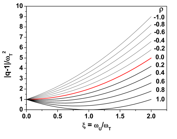
Figure 1: (Color online) Dependence of the ratio $|q-1|/\omega^{2}_{T}$ on the relative fluctuations, $\xi$, for different values of correlation parameter $\rho$.

When $U=const$ (i.e., $\xi=0$) we have the same situation we encountered for a fluctuating temperature, namely that $|q-1|/\omega_{T}^{2}=1$. When we allow energy to fluctuate and add these fluctuations, $|q-1|/\omega^{2}_{T}$ changes as shown in Fig. 1. Notice that condition $q\leq 2$, implies that $\omega_{U}+\omega_{T}\leq 1$, for $\rho\neq 0$, and that $\omega^{2}_{U}+\omega^{2}_{T}\leq 1$ for $\rho=0$ .

3 An application

As an example we compare fluctuations extracted from the distribution of different observables in a high energy multiparticle production process. It should be remembered that Eq. (27) connects fluctuations of different observables, but defined in the same fragment of allowed phase space, whereas available data usually refer to different parts of this phase space. Therefore, corresponding $q$ parameters are usually difficult to compare. For example, $q=q_{L}$ obtained from rapidity ($y$) distributions, $dN/dy$, defined in so-called longitudinal phase space, are comparable with q evaluated from the multiplicity distributions, $P(N)$, which are defined in the full phase space [13, 16]. On the other hand, transverse momentum ($p_{T}$) distributions, $dN/dp_{T}$, defined in the so-called transverse space, are described by much smaller values of $q=q_{T}$. A first attempt to explore the relation (1) in high energy multiparticle production processes was presented in [17].

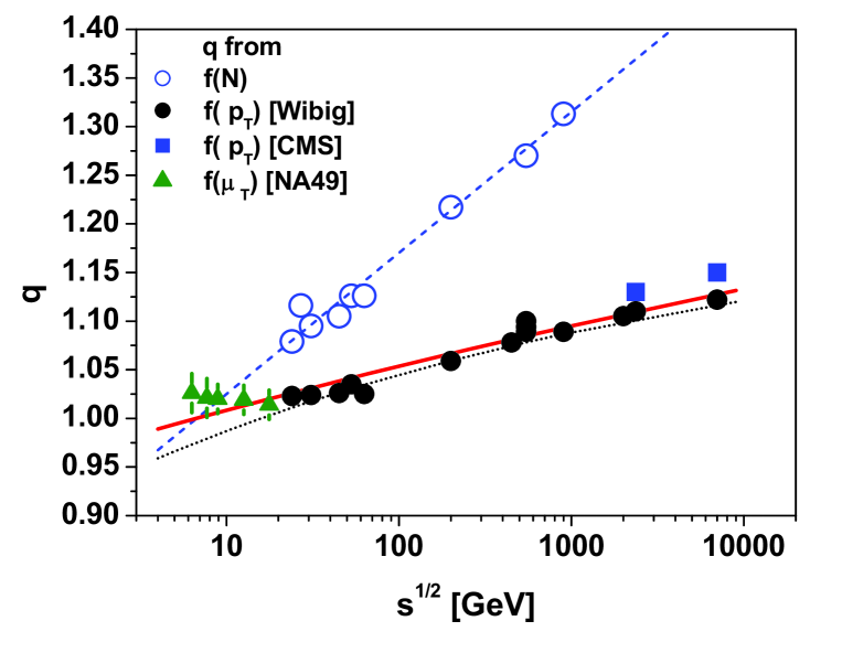
Figure 2: (Color online) An example of energy dependencies of the nonextensivity parameters $q$ obtained from different observables. Open symbols: $q$ obtained from multiplicity distributions $P(N)$ [18] (fitted by $q=1+1/k$ with $1/k=-0.04+0.029\ln s$, cf. [18]). Closed symbols: $q=q_{T}$ obtained from a different analysis of transverse momenta distributions, $f\left(p_{T}\right)$. Data points are from, respectively, [19] for [Wibig], [20] for [CMS] and from [21] (data on $\mu_{T}=\sqrt{m_{\pi}^{2}+p_{T}^{2}}$) for [NA49]). The dotted line represents a fit obtained in [19] ($q_{T}=1.25-0.33s^{-0.054}$) and the full line comes from our Eq. (35).

So far there are no data which would necessitate the use of nonzero correlations. In the case of uncorrelated fluctuations ($\rho=0$ ), one gets from Eq. (27), using (21), that

$$\frac{1}{k}=q-1=\omega^{2}_{U}+\omega^{2}_{T}\,.$$ (32)

In Fig. 2 we plot the energy dependencies of the nonextensivity parameter $q$ obtained from different sources: from the multiplicity distributions, $f(N)=P(N)$, i.e., from the full phase space [18] and from a different analysis of transverse momenta distributions, $f\left(p_{T}\right)$ (i.e., from the transverse phase space [19, 20, 21]). The characteristic feature seen there is that, whereas the former show substantial energy dependence (and essentially follow results for $q=q_{L}$ obtained in [13] from the analysis of $dN/dy$), the latter $q=q_{T}$ are only weakly dependent on the interaction energy (notice also that $q_{T}(s)$ from different sources plotted in Fig. 2 are roughly the same). To somehow compare $q$ and $q_{T}$, one needs some additional input. Assume that, being only weakly energy dependent, $q_{T}$ are also roughly independent of the energy fluctuations. It is now natural to expect that transverse characteristics are mainly governed by the fluctuations of temperature, i.e., that we can write

$$q_{T}-1=\frac{2}{3}\omega^{2}_{T}$$ (33)

(it is assumed here that fluctuations of temperature contribute equally to each of the components of momenta, hence the factor $2/3$). Following this line of thought, i.e., assuming additionally that fluctuations of energy $U$ are entirely given by its thermal part, one can write that in this case $\omega^{2}_{U}=\omega^{2}_{T}$ and that both parameters, $q$ and $q_{T}$, are connected by the following relation:

$$q-1=3\left(q_{T}-1\right)\qquad{\rm or}\qquad q_{T}=\frac{1}{3}(2+q).$$ (34)

A few explanatory remarks are in order. Namely, in [19, 20] the $p_{T}$ distributions were fitted using Tsallis distributions using the power $1/(1-q_{T})$. However, one should keep in mind that in $p_{T}$ distributions one has the prefactor $p_{T}/T^{2}$, not $1/T$, present in the usual exponential distributions. This fact results in a slightly different power, $q_{T}/(1-q_{T})$ [11] (this is the situation similar to the change from the so-called superstatistics A, in which only expression under the exponent is subjected to fluctuations, to superstatistics B, in which one fluctuates also the prefactor [11], cf. also [22]). As a result the relation between $q_{T}$ and $q$ is slightly modified and Eq. (34) now becomes

$$q_{T}=\frac{1+2q}{2+q}.$$ (35)

Using values of $q=1+1/k=0.896+0.029\ln s$ obtained from $P(N)$ [18], the evaluated $q_{T}$ is shown in Fig. 2 (solid line) and compared to $q_{T}$ extracted from transverse momenta distributions $f(p_{T})$ [19, 20, 21]. This, in turn, should be compared with the dotted line representing the fit in [19] resulting in $q_{T}=1.25-0.33s^{-0.054}$. Notice the good agreement of Eq. (35) with data which, in our opinion, justifies the statement that Eq. (35) represents a kind of rule connecting fluctuations in different parts of phase space (modulo additional assumptions).

4 Summary

Using nonextensive statistics applied to ensembles in which the energy ($E$), temperature ($T$) and multiplicity ($N$) fluctuate, we have derived a specific relation connecting all fluctuating variables, Eq. (27), which generalizes Linhard’s thermodynamic uncertainty relation given by Eq. (1). This is illustrated using example taken from the multiparticle production processes. A possibility of connecting fluctuations appearing in different parts of phase space is indicated, cf. Eq. (35).

References

- [1] See: N. Bohr, Collected Works, ed. J. Kalekar (North-Holland, Amsterdam, 1985), Vol. 6, pp. 316-330 and 376-377.
- [2] J. Uffink and J. van Lith, Found. Phys. 29 (1999) 655 and Thermodynamic uncertainty relations, cond-mat/9806102.
- [3] B. H. Lavenda, Found. Phys. Lett. 13 (2000) 487.
- [4] J. Lindhard, ’Complementarity’ between energy and temperature, in The Lesson of Quantum Theory, edited by J. de Boer, E. Dal and O. Ulfbeck (North-Holland, Amsterdam, 1986).
- [5] C. Tsallis, Eur. Phys. J. A 40 257, for an updated bibliography on this subject see http://tsallis.cat.cbpf.br/biblio.htm.
- [6] G. Wilk and Z. Włodarczyk, Phys. Rev. Lett. 84 (2000) 2770.
- [7] T. S. Biró and A. Jakovác, Phys. Rev. Lett. 94 (2005) 132302.
- [8] L. D. Landau and I. M. Lifschitz, Course of Theoretical Physics: Statistical Physics, Pergamon Press, New York 1958.
- [9] L. Stodolsky, Phys. Rev.Lett. 75 (1995) 1044.
- [10] Kulesh Chandra Kar, Phys. Rev. 21 (1923) 672.
- [11] G. Wilk and Z. Włodarczyk, Physica A 376 (2007) 279.
- [12] P. Carruthers and C. S. Shih, Int. J. Mod. Phys. A 2 (1986) 1447.
- [13] F. S. Navarra, O. V. Utyuzh, G. Wilk, and Z. Włodarczyk, Phys. Rev. D 67 (2003) 114002.
- [14] C. Vignat and A. Plastino, Phys. Lett. A 360 (2007) 415.
- [15] V. V. Begun, M. Gaździcki, M. I. Gorenstein and O. S. Zozulya, Phys. Rev. C 70 (2004) 034901. V. V. Begun, M. I. Gorenstein, M. Hauer, V. P. Konchakovski and O. S. Zozulya, Phys. Rev. C 74 (2006) 044903; V. V. Begun, M. Gaździcki, M. I. Gorenstein, M. Hauer, V. P. Konchakovski and B. Lungwitz, Phys. Rev. C 76 (2007) 024902; M. I. Gorenstein, M. Hauer, and D. O. Nikolajenko, Phys. Rev. C 76 (2007) 024901.
- [16] G. Wilk, Z. Włodarczyk and W. Wolak, Composition of fluctuations of different observables, arXiv:1012.1975[hep-ph], to be published in Acta Phys. Polon. B (2011), May issue.
- [17] G. Wilk and Z. Włodarczyk, Phys. Rev. C 79 (2009) 054903.
- [18] A. K. Dash and B. M. Mohanty, J. Phys. G 37 (2010) 025102; see also C. Geich-Gimbel, Int. J. Mod. Phys. A 4 (1989) 1527.
- [19] T. Wibig, J. Phys. G 37 (2010) 115009.
- [20] V. Khachatryan et al. (CMS Collaboration), Phys. Rev. Lett. 105 (2010) 022002 and J. High Energy Phys. 02 (2010) 041.
- [21] C. Alt et al., Phys. Rev. C 77 (2008) 034906; C. Alt et al., Phys. Rev. C 77 (2008) 024903 (2008); S. V. Afanasiev et al., Phys. Rev. C 66 (2002) 054902.
- [22] C. Beck, Continuum Mech. Thermodyn. 16 (2004) 293 and Eur. Phys. J. A 40 (2009) 267.
- [23] M. Nauenberg, Phys. Rev. E 67 (2003) 036114 and Phys. Rev. E 69 (2004) 038102; C. Tsallis, Phys. Rev. E 69 (2004) 038101; R. Balian and M. Nauenberg, Europhysics News 37 (2006) 9; R. Luzzi, A. R. Vasconcellos and J. Galvao Ramos, Europhysics News 37 (2006) 11.
- [24] O. J. E. Maroney, Phys. Rev. E 80 (2009) 061141.
- [25] T. S. Biró, K. Ürmösy and Z. Schram, J. Phys. G 37 (2010) 094027.