The nearest neighbor statistics for X-ray source counts
II. Chandra Deep Field South

Abstract

Context. It is assumed that the unresolved fraction of the X-ray background (XRB) consists of a truly diffuse component and a population of the weak sources below the present detection threshold. Albeit these weak sources are not observed directly, their collective nature could be investigated by statistical means.

Aims. The goal is to estimate the source counts below the conventional detection limit in the Chandra Deep Field-South 2Ms exposure.

Methods. The source number counts are assessed using the nearest neighbor statistics applied to the distribution of photon counts. The method is described in the first paper of these series.

Results. The source counts down to $3-4\cdot 10^{-18}$ cgs in the soft band ($0.5-2$ keV) and down to $2-3\cdot 10^{-17}$ cgs in the hard band ($2-8$ keV) are evaluated. It appears that in the soft band the source counts steepen substantially below $\sim\!10^{-16}$ cgs. Assuming that the differential slope $b\approx 1.5-1.6$ in the range $10^{-16}-10^{-14}$ cgs, the number of weaker sources indicates the slope of $\approx-2.0$. The steepening is not observed in the hard band.

Conclusions. Steepening of counts in the soft band indicates a new population of sources. A class of normal galaxies at moderate redshifts is a natural candidate.

1 Introduction

Source number counts are investigated in one of the deep Chandra pointing, viz. the Chandra Deep Field South (CDFS). An original method based on the nearest neighbor statistics (NNST) has been used. In the first paper (Sołtan, 2010, hereafter SI) we presented the method and demonstrated its efficiency for the source number counts analysis. It was applied to the Chandra exposure of $\sim\!460$ ks in the Groth Strip. The NNST allowed us to determine the $N(S)$ relationship for sources generating merely $\sim\!2$ counts, i.e. roughly an order of magnitude below a standard threshold for a detection of discrete point-like sources. Application of the NNST to the CDFS shifts the sensitivity limit below $4\cdot 10^{-18}$ cgs, in the $0.5-2$ keV band, still a factor of $\sim\!3$ below the present deepest number counts determinations (Georgakakis et al., 2008, hereafter GNL).

A comprehensive discussion of the present method is given in SI. Here only a general framework is sketched. From the point of view of spatial characteristics, the counts collected in the focal plane of the X-ray telescope are arranged into two populations. The first, randomly distributed, includes the X-ray photons generated by a truly diffuse XRB and locally scattered X-rays of various origin as well as the particle background. The weak sources which generate in the exposure exactly one count each also contribute to this category, if they are distributed randomly within the field of view. The second class is generated by the discrete sources producing at least two photons. Counts of this class are distributed in clumps defined by the point spread function (PSF) of the X-ray telescope.

One should expect that a distribution of the nearest neighbors for both classes of counts is different. On the average, the counts produced by sources have closer neighbors than the non clustered counts.

The observed distribution of the nearest neighbors results from the relative contribution of the randomly distributed counts, $n_{1}$, and the number of sources, $N_{k}$, producing $k$ photons each, where $k=2,3,...,k_{\rm max}$, with $k_{\rm max}$ representing the strongest source in the field. The total number of counts is a sum of both constituents:

$$n_{t}=n_{1}+\sum_{k=2}^{k_{\rm max}}k\cdot N_{k}\,.$$ (1)

We define $P(r)$ as the probability that the distance to the nearest neighbor from the randomly picked count is greater then $r$. The relationship between the source population $N_{k}$ and the probability $P(r)$ is given in SI:

$$\frac{n_{1}}{n_{t}}\,P(r|1)\>+\>\sum_{k=2}^{k_{\rm max}}\;\frac{n_{k}}{n_{t}}\;P(r|1)\>{\cal P}(r|k)\>=\>P(r)\,,$$ (2)

where $P(r|1)$ is the probability that the distance to the nearest neighbor from the randomly selected point (not count) exceeds $r$, $n_{k}=k\cdot N_{k}$ is the total number of photons in the field produced by sources generating $k$ photons each, and ${\cal P}(r|k)$ describes the nearest neighbor probability within a cluster of $k$ counts generated by a single source. The probability ${\cal P}(r|k)$ is fully defined by the PSF.

The numbers of sources $N_{k}$ depend on the source number counts $N(S)$. The relationship between the source flux, $S$, and the number of actually detected source counts, $k$, is given by the Poissonian distribution:

$$p(k|S)=\frac{e^{-s}\,s^{k}}{k!}\,,$$ (3)

where $p(k|S)$ is the probability that source with flux $S$ generates $k$ counts, while $s$ is the expected number of counts, or it is the source flux expressed in the units of counts. The flux $s$ in the ACIS counts is related to the flux in physical units, $S$, by:

$$s=S/{\rm cf}\,,$$ (4)

where ${\rm cf}$ is the conversion factor which has units of “erg cm^-2 s${}^{-1}/{\rm count}$” and is related to the parameter “exposure map” defined in a standard processing of the ACIS data. For the real observations, both the cf and exposure map are functions of the position. The present analysis is restricted to the area where the cf variations are small (see below). A question of the cf variations over the field of view is discussed in SI.

For the power law number counts $N(s)=N_{o}\,s^{-b}$, Eq. 2 takes the form:

$$\frac{N_{o}}{n_{\rm t}}\,P(r|1)\sum_{k=2}^{k_{\rm max}}\frac{\Gamma(k-b+1)}{\Gamma(k)}\>\left[1-{\cal P}(r\!\mid\!k)\right]=P(r\!\mid\!1)-P(r)\,.$$ (5)

For different parametrization of the source counts the Eq. 5 could be modified, in particular for the broken power law:

$$N(s)=N_{o}\left(\frac{s}{s_{o}}\right)^{b}\,,\hskip 28.45274ptb=\left\{\begin{array}[]{ccc}b_{1}&\mbox{for}&s\geq s_{o}\\ b_{2}&&s<s_{o}\end{array}\right.$$ (6)

the $\Gamma$ function in the numerator is replaced by the appropriate combination of the incomplete $\Gamma$ functions.

Since we are interested in the distribution of weak sources, all the discrete sources strong enough to be isolated using the standard methods should be extracted from the observations. After the removal of bright sources, the $k_{\rm max}$ value corresponds to the weakest sources which could be unmistakably recognized as individual objects. In derivation of Eq. 5 it is assumed also that the exposure is sufficiently deep to use the functional form of $N(s)$ rather than the actual number of sources $N_{k}$.

A standard method to estimate the number counts of weak sources is based on the fluctuation analysis. The sources in the observation area increase fluctuations of the count number in the detection cell above that expected for the Poissonian distribution. The fluctuation enhancement is dominated by the strongest sources, while it is very weakly affected by the faint sources which contribute only a few counts. This is because the fluctuations amplitude is related to the second moment of the count distribution.

The NNST weights the contribution of weak and strong sources more evenly: a deviation from the random distribution defined as the right-hand side of Eq. 5 depends linearly on the number of counts $n_{k}$. Thus, the NNST appears to be a relatively sensitive tool to quantify the contribution of counts produced by weak sources and can be efficiently applied to assess the $N(S)$ relationship at the low flux end.

The organization of the paper is as follows. In the next section the observational material is described and the computational details including questions related to the PSF are given. Results of the calculations, i.e. estimates of the source counts below the nominal sensitivity limit in the CDFS are presented in Sect. 3. The results are summarized and discussed in Sect. 4.

2 Observational material

In the present paper we analyze the counts collected in the Chandra ACIS-I chips 0 - 3. The CDFS was observed with the ACIS detector in several ”sessions”. Although the observations span a period of more than $7$ years, the data have been processed in a uniform way with the recent pipeline processing versions. The details of $20$ observations used in the present paper are given in Table 1. All the exposures have been scrutinized with respect to the background flares and only the “good time intervals” were used in the subsequent analysis. The data have been split into two energy bands: S – soft ($0.5-2$ keV) and H – hard ($2-8$ keV).

Table 1: Log of the CDFS observations used in the paper

Obs.	Observation and processing		Processing	Exposure
ID	dates		version	time [s]
441	2000-05-27	2007-05-23	7.6.10	56600
582	2000-06-03	2007-05-23	7.6.10	132150
2405	2000-12-11	2007-06-20	7.6.10	57100
2312	2000-12-13	2007-06-20	7.6.10	125100
1672	2000-12-16	2007-06-20	7.6.10	96150
2409	2000-12-19	2007-06-21	7.6.10	69850
2313	2000-12-21	2007-06-22	7.6.10	131900
2239	2000-12-23	2007-06-22	7.6.10	132600
8591	2007-09-20	2007-09-21	7.6.11.1	45800
9593	2007-09-22	2007-09-27	7.6.11.1	46100
9718	2007-10-03	2007-10-06	7.6.11.1	49850
8593	2007-10-06	2007-10-08	7.6.11.1	49250
8597	2007-10-17	2007-10-24	7.6.11.2	59650
8595	2007-10-19	2007-11-07	7.6.11.2	116850
8592	2007-10-22	2007-11-01	7.6.11.2	87750
8596	2007-10-24	2007-11-14	7.6.11.2	116600
9575	2007-10-27	2007-11-14	7.6.11.2	110150
9578	2007-10-30	2007-11-30	7.6.11.2	39000
8594	2007-11-01	2007-11-14	7.6.11.2	143300
9596	2007-11-04	2007-11-20	7.6.11.2	116600
			Total exposure  1782350

Table 2: Energy bands and conversion factors

Energy band		Conversion factors†
[keV]		Average	rms	minimum	maximum
S	$0.5-2$	$3.701$	$0.205$	$3.232$	$4.218$
H	$2-8$	$14.30$	$0.85\leavevmode\nobreak\$	$12.69$	$16.28$
† The conversion factor (cf) has units of $10^{-18}\,{\rm erg\,cm}^{-2}\,{\rm s}^{-1}/{\rm count}$.

2.1 The exposure map

The observations, listed in Table 1 were merged to create a single count distribution and exposure map. A circular area covered by all the pointings with a relatively uniform exposure, centered at ${\rm RA}=3^{\rm h}32^{\rm m}$, ${\rm Dec}=-27\deg 49\arcmin$ with radius of $5\aas@@fstack{\prime}0$ in the S band and $4\aas@@fstack{\prime}0$ in the H band has been selected for further processing. The exposure map of the individual observation resulting from various instrumental characteristics has a complex structure. The exposure map of the merged observation exhibits significant variations too, although it is more uniform than the individual components. To reduce further the variations of the exposure map over the investigated area, a threshold of the minimum exposure has been set separately for both energy band. Pixels below this threshold have not been used in the calculations.

A threshold has been defined at $77$ % of the maximum value of the exposure map in the S band and $78$ % in the H band. As a result, in both energy bands the maximum deviations of the exposure from the average value do not exceed $15$ % and the exposure rms over the investigated areas fall below $6$ %. In Table 2 the conversion factors corresponding to the relevant amplitudes of the exposure maps are given. In the calculations “from counts to flux” a power spectrum with a photon index $\Gamma_{\rm ph}=1.4$ was assumed (Kim et al., 2007).

Variations of the conversion factor, ${\rm cf}$, over the investigated area alter the source fluxes via Eq. 4 and, consequently, the source counts $N(S)$. However, it is shown in SI that in the linear approximation variations of the exposure maps and the conversion factor do not affect the probability distributions $P(r\!\mid\!1)$ and $P(r)$. Thus, the restrictive limits imposed on the cf fluctuation amplitude ensure that the NNST should yield reliable results.

2.2 The count selection

A single cosmic ray can induce in the ACIS CCD detector a series of $2$ or more “events”. This well recognized feature, known as “afterglow”, generates spurious weak sources in the data and potentially could affect the present investigation. Fortunately, as indicated in SI, the afterglow counts span short time intervals as compared to the exposure times of all the observations. The material has been scrutinized with respect to the afterglows and events identified with that phenomenon have been removed from the observation.

Strong sources were localized in the field using the Giacconi et al. (2002) catalog based on 1Ms exposure. Around each cataloged source position a radius $r_{85}$ encircling $85$ % of the point source counts has been calculated using the local PSF parameters (see below). Then, number of counts within $r_{85}$ was obtained, and - by subtracting the background counts - the net counts $k_{85}$ were assessed for the each source. Since the relative variation of the exposure within the field of view (fov) are small, the average background was assumed for the entire field. The threshold counts $k_{\rm max}$ characterizing the completeness limit of the catalog is not well defined, and a range of $k_{\rm max}$ between $20$ and $45$ were applied in the analysis in both energy bands. For given $k_{\rm max}$, the source has been excluded from further processing if $k_{85}>0.85\cdot k_{\rm max}$. To assure the removal of the source counts in the PSF wings, the rejection area was a circle with radius $r_{\rm rem}=4\cdot r_{85}+4\arcsec$.

In the standard processing of the ACIS data the discrete pixel coordinates are randomized over the square pixel size of $0\aas@@fstack{\prime\prime}492$ a side. Accordingly, the count separations are subject to randomization at the pixel size scale. To assess the effect of randomization on the NNST probability distributions, a set of $12$ “observational“ data was generated by randomization of count position within pixels using the original event files with non-randomized (integer) count coordinates.

2.3 The Point Spread Function

The ${\cal P}(r|k)$ probability has been calculated by means of the Monte Carlo method using the model PSF. The procedure to construct the PSF suitable to the present investigation is described in details in SI.

Figure 1: Encircled count fraction (ECF) in the S band as a function of a distance from the count centroid. Example distributions are shown for $2$ sources at $2\aas@@fstack{\prime}1$ and $5\aas@@fstack{\prime}9$ from the field center. Solid curves – the observed count distributions, dashed curves – fits obtained using Eqs. 7 and 8, dotted curves – the ECF distributions differing from the best fit by $\pm 15$ %.

Figure 2: Same as Fig. 1 for the H band.

The Chandra X-ray telescope PSF is a complex function of source position and energy (e.g. Allen et al., 2004). To compute the ${\cal P}(r|k)$ probability which describes the nearest neighbor distribution in the entire data set, we need to generate the PSF appropriately averaged over the field of view. A tractable method to obtain the ${\cal P}(r|k)$ was to find an analytic approximation for the encircled count fraction (ECF) for a point source as a function of the distance from the field center. To reproduce the count distribution for a single source, we have used the function of the form

$$ECF(<r)=\frac{r^{\alpha}}{z+r^{\alpha}+y\cdot r^{\alpha/2}}$$ (7)

with free parameters $\alpha$, $z$, and $y$. A shape of the PSF depends strongly on the distance from the optical axis of the telescope. For a single observation the optical axis is shifted from the geometrical center of the ACIS chips 0 - 3. However, in the merged data of $20$ pointings the axis appropriate for the PSF modeling is not well defined and it was assumed that the variations of the PSF shape are symmetrical with respect to the fov center. By fitting the $\alpha$, $z$, and $y$ to the ECF distributions of a number of sources scattered over the entire fov it was found that variations of these parameters can be conveniently parametrized by the distance from the field center $\theta$. It was assumed that:

$$\alpha=a_{\alpha}\cdot\theta+b_{\alpha}\\ y=a_{y}\cdot\theta+b_{y}\\ \log z=a_{z}\cdot\theta+b_{z}\,,$$ (8)

where $a_{s}$ and $b_{s}$ ($s=\alpha$, $y$, $z$) are six parameters which are substituted in Eq. 7 and simultaneously fitted to the observed distribution of counts in the several dozen strongest sources.

In Figs. 1 and 2 examples of the resultant fits to the observed distribution are shown in both energy bands. Although the fitting procedure provides sensible and functional representation of the PSF over the fov, it is difficult to assess the impact of the potential systematic errors generated by the present approximation on our final results. To control the systematics, we have constructed two model ${\cal P}(r|k)$ distributions using the ECF functions systematically wider and narrower by $15$ % as compared to the best fit.

Examples of the ECFs differing from the best fit by $15$ % are shown in Figs. 1 and 2 with the dotted curves. Albeit deviations of individual fits are quite large, the $\pm 15$ % ECF envelopes undoubtedly encompass the systematic errors produced by Eqs. 7 and 8.

In the Monte Carlo computations of ${\cal P}(r\!\!\mid\!\!k)$ a population of $10^{8}$ “sources” of $k=2,3,...,k_{\rm max}$ counts were distributed randomly over the investigated area. The distribution of counts within each source was randomized according to the model ECF. Then, for each source a distribution of the nearest neighbor separations was determined and used to obtain the corresponding amplitudes of ${\cal P}(r\!\!\mid\!\!k)$. The procedure has been executed for the best fit and $\pm 15$ % ECF distributions.

In Fig. 3 the probability densities based on the integral distributions ${\cal P}(r\!\!\mid\!\!k)$ in the S band are shown for several values of $k$. To visualize more clearly details of the relevant distributions, probability densities, i.e. $|d{\cal P}(r|k)/dr|$ rather than ${\cal P}(r\!\!\mid\!\!k)$ are plotted. The dashed curve shows the probability density of the nearest neighbors distances for the random distribution.

Figure 3: The probability density of the distance to the nearest neighbor in the S band for counts produced by sources generating $k=2$, $4$, $10$, and $20$ counts. The dashed curve shows the expected distribution for the pure random count distribution.

Conspicuously, due to a high average count density, the nearest neighbor of the photon generated by the sources producing $k=2$ counts, is less likely to originate from the same source rather than to be a chance coincidence with the unrelated event. It shows the natural limitations of the method. The NNST can be efficiently used for the investigation of the weak sources if they are sufficiently numerous to significantly modify the number of the nearest neighbors observed for the random distribution.

3 The source counts

3.1 The soft band

Using the selection criteria given in Sect. 2, the accepted area and the total number of counts in the soft band amount to to $71.8$ sq. arcmin and $158\,795$, respectively. After the removal of strong sources according to the procedure described above, the area is reduced to $66.5$ sq. arcmin and the number of counts to $110\,996$ for $k_{\rm max}=45$ and to $65.4$ sq. arcmin and $108\,778$ counts for $k_{\rm max}=30$. The average density of counts amounts to $\sim 0.463$ per sq. arcsec. and the average distance to the nearest neighbor for the random distribution is equal to $0\aas@@fstack{\prime\prime}736$.

All the calculations have been performed in a similar way as in SI. The nearest neighbor distributions were calculated separately for $12$ data sets obtained by randomization of events within pixels. Analogously, the distribution of distances between the random points and the data were obtained. Then, these distributions were used to calculate the $P(r)$ and $P(r|1)$ probabilities. Taking advantage of a wide range of separations $r$ over which the probability distributions were determined, Eq. 5 was rewritten using the differential probability distributions $\Delta P(r)=P(r)-P(r+\Delta R)$ (and $\Delta P(r|1)$ alike). Accordingly, the Eq. 5 has been replaced by a set of equations for the consecutive values of $r$ and the best estimate of the slope $b$ was found by minimizing the $\chi^{2}$ of the fit. In our calculations we used the separations range $0<r<2\arcsec$ and $\Delta r=0\aas@@fstack{\prime\prime}1$.

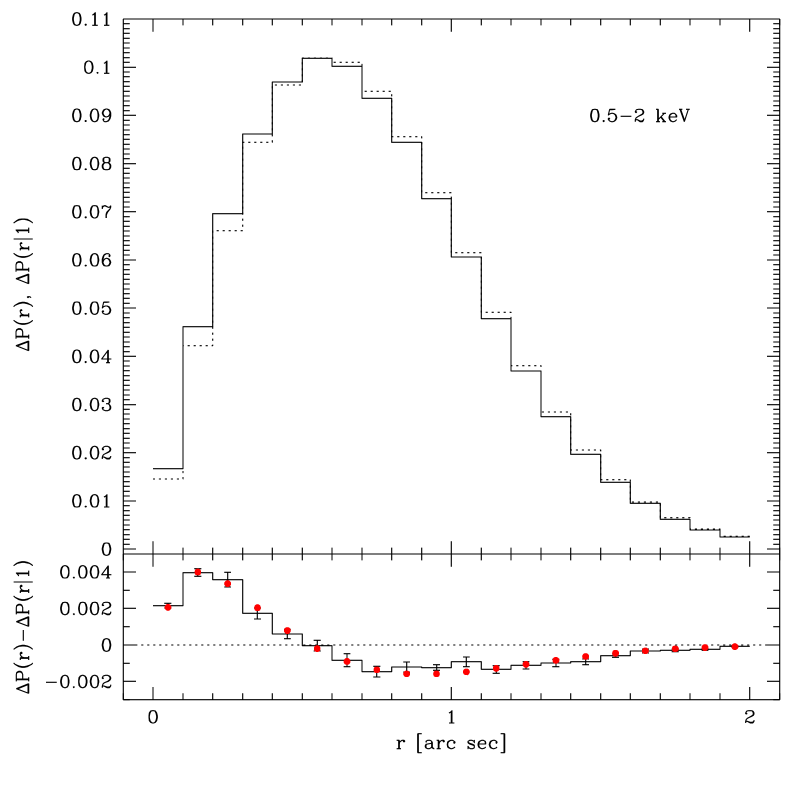
Figure 4: Upper panel: the nearest neighbor probability distributions binned with $\Delta r=0\aas@@fstack{\prime\prime}1$ for the observed counts (solid histogram), and between random points and the observed counts (dotted histogram). Lower panel: the difference between both distributions; the error bars show $1\sigma$ uncertainties; dots - the best fit (see text for details).

Previous investigations of the deep Chandra fields, e.g. Kim et al. (2007) and GNL, provide essentially consistent assessments of the $N(S)$ counts above the detection threshold for the discrete sources. In particular, in the interesting flux range GNL approximate the number counts by a power law with the slope of $-1.58$. To conform the present investigation to the observed counts at the bright end, we assume that the $N(s)$ relationship defined in Eq. 6 above $s_{o}=20$ counts matches exactly the GNL model. Thus, the only parameter to be determined using the set of equations generated by Eq. 6 is the slope $b_{2}$ at the low flux end.

In the upper panel of Fig. 4 the probability distributions $\Delta P(r)$ and $\Delta P(r|1)$ are shown for $k_{\rm max}=40$. The $\Delta P(r)$ histogram is the average of of $12$ realizations of the pixel randomization routine. The difference of both distributions is shown in the lower panel. The error bars represent the rms scatter between $12$ randomized observations. The dots show the average of $12$ best fit solutions obtained using the NNST. The analogous distributions constructed for several values of $k_{\rm max}$ between $20$ and $45$ provided qualitatively similar results.

Flux $s_{o}=20$ counts marking the slope change corresponds to $S=7.84\cdot 10^{-17}$ cgs. The best fit slope below the power law break $b_{2}=-2.02^{+0.11}_{-0.08}$, where the errors represent $1\sigma$ statistical uncertainties (for the full discussion of uncertainties see below). This result is compared in Fig. 5 with the source counts presented by GNL and our recent estimate in SI based on the shallower exposure in the AEGIS field.

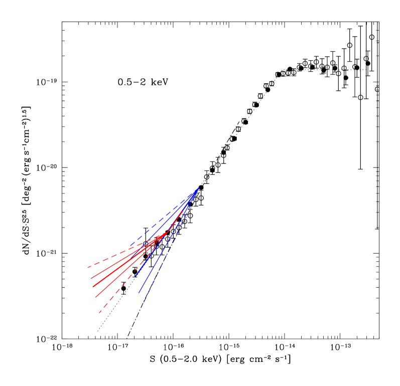
Figure 5: Differential number counts in the $0.5-2$ keV band normalized to the Euclidean slope. The data points and the dotted line are taken from Georgakakis et al. (2008); dot-dash curve shows the AGN model by Ueda et al. (2003). The right bundle of lines exiting from the point at $S=3\cdot 10^{-16}$ cgs represents the solution obtained in SI based on the pointing at the AEGIS field; the left bundle shows the present results based on CDFS: thick line - the best fit solution, thin lines - $1\sigma$ statistical uncertainty, dashed lines - maximum total uncertainty range including the potential systematic errors generated by the approximations in the PSF fitting.

The data points in Fig. 5 are based on a large number of Chandra pointings, including CDFS. The full dots in Fig. 5 show the GNL measurements and the open circles – the Kim et al. (2007) results. Over a wide flux range the GNL counts in fact follow the power law with the slope $-1.58$. Below the flux $S\approx 6\cdot 10^{-17}$ cgs GNL notice that the number counts seem to be steeper, though the deviation from the power law is rather modest. In the range of $6\cdot 10^{-17}-3\cdot 10^{-16}$ cgs, the number counts determined by Kim et al. (2007) run slightly below the GNL data.

Solid and dashed lines covering fluxes between $\sim 2\cdot 10^{-17}$ and $3\cdot 10^{-16}$ cgs are taken from SI and show the best fit and the statistical uncertainty as well as the total uncertainties. The present investigation covers the flux range of $\sim 3\cdot 10^{-18}-1.5\cdot 10^{-16}$ cgs and in Fig. 5 is represented by the best solution line and lines defining the uncertainty ranges (see below).

The SI solution in a good agreement with both the GNL and Kim et al. (2007) data. Although, the SI estimate are consistent with the results available in the literature, the relevant slope uncertainties are uncomfortably high and do not constrain strongly the $N(S)$ relationship. The present results also are not highly restrictive. Nevertheless, the acceptable slopes seem to be distinctly steeper than those by GNL.

3.2 Error estimates

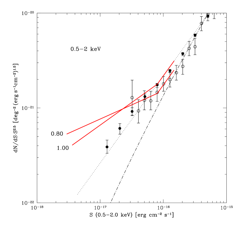
Figure 6: Low flux end of the differential number counts in the $0.5-2$ keV band normalized to the Euclidean slope. The data points, the dotted and dot-dash curves as in Fig. 5. Broken solid lines: the NNST solutions for the $N(S)$ with the bright end normalization according to Georgakakis et al. (2008) - label ”$1.00$”, and the normalization reduced by $20$ % - label ”$0.80$”.

The best estimates of slope in SI and the present results are shown with the thick solid lines. The uncertainties introduced by the statistical character of the nearest neighbor method are indicated by the thin lines. These uncertainties result from variations of the nearest neighbor probability distributions produced by the randomization of counts within pixels .

The systematic errors affecting the investigation are probably dominated by the inaccuracies in the calculations of the ${\cal P}(r|k)$ probabilities. These uncertainties have been accounted for using the “extreme” ECF functions described in the Sect. 2.3. A set of $12$ solutions has been obtained using the ${\cal P}(r|k)$ distribution derived from each of the side ECF. Then, the average values of the slope and the respective rms amplitudes in both sets were calculated. The dashed lines in Fig. 5 show the uncertainty range implied by these calculations, assuming the joint effect of the systematic errors and the rms scatter. This estimate of the “total” error is highly conservative. It is obtained by simple addition of statistical uncertainty and the systematic errors assuming their highest “reasonable” values.

A question of the exposure variations over the fov is discussed in SI. For the power law counts, variations of the exposure map generate errors in the $N(S)$ which one can express as variations of the count normalization $N_{o}$. It is shown that constraints imposed in our investigation on the amplitude of the exposure map variations strongly restrict the magnitude of the equivalent fluctuations of $N_{o}$. In effect, the small exposure map variations do not introduce substantial systematic uncertainties of the slope determination.

Equation 5 explicitly involves both parameters which define the source counts: the slope $b$ and the normalization $N_{o}$. In our calculations only the slope was estimated while the normalization was fixed. Still, one can obtain a formal solution for those parameters. Unfortunately, the best estimates of $b$ and $N_{o}$ found by a simultaneous fitting are highly correlated. This is because the NNST is affected predominantly by the total number of close pairs. Thus, a quality of the fit depends on the proper combination of $b$ and $N_{o}$, rather than on each parameter separately. In Fig. 6 two best fit solutions are shown for two different bright end normalization $N_{o}$. The broken line labeled ”$1.00$” is the same as in Fig. 5, while the line labeled ”$0.80$” shows the counts with the $N_{o}$ reduced by $20$ %.

3.3 The hard band

The NNST is basically used to calculate the excess of the close photon pairs as compared to the number of pairs expected for the random distribution. High overall count density in the $2-8$ keV band significantly limits the efficiency of the NNST method for the weak source investigation. After the removal of strong sources, the average distance to the nearest neighbor for the random distribution amounts to just $0\aas@@fstack{\prime\prime}51$ and the NNST applied to the $5\arcmin$ radius fov has not produced any meaningful constraints on the $N(S)$ slope.

In order to improve the S/N ratio we confined our calculations to the central area of $4\arcmin$ radius where the PSF is relatively narrow. The total number of counts within this limited field amounts to $179371$. After the removal of sources generating more than $k_{\rm max}=40$ the number of counts is reduced to $144632$. Our slope estimate and its statistical uncertainty $b=-1.23^{+2.28}_{-0.53}$ are consistent with the available source counts. Unfortunately, the constraints imposed on $N(S)$ still are not restrictive, particularly the lower slope limit is insignificant. Nevertheless, the NNST rather strongly excludes any substantial steepening of the counts, contrary to the result obtained for the S band. This is shown in Fig. 7, where the present results are confronted with the available observational material. The points with the error bars are drawn using the $2-10$ keV data presented by GNL. The power spectrum with a photon index of $-1.4$ was assumed to convert fluxes from the $2-10$ keV band to our H band. The NNST solution and $1\sigma$ statistical uncertainties are shown with the solid thick line and two thin lines, respectively. The dashed lines indicate the combined effect of the maximum potential systematic errors and the statistical noise. The systematic errors have been assessed in a similar way as in the S band. The width of the best fit PSF was altered by $\pm 15$ % to accommodate for conceivable systematic deviations of the analytic fits from the actual PSF (see Fig. 2). Then, the new ${\cal P}(r|k)$ probabilities, based on the modified PSFs, were derived and used in the subsequent calculations.

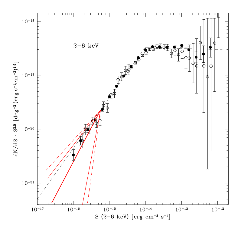
Figure 7: Differential number counts in the $2-8$ keV band normalized to the Euclidean slope. The data points and the dashed line are constructed using the $2-10$ keV band from Georgakakis et al. (2008); the thick solid line - the best fit solution, thin lines - $1\sigma$ statistical uncertainty range, dashed lines - maximum total uncertainty range including the potential systematic errors generated in the PSF fitting.

3.4 Discussion

Our slope estimate below $S\approx 7\cdot 10^{-17}$ cgs is substantially steeper than the recent estimates by GNL. Although these authors also observe the steepening of counts at the lowest attainable flux levels, their slope change is distinctly smaller and the discrepancy between our results remains unexplained. Both the NNST and the GNL approaches make full use of the Poissonian character of the count distribution produced by the individual source. Nevertheless, both methods are distinctly different. GNL assess the source presence by counting the events within the detection cell, while here we analyzed the NN distances between the events. The NNST method has been tested in SI, but it should be considered still as a new tool, and one cannot exclude that unrecognized systematic errors have influenced the present result. Hopefully, the recent Chandra 4Ms observation of the CDFS would help to clarify this question.

The integral source counts are constrained by the amplitude of the extragalactic XRB component. A varying galactic contribution to the total signal makes the estimates of the extragalactic part in the S band somewhat uncertain. As a reference figure we adopt the XRB assessment by Moretti et al. (2003) of $f_{S}=(7.53\pm 0.35)\cdot 10^{-12}$ erg s^-1cm^-2deg^-2. The counts described by the GNL model integrated above $S=7.5\cdot 10^{-17}$ cgs ($\equiv 20$ counts in the present investigation) generate $\sim\!78$ % of the XRB. Using our slope best estimate of $b=2.02$, sources producing $2\leq k\leq 20$ counts contribute further $10$ %. Assuming that the point-like sources generate the whole extragalactic XRB, the $N(S)$ counts should flatten for $S\la 4\cdot 10^{-20}$ cgs. If some fraction of the soft XRB is attributed to the diffuse component, such as the WHIM, the counts flattening has to occur at higher flux levels. In particular, if the WHIM generates $10$ % of the XRB (Sołtan, 2007), the source counts cannot continue with the same slope below $\sim\!2\cdot 10^{-18}$ cgs. Apparently, even the modest extension of the $N(S)$ relationship supplemented with the precise measurements of the integrated XRB would provide a valuable data for the investigation of the diffuse component.

In the S band neither the GNL nor our results are consistent with the predicted counts of AGNs based on a wide class of evolutionary models (e.g. (Miyaji et al., 2000), Gilli et al. (2001), Ueda et al. (2003)). Consequently, a new population of objects emerging below $\sim 10^{-16}$ cgs is required.

Young and/or starburst galaxies appear as a natural candidates for such sources. The XRB spectrum between $1$ keV and $\sim\!20$ keV is adequately approximated by a power law with a photon index of $1.4$ (De Luca & Molendi (2004), and references therein). Below $1$ keV the conspicuous XRB softening is observed (Gilli et al., 2001). The soft excess varies from field to field and evidently exhibits some local and Galactic contribution (e.g. (Markevitch et al., 2002)). However, the fraction of the soft XRB generated within the Galaxy is not well established (Sołtan, 2007). Consequently, the exact spectral characteristics of the extragalactic XRB are not satisfactorily determined.

A question of the discrete source contribution to the diffuse background in the radio domain is also present in the literature. It is interesting that the extragalactic radio source counts exhibit pronounced slope variations of a character resembling those observed in the soft X-rays (see Vernstrom et al. (2011) for the compilation of the radio data). The counts derived from the VLA-COSMOS survey at $1.4$ GHz Bondi et al. (2008) above $\sim 0.5$ mJy indicate the slope of $-1.6$, while just below that flux the slope is equal to $\sim-2.3$. The counts decline again below $\sim 0.1$ mJy.

In the H band the NNST provides consistent results with the previous investigations and the source counts do not exhibit any measurable steepening. It indicates, that the weak sources generating the count rise in the S band have soft spectra and their contribution to the XRB above $2$ keV is low.