Abstract

We propose an organizing principle for classifying and constructing Schrödinger-invariant solutions within string theory and M-theory, based on the idea that such solutions represent nonlinear completions of linearized vector and graviton Kaluza-Klein excitations of AdS compactifications. A crucial simplification, derived from the symmetry of AdS, is that the nonlinearities appear only quadratically. Accordingly, every AdS vacuum admits infinite families of Schrödinger deformations parameterized by the dynamical exponent $z$. We exhibit the ease of finding these solutions by presenting three new constructions: two from M5 branes, both wrapped and extended, and one from the D1-D5 (and S-dual F1-NS5) system. From the boundary perspective, perturbing a CFT by a null vector operator can lead to nonzero $\beta$-functions for spin-2 operators; however, symmetry restricts them to be at most quadratic in couplings.

This point of view also allows us to easily prove nonrenormalization theorems: for any Sch($z$) solution of two-derivative supergravity constructed in the above manner, $z$ is uncorrected to all orders in higher derivative corrections if the deforming KK mode lies in a short multiplet of an AdS supergroup. Furthermore, we find infinite classes of 1/4 BPS solutions with 4-,5- and 7-dimensional Schrödinger symmetry that are exact.

1 Introduction

Since the early days of bottom-up Galilean holography [1, 2], various techniques have been developed to embed Schrödinger solutions into string theory and M-theory. The TsT transformation, or Null Melvin Twist, has been used to transform the asymptotics of various black brane solutions [3, 4, 5, 6, 7, 8, 9], and zero temperature solutions have been embedded into consistent truncations of type IIB and eleven-dimensional supergravities that retain massive vector modes, thereby making contact with the original bottom-up approach [10, 11, 12, 13, 14, 15, 16, 17]. More general solutions, formed directly in $D=10,11$, engineer non-relativistic conformal symmetry geometrically, drawing a connection between harmonic modes on internal manifolds and zero temperature Schrödinger solutions with infinite spectra of $z$, e.g. [18, 19, 20, 21, 22, 23, 24, 25].

For extremal solutions, the construction of [20] is the most general to date. Building on their own work [19] and followed by [21], the authors’ framework subsumes all previously found zero temperature embeddings based on null deformations of the near-horizon D3 and M2-brane solutions, realizing them as members of infinite families of Schrödinger solutions. The spectrum of $z$ is determined by the spectrum of harmonics on Sasaki-Einstein manifolds. The geometric nature of these solutions suggests an extension to other deformations of AdS vacua with some generality.

Given these developments, the outstanding question is no longer how top-down Schrödinger solutions can be found, but instead, what the fundamental principle is that allows us to explain their existence and classify them. In this work, largely inspired by [18, 20, 22], we attempt to answer the following question: given an AdS$\,\times\,\mathcal{M}$ solution, can it always be deformed to have Schrödinger symmetry? The answer, we argue, is yes.

We begin by elucidating and extending the constructions of [18, 20, 22], which stand in direct correspondence to linearized Kaluza-Klein vectors and gravitons of AdS compactification spectra. In fact, we show that this is more than a parallel. To every such spin-2 excitation, there exists a nonlinear solution with Schrödinger symmetry that is obtained by “turning on” the KK mode; and in rather general circumstances, there are Schrödinger solutions that involve both vector and spin-2 excitations which couple only at quadratic order.

The obvious puzzle is why linearized solutions can be extended to nonlinear order in such a simple way. We use perturbation theory around a generic AdS$\,\times\,\mathcal{M}$ vacuum to show that the nonlinearities are constrained by symmetry to arise only at second order. Scale invariance consistent with the first-order solutions determines the geometry to be of Schrödinger form. Putting this all together, for every AdS$\,\times\,\mathcal{M}$ vacuum in string and M-theory, there are Schrödinger solutions in direct correspondence with vector and graviton KK modes of the compactification spectra on $\mathcal{M}$. The most general Schrödinger solutions, which exist when the harmonic spectra on $\mathcal{M}$ admit solution of a simple set of Laplace equations, superpose these modes.

In this sense, the existence of Schrödinger solutions is universal, and their construction, mechanical. We support our arguments by providing three new categories of solutions explicitly, with three-, four- and seven-dimensional Schrödinger symmetry. This includes both supersymmetric and non-supersymmetric solutions.

We also provide an argument on the CFT side. The dual version of the quadratic truncation of the AdS perturbation theory is that the $\beta$-function equations for all deforming operators truncate at second order in the couplings, modulo some issues regarding the effect of multi-trace operators. When perturbing the theory by a source for a null vector operator, scale invariance is preserved provided that no marginal spin-2 operator appears in the OPE of two vector operators. Further parallels can be drawn by considering the Wilsonian $\beta$-functions equations for a tower of spin-2 operators. Their $\beta$-function equations are again constrained by symmetry to be quadratic in the couplings, and the non-relativistic fixed point is easily solved in terms of operator dimensions and constants arising from OPEs between vector operators. This is particularly useful in light of recent work in setting up the precise holographic dictionary for Schrödinger gauge/gravity duality, which focused primarily on solutions to massive vector theories [26, 27]. But the most general embeddings of the type analyzed in this work do not fit into that framework: there are not only massive vectors but massive gravitons as well, dual to symmetric tensor operators with nontrivial Wilsonian $\beta$-functions.

This perspective has powerful implications for the existence of the Schrödinger backgrounds beyond the two-derivative approximation, first considered in [28]. In particular, we recall that conformal dimensions of operators in short multiplets of an AdS supergroup, which are determined via harmonics of $\mathcal{M}$, are unrenormalized by quantum and stringy corrections. This implies that any parameter of a Schrödinger solution that derives from the dimensionless AdS mass of a KK mode can be so protected. This is the case for the dynamical exponent, $z$. Furthermore, when we perturb the exact AdS vacua that arise in the near-horizon limit of M2, D3 and M5 branes, certain infinite families of the resulting Schrödinger solutions are uncorrected to all orders in a higher-derivative expansion of the action. These vacua preserve only eight Poincaré supersymmetries, and constitute a new contribution to the small set of exact solutions of string and M-theory. We back this claim with an explicit calculation showing that one such class of Sch₅ solutions of type IIB is unrenormalized to $O(\alpha^{\prime 3})$, inclusive of all correction terms, known [29] and unknown.

We briefly note that all of our arguments – in particular, the truncation of the perturbation theory at quadratic order – neglect possible effects of multi-trace operators, which appear to play no role in the present context in the large $N$ limit. The existence of classical Schrödinger solutions is apparently robust against effects of operators of spin greater than two. Scale-invariance may be lost upon including $1/N$ effects, but we do not consider this issue here.

The rest of this paper is organized as follows. Section 2 reviews the Schrödinger solutions of type IIB obtained by a D3-brane deformation, and generalizes them with the perturbation theory arguments detailed above, both in the bulk and on the boundary. We also consider the implications for embedding Schrödinger solutions in consistent truncations with massive modes. Section 3 posits conditions for nonrenormalization. Section 4 presents the new Schrödinger constructions, details of which are in the appendices, and section 5 concludes with a discussion.

Note added, v2: Appendix A now presents another infinite family of solutions with seven-dimensional Schrödinger symmetry obtained through deformation of the extended M5 brane geometry that does not lie in obvious correspondence with massive KK modes found in the compactification on AdS${}_{7}\times M_{4}$, as well as a single solution with six-dimensional Lifshitz symmetry with the same general structure as those Lifshitz solutions of [30, 31].

2 Infinite families of Schrödinger solutions from every AdS

In reviewing the type IIB solutions of [18, 20, 22], we emphasize how their structure parallels that seen in the harmonic analysis of the Kaluza Klein spectrum on AdS${}_{5}\times SE_{5}$. We then show that infinite towers of Schrödinger solutions are guaranteed to exist, for any AdS vacuum, and are governed by the structure of the KK towers of massive vectors and gravitons. For convenience, we use the notation and supergravity conventions of [20], the latter of which are found in [32].

2.1 Review and motivation

The type IIB solutions of [20] are

$$\begin{split}ds^{2}&=\Phi^{-1/2}\left(2dx^{+}dx^{-}+h(dx^{+})^{2}+2Cdx^{+}+d\textbf{x}^{2}\right)+\Phi^{1/2}ds^{2}(CY_{3})\\ F_{5}&=dx^{+}\wedge dx^{-}\wedge dx_{1}\wedge dx_{2}\wedge d\Phi^{-1}+\star_{CY_{3}}d\Phi\\ &\quad-dx^{+}\wedge\left(d(\Phi^{-1}C)\wedge dx_{1}\wedge dx_{2}-\star_{CY_{3}}dC\right)\\ G_{3}&=dx^{+}\wedge W\\ \end{split}$$ (2.1)

This solution is a deformed version of D3-branes sitting at the tip of a $CY_{3}$ cone. $\Phi$ and $h$ are functions; $C$ is a one-form; and $W$ is a complex two-form; all of which are defined on $CY_{3}$. The axion-dilaton is set to zero, and $\textbf{x}=(x_{1},x_{2})$. The field equations evaluated on this ansatz reduce to

$$\begin{split}\nabla^{2}_{CY_{3}}\Phi=0\\ d\star_{CY_{3}}dC=0\\ dW=d\star_{CY_{3}}W=0\\ \nabla^{2}_{CY_{3}}h=-|W|^{2}_{CY_{3}}\end{split}$$ (2.2)

where $|W|^{2}_{CY_{3}}$ is the real square of $W$ with indices contracted with the $CY_{3}$ metric. The first of these equations is the usual harmonic condition on $\Phi$, which we use to zoom into the near-horizon region by making the substitution $\Phi=r^{-4}$, and writing the $CY_{3}$ as a cone over a Sasaki-Einstein space $SE_{5}$ as

$$ds^{2}(CY_{3})=dr^{2}+r^{2}ds^{2}(SE_{5}).$$ (2.3)

Upon substitution, we can satisfy the remaining three equations by taking

$$\begin{split}C&=r^{z-2}\beta\\ W&=d(r^{z}\sigma)\\ h&=r^{2z-2}q\\ \end{split}$$ (2.4)

where $q$, $\beta$ and $\sigma$ are a function, real one-form, and complex one-form, respectively, on $SE_{5}$. The powers of $r$ follow from insisting upon anisotropic scale invariance under the transformation

$$r\rightarrow r^{\prime}=\lambda r\,,\quad x^{+}\rightarrow{x^{+}}^{\prime}={x^{+}\over\lambda^{z}}\,,\quad x^{-}\rightarrow{x^{-}}^{\prime}={x^{-}\over\lambda^{2-z}}\,,\quad\textbf{x}\rightarrow\textbf{x}^{\prime}={\textbf{x}\over\lambda}$$ (2.5)

and the solution now reads

$$\begin{split}ds^{2}&=r^{2z}q(dx^{+})^{2}+2r^{z}dx^{+}\beta+r^{2}\left(2dx^{+}dx^{-}+d\textbf{x}^{2}\right)+\frac{dr^{2}}{r^{2}}+ds^{2}(SE_{5})\\ F_{5}&=4r^{3}dx^{+}\wedge dx^{-}\wedge dx_{1}\wedge dx_{2}\wedge dr+4Vol_{5}\\ &\quad-d\left(r^{z+2}dx^{+}\wedge dx_{1}\wedge dx_{2}\wedge\beta\right)+dx^{+}\wedge\left(r^{z-1}dr\wedge\star_{5}\beta+(z-2)r^{z}\star_{5}d\beta\right)\\ G_{3}&=d\left(r^{z}dx^{+}\wedge\sigma\right)\\ \end{split}$$ (2.6)

where $Vol_{5}$ and $\star_{5}$ are the invariant volume form and Hodge star operator on $SE_{5}$, respectively. The Schrödinger symmetry is now manifest, and the field equations reduce to

$$\begin{split}&\Delta_{5}\beta=z(z-2)\beta\,,\quad\text{where}\quad d\star_{5}\beta=0\\ &\Delta_{5}\sigma=z(z+2)\sigma\,,\quad\text{where}\quad d\star_{5}\sigma=0\\ &\nabla^{2}_{5}q+(2z-2)(2z+2)q=-z^{2}|\sigma|^{2}_{5}-|d\sigma|^{2}_{5}\end{split}$$ (2.7)

with $-\nabla^{2}_{5}$ and $\Delta_{5}$ as the Laplace operator on functions and one-forms on $SE_{5}$, respectively.

The most general solution in which all of these fields are turned on is subject to the consistency of all equations. First, one should think of $z$ as determined by the vector harmonic. Then the solution to the third equation, an inhomogeneous Laplace equation, will only exist if the quadratic vector source, when expanded in a basis of scalar harmonics on $\mathcal{M}$, does not source the homogeneous mode. It was proven in [20] that for $z=2$, these equations can be solved for any $SE_{5}$, and that for $SE_{5}=S^{5}$, these equations can in fact be solved for all $z$.

Having reviewed these solutions, we now make some observations. The structure of this ansatz, and the form of the reduced field equations, is almost identical to that which arises in solving for linearized fluctuations on AdS${}_{5}\times SE_{5}$. The only difference, which we’ll return to shortly, is the quadratic nonlinearity appearing in the final equation of (2.2). Take the $\sigma\neq 0$ solutions, for example. We have written the three-form flux as

$$G_{3}=dA_{2}=d\left(r^{z}dx^{+}\wedge\sigma\right)$$ (2.8)

in order to emphasize the structure of the complex two-form gauge field $A_{2}$: it has one leg along $SE_{5}$, and one leg along the five noncompact directions that survive the compactification. The latter becomes the gauge field in $d=5$, to wit, the Schrödinger gauge field of an effective $d=5$ massive vector model,

$$A_{1}^{Sch}=r^{z}dx^{+}$$ (2.9)

Furthermore, we found that $\sigma$ must be a transverse vector harmonic on $SE_{5}$, and $z(z+2)$ is identified with its eigenvalue. The spectrum of co-closed one-forms on $SE_{5}$ has eigenvalues $\Delta_{5}\geq 8$, where this bound is saturated when $\sigma$ is dual to a Killing vector on $SE_{5}$. This gives a lower bound

$$z\geq 2$$ (2.10)

But this is exactly how the tower of KK vectors with a diagonal field equation arises in the harmonic analysis of linearized fluctuations: one expands the internal part of the complex two-form gauge field in harmonics on $SE_{5}$, plugs into the linearized field equations subject to a particular gauge choice, and the equation for the fluctuations $A_{1}$ becomes the eigenvalue equation of vector harmonics. The de Donder-Lorenz gauge choice forces these vector harmonics to be transverse, which is to say, co-closed on $SE_{5}$: this is just the condition $d\star_{5}\sigma=0$ that we have imposed above. The resulting definition of $z$ is simply that of a five-dimensional massive vector model,

$$(mL)^{2}=z(z+2)$$ (2.11)

where $(mL)^{2}$ is here the dimensionless AdS mass of the KK vector. Notice that the ansatz is linear in $W$, as it is in all of the deformation fields, and the axio-dilaton need not be turned on because it does not figure into the Kaluza-Klein vector spectrum.

There is another field equation to be obeyed, namely the Einstein equation given in (2.7). Notice that when $\sigma=0$, the equation is simply that of a massive spin-2 excitation on AdS${}_{5}\times SE_{5}$, where $q$ is a scalar harmonic with eigenvalue $4(z^{2}-1)$. Its harmonic level determines the mass of the spin-2 field. One should think of expanding $h$ in $SE_{5}$ scalar harmonics as

$$h=\sum_{k}h_{\mu\nu}^{k}Y^{k}(SE_{5})$$ (2.12)

thus identifying the spin-2 field as

$$h_{++}=r^{2z}$$ (2.13)

Notice that $h_{++}$ is a transverse traceless mode because of the null Killing vector of the Schrödinger metric; this, too, parallels the gauge choice of the compactification.

Evidently, taking $\sigma\neq 0$ induces a quadratic correction to this equation; the solution is given as a linear superposition of scalar harmonics on $SE_{5}$, as determined by the $SE_{5}$ dependence of the source term. Thus, the $\sigma\neq 0$ solutions require not only a vector perturbation to AdS${}_{5}\times SE_{5}$, but a tower of spin-2 perturbations whose amplitudes are proportional to the square of the vector harmonic.

A similar explanation holds for the $\beta\neq 0$ solutions: these make use of the vectors that descend from a mixture of the ten-dimensional metric and four-form RR gauge field. The five-form ansatz in (2.6) has various $\beta$ terms which combine to make a self-dual $F_{5}$. Focusing on the term of the form

$$F_{5}=dA_{4}\,\supset\,d\left(r^{z+2}dx^{+}\wedge dx_{1}\wedge dx_{2}\wedge\beta\right)$$ (2.14)

we see that we have turned on a component of the four-form gauge field with three legs along the extended directions. Nevertheless, this is precisely the form of the ansatz needed to turn on the mixed KK vectors: in the linearized KK analysis, these components are algebraically eliminated in favor of a component with only one extended index. (See discussion above equation (2.17) of [33] when $SE_{5}=S^{5}$.) These solutions will have $z\geq 4$, and the massive vector relation (2.11) still holds.

One should keep in mind that the spectrum of $z$ is bounded from above by the validity of the supergravity approximation, just as the masses of KK modes are bounded from above by the string scale: in particular, $z\lesssim\lambda^{1/4}$ with $\lambda$ large.

Upon taking $SE_{5}=S^{5}$ [33], the above exposition becomes rather transparent: the eigenvalue spectra of the Laplace operators are integer and stand in the right relation to give a spectrum of Schrödinger solutions with integer $z$. A graph of the vector spectrum about AdS${}_{5}\times S^{5}$ then supplies a visual representation of the associated Schrödinger deformations, provided in Figure 1.

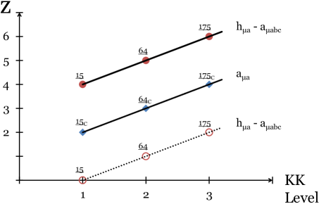
Figure 1: The lower states of the spectrum of Sch${}_{5}(z)$ solutions formed from Kaluza-Klein vector deformations of AdS${}_{5}\times S^{5}$. This is an adaptation of Figure 1 in [33] which depicts the vector mass spectrum, here converted via the massive vector relation $(mL)^{2}_{KK}=z(z+2)$. The $SO(6)$ representation of each vector, listed above each point, partly determines the degeneracy of solutions. At right are the $D=10$ origin of fields, where $\mu$ lies along the noncompact directions and $(a,b,c)$ lie on $S^{5}$. The middle branch of solutions, formed from diagonal vectors descending from the complex two-form, also requires nonzero Kaluza-Klein gravitons not pictured. The lower branch of mixed vectors, while present in the spectrum, gives solutions with negative values of $z$; hence, it appears dotted and unfilled. For details, see the main text.

Generalization to all AdS vacua

The structure of the field equations (2.7), and our analysis thereof, applies equally to the M2-brane solutions constructed in [20]. One might ask whether there is anything special about these two sets of solutions, with an eye toward generalizing this structure to solutions built around any AdS$\times\mathcal{M}$ vacuum.

First, as we will soon note, the fact that the vectors couple quadratically to the gravitons is a completely general phenomenon that derives solely from the Lorentz symmetry of AdS. Combined with the Kaluza-Klein perspective above, it is clear that one can generalize this construction to null deformations of all AdS spacetimes. On the other hand, notice that the mixed vectors do not couple to the gravitons: that is, one might have expected a quadratic source term in $\beta$ to appear in the third (Einstein) equation in (2.7). This absence is likely due to the supersymmetry of the associated AdS solutions, and we remark on this further in section 3.

Summarizing, to each KK vector of an AdS${}_{d+1}\times\mathcal{M}$ compactification, one can associate a set of reduced field equations analogous to (2.7) with at most quadratic source terms. The dynamical exponent $z$ is given precisely by the relation for an effective $d$-dimensional massive vector model,

$$(mL)^{2}_{KK}=z(z+d-2)$$ (2.15)

where the mass is simply the AdS mass of the KK vector: by construction, the same differential operator of $\mathcal{M}$ that gives the spectrum of vector masses is that which gives $z$. If these equations can be solved, one has a solution with Sch${}_{d+1}(z)$ symmetry where the Schrödinger vector is identified with the linearized KK fluctuation. The metric deformation is induced by a tower of massive spin-2 fields that together solve an inhomogeneous Laplace equation with a quadratic source in the vector harmonic.

One can also utilize the spin-2 fields alone to obtain a Schrödinger-symmetric solution, where $z$ is determined by the effective mass of the spin-2 field as

$$(mL)^{2}_{KK}=\left[d+2(z-1)\right]2(z-1)$$ (2.16)

(We will justify this relation for all $d$ later in this section.) Finally, in all of these constructions, the degeneracy of Schrödinger solutions is given by the degeneracy of $\mathcal{M}$ harmonics utilized in the solution.

Analysis of the KK spectrum is based on solving linearized field equations, while the Schrödinger solutions represent solutions of the fully nonlinear theory. In these terms, an obvious question is: how does a solution at linearized level become elevated to a full, nonlinear solution? We now explain how this occurs, first from the point of view of the bulk field equations, and subsequently from the point of view of the holographically dual boundary theory.

2.2 In the bulk: AdS perturbation theory

The message of the above remarks is that one should think of the nonlinear solution as a quadratic extension of a linearized solution around AdS${}_{5}\times SE_{5}$. Thus, our task is to explain why this perturbation theory truncates at second order, and to generalize this fact.

Still referring to the D3-brane case, our strategy will be to initiate a perturbation theory around the AdS solution by seeding it with a linearized vector fluctuation, where the three-form flux has a leg in the $x^{+}$ direction. The fluctuation has some definite weight under the symmetry transformations of the background. Going to higher order in the perturbation theory, the symmetries of this first order solution must be preserved at each order. Furthermore, the possible terms that can get generated must be covariant with respect to the symmetries of the background. In general, this perturbation series will not truncate at finite order; in particular, if one can combine positive powers of the first-order perturbations to form a singlet under all background symmetries, then one will expect this singlet to appear in equations at arbitrary order. Simplification occurs if, for any one symmetry of the background, there are no singlets.

In the case at hand, the Lorentz symmetry of AdS, acting in these coordinates as

$$x^{+}\rightarrow{x^{+}}^{\prime}={x^{+}\over\kappa}\,,\quad x^{-}\rightarrow{x^{-}}^{\prime}=\kappa x^{-}$$ (2.17)

strongly constrains the possible terms that can be generated beyond linear order. Because we seed the perturbation theory with a field with a leg along the null $x^{+}$ direction, and with no legs along the $x^{-}$ direction, this field has weight one under the Lorentz boost. That means that at $n^{th}$ order, the only possible terms that can be generated are of weight $n$. But because the lone symmetric tensor field in our theory is the metric, which has two indices, this perturbation theory will necessarily truncate at quadratic order: there are no possible terms one can write down which turn on a field with Lorentz weight three.

Demonstrating explicitly with the $W\neq 0$ solution based on diagonal vectors, we seed the perturbation via the complex three-form flux, as

$$\begin{split}ds^{2}&=r^{2}\left(2dx^{+}dx^{-}+d\textbf{x}^{2}\right)+\frac{dr^{2}}{r^{2}}+ds^{2}(SE_{5})\\ F_{5}&=4r^{3}dx^{+}\wedge dx^{-}\wedge d\textbf{x}\wedge dr+4Vol_{5}\\ G_{3}&=\delta G_{3}^{(1)}\\ \end{split}$$ (2.18)

with

$$\delta G_{3}^{(1)}=dx^{+}\wedge W$$ (2.19)

We assign $W$ weight one under a Lorentz boost. The only term that can be generated at subsequent orders is the Schrödinger term in the metric,

$$\delta g_{AB}^{(2)}=g_{++}\delta_{A+}\delta_{B+}$$ (2.20)

This fact ensures that the $\partial_{-}$ Killing vector stays null at all orders. Note that we have merely used the Lorentz symmetry of AdS, so this same logic applies to null perturbations of any Lorentz-invariant background by a massive supergravity field. In particular, this argument makes no use of supersymmetry or scale invariance of the near-horizon limit. Note also that the resulting Schrödinger solutions will be at zero temperature, and of the same curvature scale as their AdS counterparts: $L_{Sch}=L_{AdS}$.

This procedure can also be carried out by seeding the perturbation with the mixed KK vectors ($C$), or with the massive spin-2 field ($h$). These first-order choices just preserve different symmetries. In the former case, identical arguments to the above truncate the perturbation theory at second order; in the latter case, since our initial perturbation is of weight two, the linearized solution is in fact a full solution.

In fact, in this example the truncation of perturbation theory works even better than one might have expected. As noted earlier, in the final equation in (2.2) it would be consistent with the Lorentz symmetry to have a $|dC|^{2}$ term appear alongside $|W|^{2}$, but the coefficient of this term is apparently zero. This may be a consequence of supersymmetry, and as we will see, has implications for the robustness of the $C\neq 0$ solutions against higher derivative corrections.

To actually obtain the Schrödinger metric, we turn now to the dilatation symmetry. The full nonlinear solution at hand is not Lorentz invariant, so it is consistent to allow for anisotropic scale invariance (2.5). This fixes the fields $W$ and $g_{++}$ to take their canonical Schrödinger scaling, and enforcement of the Bianchi identity on the three-form flux implies its closure. Parameterizing the metric as $g_{++}=r^{2}h$ gives

$$\begin{split}W&=d(r^{z}\sigma)\\ h&=r^{2z-2}q\\ \end{split}$$ (2.21)

as in (2.4). Both $h$ and $W$ can have functional dependence only on $CY_{3}$ coordinates $(r,\Omega_{5})$: specifically, $x^{-}$ is ruled out because of the $x^{\pm}$ scaling argument, and x is ruled out to preserve rotational symmetry along the brane.

Using the dilatation invariance, general covariance, and the fact that $z=1$ must be an AdS solution for which we can set $W=0$, one can essentially reproduce the reduced field equations (2.7), including the $z$-dependence. Focusing on the spin-2 equation, we know that a two-derivative operator, covariant with respect to the $CY_{3}$ on which the fields are defined, must act on $h$. Scale invariance determines the form of the equation as

$$\nabla^{2}_{CY_{3}}(r^{x}h)=\alpha r^{x}|W|_{10}^{2}$$ (2.22)

for some constants $x,\alpha$, and where the square of $W$ is taken with respect to the 10-dimensional metric. Each side has Lorentz weight two. Substituting from (2.21) gives

$$\left(\nabla^{2}_{5}+(2z+x-2)(2z+x+2)\right)q=\alpha\left(z^{2}|\sigma|^{2}_{5}+|d\sigma|^{2}_{5}\right)$$ (2.23)

We impose one final constraint, which is that when $z=1$, AdS is a solution with $\sigma=0$ and $q$ constant. This determines $x$ as

$$x(x+4)=0$$ (2.24)

The choice $x=0,\alpha=-1$ is evidently made by plugging the ansatz into the Einstein equation itself. Up to this ambiguity, we have thus determined the relation between $z$ and the spin-2 mass, which was unknown a priori, in contrast to the spectrum of $z$ in the well-studied massive vector model.

Thus, it is clear why the field equations (2.7) for the $\sigma=0$ solutions are simply those of the linearized level, and why the $\sigma\neq 0$ solutions have only a quadratic correction to those equations appearing in the Einstein equation. By using the spacetime symmetries of the AdS vacuum we have essentially reproduced all aspects of the nonlinear solution in this perturbative context; we will see in the next section that we can also use the supersymmetry of an AdS solution to make stronger statements about the existence of its Schrödinger deformations away from the supergravity approximation.

First, let us explain the existence of these Schrödinger fixed points from the CFT side.

2.3 On the boundary: conformal perturbation theory

Given the AdS/CFT correspondence, and its generalizations, it is instructive to give a version of our arguments that applies to the boundary theory. As we will see, this corresponds to a simple exercise in conformal perturbation theory. The response of a CFT to a null vector perturbation was studied (along with other aspects of holography for Schrödinger spacetimes) in [26, 27], and we briefly compare our conclusions at the end of this section.

Writing the CFT coordinates as $(x^{\pm},\textbf{x})$, where $x^{\pm}$ are lightcone coordinates, the generators corresponding to dilatations and Lorentz boosts in $x^{\pm}$ act as

$$\begin{split}{\cal D}:\quad&x^{+}\rightarrow{x^{+}}^{\prime}={x^{+}\over\lambda}\,,\quad x^{-}\rightarrow{x^{-}}^{\prime}={x^{-}\over\lambda}\,,\quad\textbf{x}\rightarrow\textbf{x}^{\prime}={\textbf{x}\over\lambda}\\ {\cal L}:\quad&x^{+}\rightarrow{x^{+}}^{\prime}={x^{+}\over\kappa}\,,\quad x^{-}\rightarrow{x^{-}}^{\prime}=\kappa x^{-}\,,\quad\textbf{x}\rightarrow\textbf{x}^{\prime}={\textbf{x}}\end{split}$$ (2.25)

Now consider an operator ${\cal O}_{-}$, whose dilatation weight is $\Delta$, and whose behavior under Lorentz transformation is as indicated by its index structure. Under a combined dilatation and Lorentz transformation it transforms as

$${\cal O}_{-}(x^{+},x^{-},\textbf{x})\rightarrow{\cal O}_{-}({x^{+}}^{\prime},{x^{-}}^{\prime},\textbf{x}^{\prime})=\kappa^{-1}\lambda^{\Delta}{\cal O}_{-}(x^{+},x^{-},\textbf{x})$$ (2.26)

Adding this operator to the Lagrangian obviously breaks Lorentz invariance, and it also breaks scale invariance if $\Delta\neq d$. However, if we write $\Delta$ in the form

$$\Delta=d+z-1$$ (2.27)

we see that under the non-relativistic dilatation generator, ${\cal D}_{z}$, defined as

$${\cal D}_{z}={\cal D}+(z-1){\cal L}$$ (2.28)

and which acts as

$$\begin{split}{\cal D}_{z}:\quad&x^{+}\rightarrow{x^{+}}^{\prime}={x^{+}\over\lambda^{z}}\,,\quad x^{-}\rightarrow{x^{-}}^{\prime}={x^{-}\over\lambda^{2-z}}\,,\quad\textbf{x}\rightarrow\textbf{x}^{\prime}={\textbf{x}\over\lambda}\end{split}$$ (2.29)

the operator ${\cal O}_{-}$ acquires weight $\Delta_{z}=d$ under ${\cal D}_{z}$, and so $\int\!dx^{+}dx^{-}d^{d-2}\textbf{x}{\cal O}_{-}$ is scale invariant, as noted in [26, 27].

Similarly, a spin-2 operator ${\cal O}_{--}$ will be marginal under ${\cal D}_{z}$ provided that its relativistic conformal dimension is $\Delta=d+2(z-1)$.

Perturbing the action as

$$S\rightarrow S+g_{+}\int\!dx^{+}dx^{-}d^{d-2}\textbf{x}~{}{\cal O}_{-}+g_{++}\int\!dx^{+}dx^{-}d^{d-2}\textbf{x}~{}{\cal O}_{--}$$ (2.30)

thus preserves, to first order in the couplings $(g_{+},g_{++})$, scale invariance generated by ${\cal D}_{z}$.

In parallel to our discussion on the gravity side, we can consider the couplings $(g_{+},g_{++})$ as “seeds”, and study the renormalization group beyond first order to see whether scale invariance survives. We proceed using conformal perturbation theory (see [34], section 15.8). Inside the path integral we expand $e^{-S}$ as a power series in the couplings. Ultraviolet divergences can occur when two or more operator insertions coincide in position space, and we regulate these by cutting out a small ball of radius $\Lambda^{-1}$ around each operator, and adding counterterms to remove the divergences. A breakdown of scale invariance is then signalled by the appearance of $\log\Lambda$ terms, since their removal introduces a scale $\mu$.

At second order in perturbation theory a log divergence can occur when two operators collide and produce a factor of $\int{dx^{+}dx^{-}d^{d-2}\textbf{x}\over x^{+}x^{-}|\textbf{x}|^{d-2}}$. In particular, this will happen when the OPE of two vector operators behaves as

$${\cal O}_{-}(x^{+},x^{-},\textbf{x}){\cal O}_{-}(0,0,{\bf 0})\sim{C\over x^{+}x^{-}|\textbf{x}|^{d-2}}{\cal O}_{--}(0,0,{\bf 0})+\cdots$$ (2.31)

where ${\cal O}_{--}$ is a marginal (with respect to ${\cal D}_{z}$) spin-2 operator. In order to renormalize the theory we need to add to the action the operator ${\cal O}_{--}$ with a coefficient that depends logarithmically on scale. The resulting theory thus breaks scale invariance at second order in $g_{+}$ unless $C=0$, with a nonzero $\beta$-function $\beta_{++}\sim C(g_{+})^{2}$.

This behavior corresponds to what we see on the gravity side. Consider an AdS vacuum whose field content includes a massive vector and a massive spin-2 field, whose masses are such that each admits a linearized solution preserving invariance under scale transformation with exponent $z$. In particular, consider the system of equations (2.2), where we assume that the appropriate CY₃ harmonics exist. Now seed a solution with the massive vector $W$. According to the last equation in (2.2) this will source $h$ at quadratic order in $W$. By assumption, at linear order $h$ admits a solution $h\sim r^{2z-2}$, in order to be compatible with the non-relativistic scale invariance. However, at quadratic order in $W$ we will have to shift the power law of $h$ in order to solve the field equations. Expanding in $W$, this gives rise to a term $h\sim|W|^{2}r^{2z-2}\ln r$, whose presence is the bulk analog of the logarithmically running coupling in the CFT. Scale invariance survives only if the source for the marginal $h$ mode vanishes, which is the bulk analog of the CFT condition $C=0$.

In the CFT, checking scale invariance at orders $g_{+}g_{++}$ and $g_{++}^{2}$ means looking for marginal spin-3 and spin-4 operators appearing in the OPEs ${\cal O}_{-}{\cal O}_{--}$ and ${\cal O}_{--}{\cal O}_{--}$. Nonzero OPE coefficients lead to nonzero $\beta$-functions for the spin-3 and spin-4 couplings. Going beyond second order in perturbation theory, we will similarly need to check for the appearance of operators of ever higher spin in OPEs. How do we deal with this? Here the key point is that in the supergravity limit the bulk theory contains no fields of spin larger than two. Such modes would correspond to stringy excitations, which we can think of as having been integrated out, yielding $\alpha^{\prime}$ corrections in the supergravity action. Similarly, in order for the CFT to have a dual supergravity description it is necessary that all single trace operators of higher spin should acquire scaling dimensions that are parametrically large in the large $(\lambda,N)$ limit. So for such CFTs, there will not exist any single trace marginal operators beyond spin-2. Therefore, the full set of renormalization group equations governing the flows seeded by $(g_{+},g_{++})$ consists of the equations $\beta_{+}=0$, $\beta_{++}\sim C(g_{+})^{2}$. Existence of the fixed point thus boils down to checking the single condition $C=0$. As noted above, this matches the behavior seen in the bulk.

The vanishing of $C$ will follow from symmetry in some theories. Namely, if the theory has a global symmetry group under which the marginal spin-1 and spin-2 operators transform, $C$ will vanish unless the product of two spin-1 representations contains the spin-2 representation. For example, in the case of ${\cal N}=4$ SYM, operators will transform in representations of the $SU(4)$ R-symmetry. The same considerations apply on the gravity side, where for example in (2.7) the source terms appearing on the right hand side are subject to the rules governing products of harmonics. (As noted earlier, when $SE_{5}=S^{5}$, $C$ vanishes for all $z$.)

In the bulk, solving the last equation in (2.2) will involve turning on a tower of massive spin-2 two modes with amplitudes proportional to the square of the vector field. We can make a parallel observation on the CFT side. Let us consider a tower of generically non-marginal spin-2 operators ${\cal O}_{--}^{(n)}$. In order to talk about the flow of their couplings $g^{(n)}_{++}$, let us now work in terms of the Wilsonian renormalization group, where we keep track of all couplings, not just the marginal and relevant ones. Lorentz invariance now constrains their $\beta$-functions to be of the form

$$\begin{split}\beta_{++}^{(n)}&=\left(\Delta_{z}[{\cal O}_{--}^{(n)}]-d\right)g_{++}^{(n)}+C^{(n)}(g_{+})^{2}\end{split}$$ (2.32)

where $\Delta_{z}[{\cal O}_{--}^{(n)}]$ are the operator dimensions at the Lorentz invariant fixed point. We are including only the effect of couplings with purely $+$-type indices, since all other couplings can be consistently set to zero by Lorentz invariance. Along with the fact that the equation $\beta_{+}=0$ is uncorrected by the presence of $g_{++}^{(n)}$, which again follows from Lorentz invariance, we find the fixed point by taking

$$g_{++}^{(n)}=-{C^{(n)}\over\Delta_{z}[{\cal O}_{--}^{(n)}]-d}(g_{+})^{2}$$ (2.33)

We can now see the parallel with the gravity side. According to (2.7), scale invariant solutions are found by solving an inhomogeneous Laplace equation for $q$, with the source given by the square of the vector field. The solution can be decomposed into the harmonics for the massive spin-2 fields. The solution will then contain a tower of massive spin-2 fields with amplitudes proportional to the square of the vector, which is what we have in (2.33). To make this connection precise we would like a better understanding of the bulk interpretation of the Wilsonian couplings; see [37, 38] for recent work in this direction.

Finally, let us remark on references [26, 27], which argued that couplings for vector operators ${\cal O}_{-}$ are exactly marginal with respect to non-relativistic scale transformations. The arguments in [26, 27] were based on showing that the 2-point function for ${\cal O}_{-}$ is uncorrected by the addition of ${\cal O}_{-}$ to the Lagrangian. This establishes that $\beta_{+}=0$; however one also needs to verify that $\beta$-functions for other couplings vanish as well. As we discussed above, this corresponds to checking that no marginal spin-2 operators appear in the OPE of the vector operators, and this has a direct correspondence with the field equations in the bulk.

2.4 A corollary: consistent truncations with massive KK modes

Before moving on, we can apply our conclusion to the construction of consistent truncations of string/M-theory. By now, there is a large amount of technology for constructing consistent truncations with massive modes, e.g. [10, 11, 12, 13, 14, 15, 16, 17, 39], and it was in this manner that the first string/M-theory embeddings of Schrödinger solutions were found in [10]. We have shown here that one can always elevate the linearized vector and spin-2 fluctuations around AdS to part of a full, nonlinear Schrödinger solution; but if one can elevate some of these fields to the nonlinear level on the level of the action itself, then it is clear that Schrödinger solutions to such theories always exist.

Therefore, a corollary to our argument is that anytime there exists a consistent truncation of an AdS$\,\times\,\mathcal{M}$ KK spectrum that includes massive vector and/or spin-2 fields, the truncated theory admits the associated Schrödinger solutions.

When can this be done? Although some recent work [11, 14] has argued for the possibility of including massive spin-2 fields in truncations to maximally supersymmetric supergravities, old lore [40] and new evidence [41] point to the contrary. If it is indeed true that no spin-2 fields can be so included – supersymetrically or otherwise – then the Schrödinger solutions built on diagonal vectors that also turn on a tower of spin-2 fields cannot be found as solutions of consistent truncations. In type IIB solutions, this excludes all but those that can be attained by a TsT transformation.

On the other hand, the solutions built from mixed vectors have no associated spin-2 fields. In principle, all of these solutions are ripe for embedding; in practice, all massive truncations to date have only included vector harmonics that sit at the base of their respective KK towers.

It was conjectured in [13] that a necessary condition for the consistency of the inclusion of a massive KK mode is that the field sits at the bottom of its tower, based on consideration of structure groups of compactification manifolds. If we take this to be true as well, then the possibilities for embedding Schrödinger solutions into string/M-theory by fitting them into consistent truncations are severely limited; for example, no more of the D3-deformed Schrödinger solutions can find such an embedding.

The flipside of this would be the implication that anytime a massive vector is included in a consistent truncation, it can be used to construct a Schrödinger solution. This would provide a trivial prescription for identifying non-relativistic vacua, and at least gives a rule of thumb. We give an example later on of a supersymmetric truncation to a $d=4$, $\mathcal{N}=2$ gauged supergravity arising from wrapped M5 branes that includes a massive vector multiplet [42], and show that, indeed, two Schrödinger solutions exist in correspondence to the theory’s two AdS₄ vacua.

3 Quantum/string corrections

We turn now to the study of corrections to Schrödinger solutions due to quantum and string effects, which hinges on analyzing corrected KK spectra of AdS vacua. In what follows, there is no distinction made between $\alpha^{\prime}$ corrections and $G_{N}$ corrections, as both enter on equal footing as higher derivative terms. For convenience we sometimes refer to these collectively as $\alpha^{\prime}$ corrections.

Let us first ask whether the existence of a solution is affected by $\alpha^{\prime}$ corrections.

For Schrödinger solutions built on KK vectors and gravitons that do not couple to each other – these are the $q\neq 0$ and $\beta\neq 0$ solutions of section 2.1, for example – we can quickly establish that there will always exist Schrödinger solutions at every order in a higher derivative expansion. Assuming that the curvature does not become so large as to invalidate the gravity description, then there will always exist Schrödinger solutions made by utilizing the KK spectrum around the new, corrected vacuum in the preceding manner. This will generically induce a shift in $z$ and $L_{Sch}$, and is a generalization of a statement made in [28]. Using the dual arguments on the CFT side made in the previous section, the lone effect of heavy operators is to rescale dimensions such that a given operator is now marginal with respect to the new, shifted non-relativistic dilatations.

On the other hand, for Schrödinger solutions built on KK modes that do couple, i.e. when the graviton mode obeys an inhomogeneous Laplace equation – these are the $q,\sigma\neq 0$ solutions of section 2.1, for example – there may not be a solution upon including $\alpha^{\prime}$ corrections. $z$ is determined by the vector spectrum, which will be shifted by the correction terms, and this induces a change in the quadratic source term: consequently, the corrected Einstein equation may not be soluble for a fixed vector harmonic. On the CFT side, the statement is that with respect to the new non-relativistic dilatations, there may exist a marginal spin-2 operator that appears in the OPE of two marginal vectors. In other words, the first term in (2.32) may vanish, eliminating the fixed point.

What is required of the AdS background for these corrections to vanish? As one might expect, the answer is supersymmetry. And as we show momentarily, certain families of Schrödinger solutions built from perturbations of the maximally supersymmetry AdS spacetimes are exact.

The outline for this section is as follows. In 3.1, we utilize supersymmetry in presenting the conditions for nonrenormalization, and the aforementioned exact solutions. In 3.2, we explicitly show how one class of exact solutions with Sch₅ symmetry, obtained by deformation of AdS${}_{5}\times S^{5}$, remains a solution to $O(\alpha^{\prime 3})$ despite its reduced isometry and supersymmetry. This is done by direct calculation with the conjectured metric and five-form flux correction terms at this order in the type IIB supergravity action.

3.1 Uncorrected Schrödinger solutions from short multiplets

In the presence of supersymmetry, there will typically be some degree of nonrenormalization of the AdS background and its KK spectrum. In cases for which the AdS background itself is robust against renormalization to some order in a derivative expansion, Schrödinger solutions built from perturbations of this background are similarly robust, as $L_{AdS}=L_{Sch}$.

The most useful fact for our purposes is basic: if a supergravity mode lies in a shortened multiplet of the corresponding AdS supergroup, then the exponent appearing in a power law profile for such a mode cannot get renormalized at any order in higher derivative corrections. This can be understood intuitively as follows. The action of the dilatation operator directly relates the exponent to the scaling dimension of the dual boundary CFT operator; but operators in short multiplets have protected scaling dimensions. Since $z$ appears as such an exponent, it will hence not be renormalized. Shortened multiplets occur, for instance, for all supergravity modes in maximally symmetric spacetimes because a long multiplet necessarily has fields with spins greater than two. Such shortened multiplets are actually ubiquitous in KK spectra, as many supergroups without maximal symmetry possess some number of short multiplets.

This immediately implies that if an AdS supergroup admits shortened multiplets, the Schrödinger solutions built from the massive fields in those multiplets will receive some level of protection from renormalization to all orders. Specifically, any property of the solution that depends only on the mass of such a field will be unrenormalized. Of course, this is the case for the dynamical exponent $z$ which is determined by either a vector or spin-2 equation; see (2.7). Therefore, we conclude that if the KK field that determines $z$ sits in a short multiplet, $z$ will remain uncorrected to all orders in an $\alpha^{\prime}$ expansion.

The reason that all solutions are not fully protected is that the perturbation theory around AdS truncates at quadratic, not linear, order. In our canonical D3 brane example of section 2.1, those solutions formed from a diagonal vector ($\sigma\neq 0$) obey a spin-2 field equation corrected by a quadratic term. Thus, even if the spin-2 field $h$ is in a short multiplet, the solution will receive a correction. On the other hand, the solutions built on linear Laplace equations receive no renormalization at all, because all properties of the solution are derived from field equations which remain uncorrected in the full solution.

We summarize these results as follows:

Suppose we have an AdS$\times\mathcal{M}$ solution which remains unrenormalized to $n^{th}$ order in $\alpha^{\prime}$ or $l_{P}$. This implies that $L_{Sch}$ will follow suit. We now ask what other renormalization can occur. Suppose the KK spectrum contains both vectors and gravitons in short multiplets, and we turn these fields on to generate a Schrödinger geometry. The following nonrenormalization theorems will hold:

• Vector and graviton do not couple: The reduced field equations are simply those of the linearized fluctuations. So the full solution, modulo $L_{Sch}$, remains unrenormalized to all orders in higher derivative corrections.

• Vector and graviton couple: This requires a tower of nonzero gravitons as well, which collectively solve a Laplace equation with a quadratic source. This solution will have $z$ unrenormalized, but the functional dependence of $g_{++}$ on $\mathcal{M}$ coordinates will be corrected at higher orders. (Again, $L_{Sch}$ is unchanged to $n^{th}$ order only.)

All of these arguments can be straightforwardly made on the CFT side, in accordance with the discussion in subsection 2.3.

In application to our D3-brane example of section 2, note that the uncoupled solutions (mixed vector and spin-2) are supersymmetric, generically preserving one half of the Poincaré supersymmetries of the AdS background [18, 19]. The coupled solutions (diagonal vector) can be made supersymmetric, but need not be [20, 21, 22].

3.1.1 Exact solutions

When the AdS spacetime around which we perturb is maximally supersymmetric, $L_{AdS}=L_{Sch}$ receives no rescaling to all orders in higher-derivative corrections [43], and all supergravity fields belong to short multiplets. Such spacetimes are the near-horizon geometries of the conformal branes in type IIB string theory and M-theory. Therefore, the towers of Schrödinger solutions based only on mixed vector and spin-2 perturbations of the maximally supersymmetric AdS${}_{4/5/7}\times S^{7/5/4}$ vacua are exact. These solutions preserve eight Poincaré supercharges [20], and are of course not maximally isometric. As such, we add them to the short list of exact solutions with less than maximal supersymmetry and isometry, including the non-supersymmetric plane wave spacetimes studied in [44] and the 1/4 BPS AdS${}_{2}\times S^{2}$ vacuum of $\mathcal{N}=2,d=4$ supergravity without matter multiplets [43].

On the CFT side, this says that there exist Galilean-invariant vacua for arbitrary ’t Hooft coupling and number of colors. In $\mathcal{N}=4$ SYM, the $(2,0)$ theory on M5 branes and the CFT on M2 branes, the conformal phase can be broken to a Galilean-symmetric phase with $z$ fixed as a function of $\lambda$ or $N$.

When the spheres are replaced by manifolds with less isometry, the resulting AdS vacua will have partial or no supersymmetry. Still, it is known in some cases that $L_{AdS}$ is norenormalized to a certain order in the derivative expansion. For example, using the conjectured $O(\alpha^{\prime 3})$ correction terms of type IIB involving the metric and five-form only [29, 45], it has been shown that the AdS${}_{5}\times SE_{5}$ vacuum is unrenormalized to this order. Thus, the solutions with Sch₅ symmetry built by perturbing this background with massive fields in short multiplets, while keeping $\sigma=0$, are unrenormalized to this order too. The same goes for the AdS${}_{3}\times S^{3}\times M_{4}$ geometry of the strongly coupled D1-D5 system, and its associated Sch₃ solutions which we present in section 4.

Indeed, the $SU(2,2|1)$ supergroup of the AdS${}_{5}\times SE_{5}$ vacuum is one of many that contains short multiplets. The shortening conditions for $SU(2,2|\mathcal{N})$, with $\mathcal{N}=1,2,4$, are summarized in [46]. The most well-studied example of a geometry dual to an $\mathcal{N}=1$ SCFT, AdS${}_{5}\times T^{1,1}$, has both spin-2 and spin-1 fields in semi-long multiplets [47], dual to boundary operators of protected, rational conformal dimension. So solutions based on these fields are unrenormalized to at least $O(\alpha^{\prime 3})$.

Other AdS vacua whose KK spectra contain states in short multiplets include: AdS${}_{3}\times S^{3}$ solutions of various $d=6$ supergravities, the multiplet structure of which was given in [48]; AdS${}_{4}\times SE_{7}$ solutions, the supergravity states of which fall into unitary irreducible representations of $OSp(2|4)$ (e.g. [49, 50]); and orbifolded AdS vacua.

3.2 At $O(\alpha^{\prime 3})$, explicit nonrenormalization of Sch₅

We focus on type IIB Sch₅ solutions because, relatively speaking, we know a lot about type IIB correction terms. We possess an explicit form for the terms involving only the metric and five-form up to $O(\alpha^{\prime 3})$ relative to the supergravity action; we know that the supersymmetry of AdS${}_{5}\times SE_{5}$ vacua renders their length scales fixed to this order; and we know that when $SE_{5}=S^{5}$, the solution is maximally symmetric, maximally supersymmetric, and hence unrenormalized to all orders, inclusive of corrections from all type IIB fields.

The full set of metric and five-form corrections at $O(\alpha^{\prime 3})$ was presented in [29], building on the conjecture of [45]. There exists a scheme, obtained by appropriate definition of the metric, in which the metric dependence can be written in terms of only the Weyl tensor, $C_{ABCD}$. All appearance of the five-form flux is via the following two-derivative tensor [51],

$$\mathcal{T}_{ABCDEF}=i\nabla_{A}F_{BCDEF}+\frac{1}{16}(F_{ABCMN}F_{DEF}^{\phantom{DEF}MN}-3F_{ABFMN}F_{DEC}^{\phantom{DEC}MN})$$ (3.1)

where $[A,B,C]$ and $[D,E,F]$ should be independently antisymmetrized, and the two sets symmetrized under interchange. Schematically, the corrections to the Lagrangian take the form

$$C^{4}\,,\quad C^{3}\mathcal{T}\,,\quad C^{2}\mathcal{T}^{2}\,,\quad C\mathcal{T}^{3}\,,\quad\mathcal{T}^{4}$$ (3.2)

along with their complex conjugates, all entering at $O(\alpha^{\prime 3})$; the full set of contractions is determined in [29]. The terms enter the Einstein frame action as [29, 45]

$$S^{(3)}\sim\alpha^{\prime 3}\int d^{10}x\sqrt{-g}f^{(0,0)}(\tau,\bar{\tau})(C^{4}+\ldots)$$ (3.3)

where

$$f^{(0,0)}(\tau,\bar{\tau})=\sum_{(m,n)\neq(0,0)}\frac{\tau_{2}^{3/2}}{|m+n\tau|^{3/2}}$$ (3.4)

is a modular form [52] written in terms of the axio-dilaton $\tau=\tau_{1}+i\tau_{2}=\chi+ie^{-\phi}$, and the well-known $C^{4}$ term [53] is

$$C^{4}=C^{ABCD}C_{EBCF}C_{A}^{\phantom{A}GHE}C^{F}_{\phantom{F}GHD}+\frac{1}{2}C^{ABCD}C_{EFCD}C_{A}^{\phantom{A}GHE}C^{F}_{\phantom{F}GHB}$$ (3.5)

Beyond this order in $\alpha^{\prime}$, the structure of the corrections is not known.

For the AdS${}_{5}\times S^{5}$ background, in which $L_{AdS_{5}}=L_{S^{5}}$, superspace arguments have been used to prove that the solution is exact [43] . This is clearly satisfied at $O(\alpha^{\prime 3})$, as one can show that $C=\mathcal{T}=0$ on this solution. The uncorrected KK spectrum of energies is also evidently unrenormalized at this order: the corrections are quartic in $C$ and $\mathcal{T}$, so variation will never give a term linear in only one of these tensors.

Using this apparatus, we now consider corrections to the Sch₅ solutions obtained by deformations of AdS${}_{5}\times S^{5}$. We will explicitly demonstrate what we argued for earlier: that the metric and five-form solutions ($\sigma=0$) are unrenormalized, but that those with three-form flux ($\sigma\neq 0$) can receive a renormalization of the $S^{5}$ part of $g_{++}$. We consider these in turn, keeping $\beta=0$ for simplicity.

Before we begin, let us give away the punchline. It may seem like something of a mystery that these Sch₅ geometries, despite their greatly reduced supersymmetry and isometry, are as robust against these same corrections as the maximally supersymmetric and isometric AdS${}_{5}\times S^{5}$. As with many other aspects of Schrödinger holography, the null Killing vector is the key.

3.2.1 Sch₅ solutions from AdS${}_{5}\times S^{5}$: $\sigma=0$

This solution has metric and five-form flux only, so the only terms that can contribute to renormalization are the terms given above, plus terms linear in the axio-dilaton and complex three-form flux which can turn on a decoupled field. We delay treatment of these latter terms temporarily, as we turn to the $O(\alpha^{\prime 3})$ metric and five-form terms.

Our strategy will be to look for terms which contribute to $C$ and $\mathcal{T}$ – each of which vanishes in AdS₅ – and show that there are not enough terms to give nonzero contractions when plugged into the correction terms from (3.2).

The Sch₅ metric

$$ds^{2}=r^{2z}q(dx^{+})^{2}+ds^{2}(AdS_{5}\times S^{5})$$ (3.6)

corrects the vanishing AdS${}_{5}\times S^{5}$ Weyl tensor only by terms which have two lower + indices and no - indices. Specificially, nonvanishing components are

$$C_{+r+\theta_{i}}\,;\quad C_{+\theta_{i}+\theta_{j}}\,;\quad C_{+r+r}\,;\quad C_{+\textbf{x}+\textbf{x}}$$ (3.7)

where $\{\theta_{i}\}$ parameterize $S^{5}$. There are no lower - indices. Already, this implies that variation of the $C^{4}$ term will vanish on-shell, because the + indices have nothing to contract with: $g^{++}=0$.

The correction terms are quadratic in $C$ and $\mathcal{T}$, so variation of these terms with respect to either $F_{5}$ or the metric will leave behind terms at least cubic in $C$ and $\mathcal{T}$. Because $g^{++}=0$, this implies that if $\mathcal{T}$ has no components with lower - indices, all variation of the correction terms will vanish: the lower + indices of either tensor will not have any upper + indices to contract with, and the quartic order guarantees enough index contractions to force such a contraction. So, we examine the structure of $\mathcal{T}$, given in (3.1).

Recall that $\mathcal{T}=0$ in AdS${}_{5}\times S^{5}$. We can uncover the structure of this term in the Schrödinger vacuum without actually plugging in for the flux – which is the same in both Schrödinger and AdS backgrounds, namely the sum of volume forms – by asking what new components of the Christoffel connection and contravariant metric are introduced by the deformation.

The new components of the connection are

$$\begin{split}&\Gamma^{r}_{++}=-qzr^{2z+1}\,,\quad\Gamma^{-}_{+r}=qr^{2z-3}(z-1)\,,\\ &\Gamma^{-}_{+\theta_{i}}=\frac{1}{2}r^{2z-2}\frac{\partial q}{\partial{\theta_{i}}}\,,\quad\Gamma^{\theta_{i}}_{++}=-\frac{1}{2}r^{2z}\frac{\partial q}{\partial{\theta_{i}}}\\ \end{split}$$ (3.8)

This implies that the flux remains covariantly constant in the Schrödinger background,

$$\nabla_{A}F_{BCDEF}=0$$ (3.9)

This relies on the fact that the flux is merely the sum of the two volume forms, just as in AdS${}_{5}\times S^{5}$, and the fact that none of the new Christoffel components has an identical upper and lower index.

Now we examine the terms quadratic in $F_{5}$. Because the components of $F_{5}$ are the same as in AdS₅, the only changes will come from new contravariant components of the metric, of which there is one: $g^{--}\neq 0$. This implies the existence of a single new nonzero term. Consider the contraction

$$F_{ABC-G}F_{DEF}^{\phantom{DEF}-G}=F_{ABC-G}F_{DEF+}^{\phantom{DEF+}G}g^{+-}+F_{ABC-G}F_{DEF-}^{\phantom{DEF-}G}g^{--}$$ (3.10)

The second term is the new term; the first term merely contributes to the condition $\mathcal{T}=0$ in the unperturbed AdS background. Looking at the new term, we see that $G\neq+$, otherwise it vanishes. So one index within each triplet $[A,B,C]$ and $[D,E,F]$ must be the + index. Hence, the new term takes the schematic form

$$\mathcal{T}_{+BC+EF}\sim F_{+BC-G}F_{+EF-}^{\phantom{+EF-}G}g^{--}$$ (3.11)

where $B,C,E,F\neq-$. More specifically, the only nonvanishing terms are

$$\mathcal{T}_{+xy+xy}\,,\quad\mathcal{T}_{+rx+rx}\,,\quad\mathcal{T}_{+ry+ry}$$ (3.12)

because $F_{+-rxy}\neq 0$ is the only nonvanishing flux component with legs along $+$.

To summarize, the only nonvanishing components of $\mathcal{T}$ and $C$ have no lower - indices, and hence any variation of the correction terms will vanish on-shell.

This is a perhaps surprising result. To further drive the point home, we point out an argument in [29] that any solution with all fields trivial except for the metric and five-form that is more than 1/4 BPS is uncorrected at $O(\alpha^{\prime 3})$ by the entire set of terms above. Here, we have shown the same for these 1/4 BPS solutions.

We now turn to possible terms linear in the axio-dilaton and three-form flux, which would act as sources for these fields. Symmetry under $G_{3}\rightarrow-G_{3}$ rules out terms linear in $G_{3}$. Terms linear in the axio-dilaton would, at this order, be multiplied against a scalar, eight-derivative object constructed from the Weyl tensor and five-form field strength. Further, any such scalars must vanish when evaluated on the AdS background, since this is a solution by assumption. Schematically, this would allow terms such as

$$(\phi,\chi)\,C_{ABCD}\left((F_{5})^{6}\right)^{ABCD}\,,\quad(\phi,\chi)\,\nabla_{A}C_{BCDE}\left((F_{5})^{5}\right)^{ABCDE}\,\ldots$$ (3.13)

However, by examining the index structure and using the null Killing vector, one can check that all such scalar terms vanish. We conclude that the axio-dilaton is not sourced at this order.

3.2.2 Sch₅ solutions from AdS${}_{5}\times S^{5}$: $\sigma\neq 0$

Now we turn on three-form flux. This does not affect the metric and five-form correction analysis above. So if this solution is to be renormalized, it must come from the three-form terms. In the absence of knowledge of the actual form of the terms, the null constraint is not strong enough to rule this out.

Let us at least present the challenge. First, $F_{5}$ is not constrained to appear via the $\mathcal{T}$ tensor in these terms. This introduces a tensor component with a lower - index, $F_{+-rxy}$, as well as one without any + or - indices at all, $F_{\theta_{1}\ldots\theta_{5}}$. The metric still must appear via the Weyl tensor, still as in (3.7), so the full set of nonzero components is

$$C_{+A+B}\,,\quad F_{+-rxy}\,,\quad F_{\theta_{1}\ldots\theta_{5}}\,,\quad G_{+r\theta_{i}}\,,\quad G_{+\theta_{i}\theta_{j}}$$ (3.14)

Additionally, $G_{3}$ is not covariantly constant, so we can have $\nabla G_{3}$ appear in the correction terms.

Suppose we wish to ask what terms can contribute to the stress tensor. The following term is explicitly nonvanishing on this background, and could arise at $O(\alpha^{\prime 3})$:

$$\begin{split}(G^{2}F^{6})_{++}&\sim G_{+BC}G_{+DE}F^{BCFGH}F^{DE}_{\phantom{DE}FGH}F^{4}\\ &\sim G_{+\theta_{i}\theta_{j}}G_{+\theta_{k}\theta_{l}}F^{\theta_{i}\theta_{j}\theta_{m}\theta_{n}\theta_{p}}F^{\theta_{k}\theta_{l}}_{\phantom{\theta_{k}\theta_{l}}\theta_{m}\theta_{n}\theta_{p}}F^{4}\end{split}$$ (3.15)

where $F^{4}$ includes all possible contractions. Another term is

$$\begin{split}(G^{2}F^{6})_{++}&\sim F_{+ABCD}F_{+E}^{\phantom{+E}BCD}G^{AGH}G^{E}_{\phantom{E}GH}F^{4}\\ &\sim F_{+-rxy}F_{+-}^{\phantom{+-}rxy}G^{-GH}G^{-}_{\phantom{-}GH}F^{4}\\ \end{split}$$ (3.16)

The correct properties under symmetry are manifest for both of these terms.

Therefore, the null Killing vector does not imply an absence of renormalization of the $g_{++}$ component of these Sch₅ solutions. It is quite possible, if not likely, that the true three-form correction terms involve a tensor structure, analogous to $\mathcal{T}$ for the five-form and metric terms, that renders the corrections to the Sch₅ backgrounds zero.

4 New Schrödinger solutions

We put our theory into practice by presenting new Schrödinger solutions. Two of these are based on the compactification spectra of well-studied brane setups: the maximally supersymmetric M5 brane in flat space, and the half-supersymmetric D1-D5 system of type IIB with the D5 brane wrapped on $T^{4}$ or $K3$. The third construction presents evidence for our earlier suggestion that all consistent truncations of string/M-theory that retain massive modes admit Schrödinger solutions. In this instance, we build a pair of Sch₄ solutions dual to nonrelativistic phases of a 2+1 CFT living on M5 branes wrapped on special-Lagrangian 3-cycles of a Calabi-Yau.

The M5 construction includes two infinite families of solutions exact to all orders in $l_{P}$. The D1-D5 construction includes three families that are exact up to the order at which $L_{AdS_{3}}$ is rescaled.

4.1 Sch₇ from M5 branes

The KK spectrum around AdS${}_{7}\times M_{4}$ [55, 56] contains two towers of mixed vectors, no massive diagonal vectors, and massive gravitons as always. This spacetime has $L_{AdS_{7}}=2L_{M_{4}}\equiv 2$. For $M_{4}=S^{4}$, the upper branch of vectors has masses $m^{2}=(l+3)(l+5)$ (where integer $l\geq 0$ henceforth), implying a (positive) $z$ spectrum of $z=6+2l$, in accordance with (2.15). The massive gravitons have spectrum $m^{2}=(l+1)(l+4)$, which implies a (positive) $z$ spectrum of $z=2+l$, in accordance with (2.16).

If one replaces $S^{4}$ with an $M_{4}$ which has nonzero second Betti number $b_{2}$, there will be an additional set of Yang-Mills gauge fields in $d=7$. These Betti vectors carry topological charge, descending directly from the three-form gauge field and appearing as a single harmonic level of diagonal vectors. Their masslessness gives an isolated Sch₇ solution with $z=-4$ and degeneracy $b_{2}$; the possibility $z=0$ is ruled out, as the Schrödinger vector in this case would be pure gauge.

We will realize each one of these solutions in $D=11$, again starting from the full M5-brane metric and then moving into the near-horizon. The most general solution is

$$\begin{split}ds^{2}&=\Phi^{-1/3}(2dx^{+}dx^{-}+h(dx^{+})^{2}+2dx^{+}C+d\textbf{x}^{2})+\Phi^{2/3}ds^{2}(X_{5})\\ G&=\star_{11}(dx^{+}\wedge dx^{-}\wedge d\textbf{x}\wedge d\Phi^{-1})+dx^{+}\wedge V-\star_{11}(dx^{+}\wedge d\textbf{x}\wedge d(\Phi^{-1}C))\\ \end{split}$$ (4.1)

This ansatz preserves rotational invariance. $C$ is a one-form, $V$ is a three-form, and $h$ is a function, all defined on the space $X_{5}$. The Maxwell and Einstein equations, and the Bianchi identity, imply

$$\begin{split}&d\star_{X_{5}}\Phi=0\\ &d\star_{X_{5}}dC=0\\ &d\star_{X_{5}}\left(\frac{V}{\Phi}\right)=0\\ &dV=0\\ &\nabla^{2}_{X_{5}}h=-\frac{1}{\Phi}|V|^{2}_{X_{5}}\\ \end{split}$$ (4.2)

where $|V|^{2}_{X_{5}}=\frac{1}{3!}V_{abc}V^{abc}$ with indices raised by the metric on $X_{5}$. Notice the extra factors of $\Phi$ in the $V$ terms relative to the D3 brane case (cf. equations (2.2)).

Set $V=0$ for now. Zooming into the near-horizon region and writing $X_{5}$ as a cone over $M_{4}$,

$$ds^{2}(X_{5})=dr^{2}+r^{2}ds^{2}(M_{4})$$ (4.3)

we make the scale-invariant assignments

$$\begin{split}\Phi=r^{-3}\\ C=r^{\frac{z-2}{2}}\beta\\ h=r^{z-1}q\\ \end{split}$$ (4.4)

where $q$ and $\beta$ are a function and one-form, respectively, on $M_{4}$. When $V=0$, this is a solution so long as the reduced field equations

$$\begin{split}&\Delta_{4}\beta=\frac{z(z-2)}{4}\beta\quad\text{where}\quad d\star_{4}\beta=0\\ &\nabla^{2}_{4}q+(z-1)(z+2)q=0\\ \end{split}$$ (4.5)

are satisfied, with $-\nabla^{2}_{4}$ and $\Delta_{4}$ as the Laplace operator of $M_{4}$ acting on functions and transverse one-forms, respectively. For a spherical base space $M_{4}=S^{4}$,

$$\Delta_{4}\beta=(l+2)(l+3)\beta\,,\quad\nabla^{2}_{4}q+l(l+3)q=0$$ (4.6)

and we obtain the anticipated spectra of $z$ outlined earlier. Notice that these two solutions can be consistently superposed, because there exist simultaneous eigenfunctions of $\Delta_{4}$ and $-\nabla^{2}_{4}$ for all $z$.

Because all KK fields sit in short multiplets of the superalgebra $OSp(8|4)$ [56], these solutions are exact. By inspection of the structure of this solution, we expect it to preserve eight Poincaré supersymmetries, in analogy with the M2 and D3 brane solutions of [20].

Turning to $V\neq 0$, the discussion at the start of this subsection implies the existence of a single solution with $z=-4$ corresponding to deformation by the $b_{2}$ topological vector fields. Indeed, one can show that the following configuration solves the field equations,

$$V=d(r^{-2}\tau)$$ (4.7)

where $\tau$ is a harmonic two-form on $M_{4}$, $d\tau=d\star_{M_{4}}\tau=0$. So $M_{4}$ must have $b_{2}\neq 0$, and scale invariance of $G$ implies $z=-4$ as predicted, since $V$ must scale as $r^{z/2}$. The associated Einstein equation is

$$\nabla^{2}_{4}q+10q=-4|\tau|_{4}^{2}$$ (4.8)

Perhaps unexpectedly, this is but one of an infinite family of diagonal solutions, despite the absence of diagonal vectors in the spectrum of KK fields on AdS${}_{7}\times M_{4}$. We present the general construction in appendix A, along with a Lif${}_{6}(z=2)$ solution obtained in a similar manner.

4.2 Sch₃ from D1-D5 and F1-NS5 branes

These solutions come from deformations of AdS${}_{3}\times S^{3}\times M_{4}$, with $M_{4}=T^{4},K3$. The KK spectra [58] around these two solutions are identical in everything but multiplicities of fields, on account of the different number of tensor multiplets in the chiral and non-chiral $d=6$ supergravities. They are somewhat more involved than the examples presented so far because of the prior reduction on $M_{4}$, combined with the self-duality properties of the tensor fields. As a result, we relegate a full treatment to an appendix and only present the solutions here.

Once again, we expect these solutions to have the same supersymmetric structure as their D3 and M2-brane counterparts: the mixed solutions should preserve half of the Poincaré supersymmetry of the D1-D5 background, and the diagonal solutions can, but need not, be supersymmetric. We have not confirmed this explicitly, however.

The KK reduction on $S^{3}$ is done at the level of the $d=6$ supergravity, which contains five self-dual and $n_{T}$ anti-self-dual tensor fields that descend from the complex three-form and five-form fluxes, where $n_{T}$ is the number of antisymmetric tensor multiplets.

4.2.1 Diagonal vectors

There are two towers of diagonal vectors, each with mass $(mL)^{2}=(l+2)^{2}$, implying a $z$ spectrum of $z^{2}=(l+2)^{2}$, where $l\in\mathbb{Z}$. One tower descends from the four self-dual tensor fields that do not source the D1-D5 background, and the other from the $n_{T}$ anti-self-dual tensor fields.

The ansatz is

$$\begin{split}&ds^{2}=r^{2z}q(dx^{+})^{2}+2r^{2}dx^{+}dx^{-}+\frac{dr^{2}}{r^{2}}+ds^{2}(S^{3})+ds^{2}(M_{4})\\ &iG_{3}=2(1+\star_{6})d\Omega_{3}+\delta F_{3}-i\delta H_{3}\\ &F_{5}=\delta F_{5}\\ \end{split}$$ (4.9)

where $q$ is a function defined on $S^{3}$, $d\Omega_{3}$ is the invariant volume form on $S^{3}$, and $\star_{6}$ is the Hodge star operator on the spacetime transverse to the $M_{4}$. We have set $L_{AdS_{3}}=L_{S^{3}}=1$. When $q=\delta H_{3}=\delta F_{3}=\delta F_{5}=0$, this is the D1-D5 solution.

Because the $d=6$ tensor fields descend from both $G_{3}$ and $F_{5}$, we simply need to turn on the components of $G_{3}$ and $F_{5}$ that give rise to tensor fields with the right $d=6$ self-duality property. This means that we can turn on anti-self dual parts of $F_{3},H_{3}$ and $F_{5}$, but only self-dual parts of $H_{3}$ and $F_{5}$. This also implies that without doing any extra work, the F1-NS5 system obtained from the D1-D5 system by S-duality can also be engineered to give Schrödinger solutions in exactly the same way: from the six-dimensional perspective, S-duality merely shuffles the background flux to a different one of the five self-dual tensor fields.

Without further ado, the solutions are:

• Anti-self-dual RR two-form charge:

  $$\delta F_{3}=(1-\star_{6})dx^{+}\wedge d(r^{z}\sigma)$$ (4.10)

• NS-NS two-form charge:

  $$\delta H_{3}=(1\pm\star_{6})dx^{+}\wedge d(r^{z}\sigma)$$ (4.11)

• RR four-form charge:

  $$\delta F_{5}=\frac{1+\star_{10}}{\sqrt{2}}\left[(1\pm\star_{6})dx^{+}\wedge d(r^{z}\sigma)\wedge\alpha\right]$$ (4.12)

$\sigma$ is a one-form on $S^{3}$, $\alpha$ is a harmonic two-form on $M_{4}$ of norm $|\alpha|^{2}=1$ and definite $M_{4}$ self-duality property, and the reduced field equations are

$$\begin{split}&\Delta_{3}\sigma=z^{2}\sigma\quad\text{where}\quad d\star_{3}\sigma=0\\ &\nabla^{2}_{3}q+4z(z-1)q=-2\left(z^{2}|\sigma|_{3}^{2}+|d\sigma|_{3}^{2}\right)\\ \end{split}$$ (4.13)

with $-\nabla^{2}_{3}$ and $\Delta_{3}$ as the Laplace operator of $S^{3}$ acting on functions and transverse one-forms, respectively. Note that the source terms in the Einstein equation are of the same form as those in the D3-brane case, given in (2.7). For future reference, let us denote this quantity

$$\Lambda(\sigma)\equiv z^{2}|\sigma|_{\mathcal{M}}^{2}+|d\sigma|_{\mathcal{M}}^{2}$$ (4.14)

On $S^{3}$, $\Delta_{3}\sigma=(l+2)^{2}\sigma$, where $l\in\mathbb{Z}$, so taking the positive branch gives

$$z=l+2$$ (4.15)

as expected.

Note that a $z=2$ solution was constructed in [5] as a TsT-transformed D1-D5 system, by utilizing the Reeb Killing vector of $S^{3}$, and studied more recently in [9]. (For the construction of another $z=2$ solution in a somewhat different setting, see also [59].) That solution has nonzero $H_{3}$ charge, both self-dual and anti-self-dual. This is consistent with our result, as the lowest eigenvalue of $\Delta_{3}$ is obtained for $\sigma$ Killing; in fact, we see that it is actually redundant, because it turns on two different KK vectors with the same mass. The way this TsT solution fits into the ladder of solutions is qualitatively identical to the TsT D3 brane solution: in particular, $z=2$ is the lone value which can give a direct product metric Sch${}_{3}\times S^{3}\times M_{4}$ because $\Lambda(\sigma)$ is not constant otherwise. (See the appendix for more discussion on this point.)

4.2.2 Spin-2 fields

It is clear from the diagonal vector solutions that if we turn the vector off, we will get a Sch₃ solution from a spin-2 field alone, where $z$ is now determined by the scalar Laplacian on $S^{3}$ as

$$4z(z-1)=l(l+2)\,$$ (4.16)

Note the agreement with (2.16). Starting at the first nonzero harmonic $l=1$, we have solutions with

$$z=\frac{3}{2}\,,\,2\,,\,\frac{5}{2}\,,\ldots$$ (4.17)

4.2.3 Mixed vectors

There are three towers of mixed vectors, each with different mass spectra. Here, we construct Sch₃ solutions from two of them. One has $m^{2}=l^{2}$, leading to a $z$ spectrum of $z^{2}=l^{2}$. The other has $m^{2}=(l+4)^{2}$, leading to a $z$ spectrum of $z^{2}=(l+4)^{2}$.

The solution is

$$\begin{split}&ds^{2}=2(r^{2}dx^{+}dx^{-}+r^{z}dx^{+}\beta)+\frac{dr^{2}}{r^{2}}+ds^{2}(S^{3})+ds^{2}(M_{4})\\ &iG_{3}=2(1+\star_{6})d\Omega_{3}+(1+\star_{6})dx^{+}\wedge d(r^{z}\beta)-\frac{r^{2}}{2}(1+\star_{6})dx^{+}\wedge d(r^{z-2}\beta)\\ \end{split}$$ (4.18)

where $\beta$ is a one-form on $S^{3}$ and obeys the eigenvalue equation

$$\Delta_{3}\beta=(z-2)^{2}\beta\quad\text{where}\quad d\star_{3}\beta=0$$ (4.19)

This gives $z=-l,\,l+4$, consistent with our expectation. As with other mixed vector constructions, each branch of the eigenvalue equation accesses one branch of vectors. The final term in the flux appears anomalous compared to other mixed vector solutions; as detailed in the appendix, this is a peculiarity of the dimensionality of these solutions.

4.3 Sch₄ from wrapped M5 branes

Finally, we construct two Sch${}_{4}\times H^{3}/\Gamma\times S^{4}$ solutions of $D=11$ supergravity. This is based on a consistent (bosonic) truncation to an $\mathcal{N}=2,d=4$ gauged supergravity with one vector multiplet and two hypermultiplets, as performed in [42]. The M5 branes are wrapped on special-Lagrangian 3-cycles of $CY_{3}$, giving a $d=3,\mathcal{N}=2$ CFT at low energies; the supersymmetry is preserved by virtue of the choice of cycle. With the consistent truncation in hand, two AdS₄ duals can be found directly within the $d=4$ supergravity. Here, we show that these $d=3$ CFTs also have non-relativistic phases by finding the dual Schrödinger geometries.

Most details of the truncation are unnecessary for our purposes; we refer the reader to [42], and use their notation in what follows.

The reduction is done first from $D=11$ supergravity on $S^{4}$ to maximal seven-dimensional gauged supergravity, and then further on a three-manifold of constant curvature, $\Sigma_{3}=S^{3},\mathbb{R}^{3},H^{3}$ or their quotients. One can parameterize the choice of $\Sigma_{3}$ by the sign of the curvature, $l=\pm 1,0$, where $S^{3}$ is taken to have $l=1$. The theory contains the following field content: the metric; two three-forms $h_{3}^{\alpha}$, where $\alpha=1,2$; one two-form $B_{2}$; two one-forms $A_{1},C_{1}$; and nine scalars comprised of $\phi,\lambda,\beta,\theta_{\alpha},\chi_{\alpha}$ and a symmetric matrix $\mathcal{T}_{\alpha\beta}$, which parameterizes a coset $SL(2,\mathbb{R})/SO(2)$. In addition to the parameter $l$ which appears in the $d=4$ field equations, there is a gauge parameter $g$ with mass dimension one that comes from the $d=7$ gauged supergravity potential.

We will not need most of these fields to construct the Sch${}_{4}\times H^{3}/\Gamma\times S^{4}$ solutions.

There are two known AdS₄ vacua of this theory, and the masses of the fields in each vacuum were calculated in [42]. Only the first is supersymmetric, and is given as

$$e^{\phi}=2^{-1/20}\,,\quad e^{\lambda}=2^{1/10}\,,\quad l=-1\,,\quad(gL)^{2}=\sqrt{2}$$ (4.20)

with all other fields turned off. The vector fluctuations around this background can be diagonalized to give vectors with masses $(mL)^{2}=0,4$, with $C_{1}$ as the massive vector. One can show that there is a Schrödinger solution, with

$$z(z+1)=4\quad\Rightarrow\quad z=-\frac{1}{2}+\frac{\sqrt{17}}{2}\approx 1.56$$ (4.21)

in which the AdS fields and parameters above are unchanged, and we turn on the form-fields in the following manner:

$$\begin{split}C_{1}&=r^{z}dx^{+}\\ B_{2}&=-\frac{1}{\sqrt{2}g}\star_{4}dC_{1}\\ F_{2}=dA_{1}&=-\frac{3}{g}\,dC_{1}\\ \end{split}$$ (4.22)

with $x^{+}$ a lightcone coordinate of AdS₄, and $z$ as in (4.21). Hence, the full Sch${}_{4}\times H^{3}/\Gamma\times S^{4}$ metric reads

$$ds^{2}=-r^{2z}(dx^{+})^{2}+r^{2}(2dx^{+}dx^{-}+dx^{2})+\frac{\sqrt{2}}{g^{2}}\frac{dr^{2}}{r^{2}}+ds^{2}(H^{3}/\Gamma\times S^{4})$$ (4.23)

The massive vector sits in a long vector multiplet of $OSp(2|4)$, and so this solution will be subject to quantum corrections.

The second, non-supersymmetric AdS₄ solution is given as

$$e^{\phi}=6^{-1/4}10^{1/5}\,,\quad e^{\lambda}=10^{1/10}\,,\quad l=-1\,,\quad(gL)^{2}=\frac{5\sqrt{2}}{3\sqrt{3}}$$ (4.24)

with all other fields turned off. The vector fluctuations around this background can be diagonalized to give vectors with masses $(mL)^{2}=0,\frac{28}{5}$; again, $C_{1}$ is the massive vector. One can show that there is a solution, with

$$z(z+1)=\frac{28}{5}\quad\Rightarrow\quad z=-\frac{1}{2}+\frac{3}{10}\sqrt{65}\approx 1.92$$ (4.25)

in which the AdS fields and parameters above are unchanged, and we turn on the form-fields in the following manner:

$$\begin{split}C_{1}&=r^{z}dx^{+}\\ B_{2}&=-\frac{\sqrt{6}}{14g}\star_{4}dC_{1}\\ F_{2}=dA_{1}&=-\frac{27}{7g}\,dC_{1}\\ \end{split}$$ (4.26)

where $dx^{+}$ is again lightcone coordinate of AdS₄, and now $z$ is as in (4.25).

A useful way to see that these solutions exist is to consider the $d=4$ field equations, and show that they can be truncated to those of a massive vector theory with the appropriate mass and cosmological constant, provided that the vector is null. The definitions of the parameters $(L,g,l,m^{2})$ used in these solutions fall out of this procedure. For a brief exposition of this, see appendix C.

The considerations in earlier sections tell us that these are but two of an infinite tower of Schrödinger deformations of these AdS₄ solutions. The others are implicit in the compactification spectrum. We were able to embed this one in a consistent truncation because, presumably, the massive vector $C_{1}$ sits at the bottom of a tower of vectors on $H^{3}/\Gamma$. This is supported by the fact that our solutions contain direct product metrics.

5 Discussion

Understanding Schrödinger solutions as Kaluza-Klein deformations of AdS has revealed some larger truths. We saw that they are universal, existing in infinite number for any AdS vacuum, by virtue of the maximal isometry of AdS; they can be robust against quantum and string corrections, by virtue of possible supersymmetry of AdS; and in some cases, they are exact. In essence, we have shown that the AdS/CFT correspondence is not only suggestive of a generalization to non-relativistic, Galilean gauge-gravity duality, but rather, the latter is truly contained within the former.

We expect these ideas to lend themselves to applications to condensed matter systems. Just as the universality of AdS leads to general thermodynamic results for holographically dual gauge theories (e.g. the KSS bound), one might expect that the universality of Schrödinger spacetimes implies similar statements about non-relativistic fixed points. Some work has already been done to show that the KSS bound is saturated for certain values of $z$ (e.g. [3, 4] studied $z=2$); the spirit of the present work suggests a universal extension of some kind.

Our analysis relies on the Lorentz and scaling symmetries of AdS, which precludes an extension of the perturbation theory method to finite temperature. On the other hand, any asymptotically AdS spacetime will, at infinity, possess the symmetries and KK spectrum required for the existence of Schrödinger deformations. It would be interesting to further investigate, in this KK framework, the extent to which asymptotically AdS black hole solutions can be universally deformed.

An aspect of this work that may lend itself to the study of RG flows with Schrödinger endpoints is the discovery of the role of relevant operators in generating Schrödinger backgrounds. We showed in section 2 that the generic Sch$(z)$ solutions in string and M-theory involve a tower of spin-2 fields which are non-marginal with respect to non-relativistic dilatations $\mathcal{D}_{z}$ in the AdS vacuum. Some of these fields are relevant: any spin-2 field which has relativistic scaling weight $\Delta=d+2(z^{\prime}-1)$ under $\mathcal{D}$ is relevant with respect to $\mathcal{D}_{z}$ when $z^{\prime}<z$. In fact, in circumstances where the field theory possesses non-Abelian internal symmetries they may all be relevant. Supposing that one wants to construct an interpolation between a UV CFT and its IR Schrödinger phase of the same effective spacetime dimension, one may be able to utilize one of these relevant operators to stabilize an IR Schrödinger geometry.

Continuing with the topic of RG flows, it would be interesting to look for one that connects the Sch${}_{4}\times H^{3}/\Gamma\times S^{4}$ solution at low energies to an AdS${}_{7}\times S^{4}$ solution at high energies, in the spirit of [60]. The picture in the bulk is of an M5 brane, extended at asymptotic infinity, wrapping itself around $H^{3}/\Gamma$ and turning on flux at small radii, dual to a nontrivial RG flow across dimension in which the scale invariance of the theory becomes anisotropic in the infrared. An example of this sort of behavior was recently found in [61] (though with Sch₃ symmetry and hence without Galilean boosts). It may also be that the Sch₄ solution built from a deformation of the supersymmetric AdS₄ solution preserves some of the eight supersymmetries, in which case one would be motivated to look for an analytic RG flow, generalizing the work of [60] to the non-relativistic regime.

Acknowledgments

We thank Martin Ammon, Eric D’Hoker, Miguel Paulos, Brian Shieh and Phil Szepietowski for helpful conversations. E.P. is supported in part by a Leo P. Delsasso Fellowship from the UCLA Department of Physics and Astronomy. P.K. is supported in part by NSF grant PHY-07-57702.

Appendix A More non-relativistic solutions from M5 branes

A.1 Diagonal Sch₇ solutions

Here, we present a family of Sch₇ solutions which do not appear to lie in correspondence with any KK fields on AdS${}_{7}\times M_{4}$.

Starting from the near-horizon ansatz

$$\begin{split}ds^{2}&=r(2dx^{+}dx^{-}+h(dx^{+})^{2}+d\textbf{x}^{2})+\frac{dr^{2}}{r^{2}}+ds^{2}(M_{4})\\ G&=\star_{11}(3r^{2}dx^{+}\wedge dx^{-}\wedge d\textbf{x}\wedge dr)+dx^{+}\wedge V\\ \end{split}$$ (A.1)

the field equations are

$$\begin{split}&d\star_{X_{5}}\left(Vr^{3}\right)=0\\ &dV=0\\ &\nabla^{2}_{X_{5}}h=-r^{3}|V|^{2}_{X_{5}}\\ \end{split}$$ (A.2)

where as usual, $X_{5}$ is the cone over $M_{4}$. Scale invariance implies that $V$ scales as $r^{z/2}$.

Following the strategy of the cases in which we do expect such diagonal solutions, we make the ansatz

$$V=d(r^{z/2}\tau)$$ (A.3)

where $\tau$ is a two-form on $M_{4}$. The Maxwell equation can then be solved as

$$\Delta_{4}\tau=\left(\frac{z}{2}\right)\left(\frac{z}{2}+2\right)\tau\,,\quad\text{where}\quad d\star_{4}\tau=0$$ (A.4)

where $\Delta_{4}$ is the Laplace operator of $M_{4}$ acting here on transverse two-forms. The flux now includes the term

$$G\supset d(r^{z/2}dx^{+}\wedge\tau)\equiv d(A^{Sch}\wedge\tau)$$ (A.5)

which takes the usual form. The Einstein equation, upon writing $h=r^{z-1}q(M_{4})$ in accordance with scale-invariance, is

$$\nabla^{2}_{4}q+(z-1)(z+2)q=-\left[\left(\frac{z}{2}\right)^{2}|\tau|_{4}^{2}+|d\tau|^{2}_{4}\right]$$ (A.6)

Note that the case $z=-4$ corresponds to the case of harmonic $\tau$, and so we recover our earlier result as one of many.

The existence of a solution is contingent on solution of the two equations (A.4) and (A.6). For any $M_{4}$, the Maxwell equation can always be solved to give a spectrum of $z$ unbounded from above. Let us take this to define $z$. So the only way these solutions do not exist is if, for some such $z$, the scalar Laplacian of the Einstein equation admits a homogeneous solution and the quadratic source term includes this mode; this follows our earlier discussion in subsection 2.3.

But it is clear that there is at least some $M_{4}$ for which there are solutions. Indeed, this is true of the most straightforward choice $M_{4}=S^{4}$, because its scalar and two-form spectra are not aligned so as to allow homogeneous spin-2 solutions for any $z$. On $S^{4}$, the spectra of functions and transverse two-forms are (e.g. [62])

$$\nabla^{2}_{S^{4}}q=-l(l+3)q\,,\quad\Delta_{S^{4}}\tau=(l+2)(l+3)\tau$$ (A.7)

where $l$ is a non-negative integer. Immediately we see that $z$ will not be rational; indeed, the solution is

$$z=-2+4\sqrt{(l+2)(l+3)+1}$$ (A.8)

where we took the positive branch. This gives irrational scalar eigenvalues, as

$$(z-1)(z+2)=4\sqrt{(l+2)(l+3)+1}\left(4\sqrt{(l+2)(l+3)+1}-3\right)$$ (A.9)

So these are solutions on $S^{4}$, and the solution of the Einstein equation for $q$ will be some linear combination of scalar harmonics.

These solutions are evidently quadratic completions of linearized vector solutions, and are presumably “hiding” somewhere in the spectrum of KK fields on AdS${}_{7}\times M_{4}$. It is perhaps instructive to plug $z$ into the effective massive vector relation $(mL)^{2}=z(z+4)$, which gives integer masses

$$\begin{split}m^{2}&=3+4(l+2)(l+3)\\ \end{split}$$ (A.10)

A.2 A Lif${}_{6}(z=2)$ solution

We present this solution as a dimensional reduction of a Sch${}_{7}(z=0)$ solution in the manner first studied by [30, 31], analogous to the Lif₄ and Lif₃ solutions from D3 and M2 branes. All of these, including the present solution, have dynamical exponent $z=2$.

Working once more from the ansatz (A.1), we substitute $h=r^{-1}q$, i.e. $z=0$, to give

$$\begin{split}ds^{2}&=q(dx^{+})^{2}+r(2dx^{+}dx^{-}+d\textbf{x}^{2})+\frac{dr^{2}}{r^{2}}+ds^{2}(M_{4})\\ G&=\star_{11}(3r^{2}dx^{+}\wedge dx^{-}\wedge d\textbf{x}\wedge dr)+dx^{+}\wedge V\\ \end{split}$$ (A.11)

The field equations are

$$\begin{split}&dx^{+}\wedge d\star_{X_{5}}\left(Vr^{3}\right)=0\\ &dx^{+}\wedge dV=0\\ &r^{-6}(\nabla^{2}_{4}q-2q)=-|V|^{2}_{X_{5}}\\ \end{split}$$ (A.12)

where we have retained the differentials $dx^{+}$ because $x^{+}$ no longer scales, and so the various fields can have $x^{+}$ dependence consistent with the field equations and scale invariance.

Consider the gauge field equations first. If we restrict $V$ to live on $M_{4}$ and allow functional dependence on $x^{+}$ (as in the D3 and M2 brane cases), this will not lead to a solution: $V$ is required by the field equations to be proportional to a harmonic three-form on $M_{4}$, which does not exist assuming that $M_{4}$ has at least one continuous isometry.

Instead, we write a more general ansatz for $V$ consistent with symmetry:

$$V=A(x^{+})\omega+B(x^{+})\frac{dr}{r}\wedge\tau$$ (A.13)

where $\omega$ and $\tau$ are a three-form and two-form on $M_{4}$, respectively. Plugging this into the gauge field equations gives

$$\begin{split}dx^{+}\wedge dV&=dx^{+}\wedge(Ad\omega-B\frac{dr}{r}\wedge d\tau)=0\\ dx^{+}\wedge d\star_{X_{5}}(r^{3}V)&=dx^{+}\wedge(Ardr\wedge d\star_{4}\omega+2Brdr\wedge\star_{4}\tau+Br^{2}d\star_{4}\tau)=0\\ \end{split}$$ (A.14)

Note that we require $A,B\neq 0$. The solution to these equations is

$$\begin{split}\Delta_{4}\tau&=0\\ d\omega&=0\\ dx^{+}\wedge d\star_{4}\omega&=dx^{+}\wedge\left(-2\frac{B(x^{+})}{A(x^{+})}\star_{4}\tau\right)\\ \end{split}$$ (A.15)

So $M_{4}$ must have $b_{2}\neq 0$, reminiscent of the fact that analogous solutions for the M2 brane [31] require $SE_{7}$ to support harmonic 3-forms.

The Einstein equation for this solution then reads

$$\nabla^{2}_{4}q-2q=-\left[A^{2}|\omega|^{2}_{4}+B^{2}|\tau|^{2}_{4}\right]$$ (A.16)

Expanding $|\omega|^{2}_{4}$ and $|\tau|^{2}_{4}$ in $M_{4}$ harmonics, the solution for $q$ is a linear combination of such harmonics with $x^{+}$-dependent coefficients,

$$q=\sum_{n}C_{i_{1}i_{2}...i_{n}}(x^{+})Y^{i_{1}i_{2}...i_{n}}(M_{4})$$ (A.17)

To summarize, the solution is

$$\begin{split}ds^{2}&=q(dx^{+})^{2}+r(2dx^{+}dx^{-}+d\textbf{x}^{2})+\frac{dr^{2}}{r^{2}}+ds^{2}(M_{4})\\ G&=\star_{11}(3r^{2}dx^{+}\wedge dx^{-}\wedge d\textbf{x}\wedge dr)+dx^{+}\wedge V\\ \end{split}$$ (A.18)

with fields $q$ and $V$ obeying

$$\begin{split}V&=A(x^{+})\omega+B(x^{+})\frac{dr}{r}\wedge\tau\,,\quad\text{where}\quad\\ \Delta_{4}\tau&=0\,,\quad d\omega=0\,,\quad dx^{+}\wedge d\star_{4}\omega=dx^{+}\wedge\left(-\frac{2B}{A}\star_{4}\tau\right)\\ \end{split}$$ (A.19)

and

$$\nabla^{2}_{4}q-2q=-\left[A^{2}(x^{+})|\omega|^{2}_{4}+B^{2}(x^{+})|\tau|^{2}_{4}\right]$$ (A.20)

Following [30, 31], we can write the metric as a circle fibration over a Lif${}_{6}(z=2)$ solution as follows:

$$ds^{2}=q(dx^{+}+\frac{r}{q}dx^{-})^{2}-\frac{r^{2}}{q}(dx^{-})^{2}+r(2dx^{+}dx^{-}+d\textbf{x}^{2})+\frac{dr^{2}}{r^{2}}+ds^{2}(M_{4})$$ (A.21)

Identifying $x^{-}$ with the time coordinate and $x^{+}$ with a compact angle, and restricting to $q\geq 0$, this solution has Lif${}_{6}(z=2)$ symmetry, with the electric U(1) gauge field given by $A=\frac{r}{q}dx^{-}=\frac{r}{q}dt$. The fact that $z=2$ is clear upon noting that time scales with twice the power of space under dilatations.

Appendix B Details of Sch₃ solutions from D1-D5

B.1 AdS${}_{3}\times S^{3}\times M_{4}$ compactification spectrum

The compactification of the AdS${}_{3}\times S^{3}\times K3$ solution down to three dimensions was done in [58]. The authors begin from the chiral $d=6,\mathcal{N}=(2,0)$ theory and reduce on the sphere. The matter content of this theory is comprised of the graviton supermultiplet – which contains five self-dual two-form tensor fields – coupled to 21 tensor multiplets, each of which contains a single anti-self-dual tensor field. These tensor fields, upon reduction on $S^{3}$, produce the $d=3$ vectors we will use, and descend from the type IIB complex three-form and five-form fluxes. The nonchiral $\mathcal{N}=(2,2)$ theory which one gets from replacing K3 by $T^{4}$ has an equal number (five) of self-dual and anti-self-dual tensor fields; but since the reduction of bosonic fields on $S^{3}$ actually is independent of the number of matter multiplets $n_{T}$, we need not specify which $d=6$ supergravity we work with.

The reduction on $S^{3}$ gives rise to five KK towers of vectors: three of these contain mixing between the two-forms and the metric, but two are diagonal. We will refer the reader to [58] for details, and just present the results which we need.

Of the five self-dual two-forms in the $d=6$ theory, one of these descends from the RR two-form $C_{2}$. In the D1-D5 background, $C_{2}$ has components turned on that gives a self-dual field strength in six dimensions, as

$$F_{3}=dC_{2}=2(1+\star_{6})d\Omega_{3}$$ (B.1)

so we can isolate one of the five self-dual two-forms as sourcing the AdS${}_{3}\times S^{3}$ geometry. We borrow the following notation from [58]:

• $B_{\mu\nu}^{5}$ is the two-form that sources the D1-D5 background, that is, the self-dual descendant of $C_{2}$.

• $B_{\mu\nu}^{\underline{i}}$, where $\underline{i}=1\ldots 4$, denotes the remainder of the self-dual two-forms.

• $B_{\mu\nu}^{r}$, where $r=1\ldots n_{T}$, denotes the anti-self-dual two-forms

Upon perturbing around this background, there are vector components denoted $b_{\mu a}^{5},b_{\mu a}^{\underline{i}},b_{\mu a}^{r}$, respectively, where $a=1,2,3$ denotes an $S^{3}$ coordinate. There are also vectors from components of the metric perturbations with one leg along $S^{3}$, which are denoted $K_{\mu}$, and of course spin-2 components from the metric with both legs along AdS₃.

With this in hand, we delineate the KK tower structure. The three mixed vector towers involve mixing between $K_{\mu}$ and $b_{\mu a}^{5}$, that is, between the metric and the vector perturbations of the source field. One diagonal vector tower, $b_{\mu a}^{\underline{i}}$, comes from the remaining four self-dual tensor fields; the other, $b_{\mu a}^{r}$, comes from all of the anti-self-dual tensor fields. There is, of course, also a spin-2 tower of fields.

The only information about these towers which we need to determine the masses is their conformal weights. States of the $D=1+1$ CFT dual to AdS₃ are classified by left- and right-moving conformal weights, denoted $(h,\overline{h})$, dual to charges under the $SL(2,R)_{L}\times SL(2,R)_{R}$ global symmetry of AdS₃. The relation between these weights and the bulk mass of a $p$-form field is

$$(mL)^{2}=(h+\bar{h}-p)(h+\bar{h}+p-2)$$ (B.2)

The three mixed vector towers have conformal weights

$$(h,\overline{h})=\left(\frac{l+x\pm 1}{2},\frac{l+x\mp 1}{2}\right)$$ (B.3)

where $x=1,3,5$, and integer $l\geq 0$. This gives rise to masses, and hence values of $z$,

$$(mL)^{2}=z^{2}=(l+x-1)^{2}$$ (B.4)

Both diagonal vector towers have

$$(h,\overline{h})=\left(\frac{l+3\pm 1}{2},\frac{l+3\mp 1}{2}\right)$$ (B.5)

again with integer $l\geq 0$, and hence

$$(mL)^{2}=z^{2}=(l+2)^{2}$$ (B.6)

Lastly, the spin-2 fields have

$$(h,\overline{h})=\left(\frac{l+2\pm 1}{2},\frac{l+2\mp 1}{2}\right)$$ (B.7)

again with integer $l\geq 0$. The spin-2 mass is defined as

$$(mL)^{2}=(h+\bar{h})(h+\bar{h}-2)$$ (B.8)

so we expect a spectrum

$$(mL)^{2}=(2z-2)2z=l(l+2)$$ (B.9)

All of these KK states are organized into representations of the global symmetries of the $d=6$ theory, so $n_{T}$ determines, in part, the multiplicity of states at a given level. This enters into our Schrödinger constructions as determining the degeneracy of solutions.

We now have a guide to the construction of the $D=10$ solutions. In particular, we cannot turn on self-dual vector components of $C_{2}$ without turning on components of the metric with one leg along the sphere. But we can turn on an anti-self-dual vector component of $C_{2}$ by itself, as well as both self-dual and anti-self-dual vector components of $B_{2}$ and $A_{4}$, as these comprise all diagonal vectors $b_{\mu a}^{\underline{i}},b_{\mu a}^{r}$. Furthermore, when we take the one-form on $S^{3}$ to be Killing, we expect to reproduce the TsT-transformed D1-D5 system [5], in analogy with the D3-brane construction. We already have evidence for this, because the lowest rung of the diagonal solutions has $z=2$.

Let us now provide complementary material to the solutions in the main text.

B.2 Diagonal vectors

B.2.1 Anti-self-dual RR two-form charge:

In this case, the Maxwell and Bianchi equations reduce to

$$dG=G\wedge G=G\wedge\star_{10}G=d\star_{10}G=0$$ (B.10)

It is easy to show that

$$\star_{10}(iG)=[2(1+\star_{6})d\Omega_{3}-(1-\star_{6})dx^{+}\wedge d(r^{z}\beta)]\wedge dVol_{4}$$ (B.11)

where $dVol_{4}$ is the invariant volume form of $M_{4}$, so a $\star_{10}$ is essentially equivalent to a $\star_{6}$. Then $G\wedge G=G\wedge\star_{10}G=0$ by inspection: since the new component and its Hodge dual both have one leg along $dx^{+}$ and at least one leg along $S^{3}$, their wedge product with the background components and with each other will vanish.

The equations $dG=d\star_{10}G=0$ will give us an eigenvalue equation for the one-form $\beta$. The anti-self-duality of $\delta F_{3}$ is required for the Einstein equations in the $(+a)$ directions to be trivially satisfied.

This class of solutions includes the TsT-transformed D1-D5 system, in which $q$ is constant, $z=2$, and $\sigma=\eta$, the Reeb Killing vector on $S^{3}$. From the Einstein equation (4.13), this requires

$$\Lambda(\eta)|_{z=2}=4|\eta|^{2}+|d\eta|^{2}=\text{Constant}$$ (B.12)

This was explicitly shown to be true for the TsT-transformed D3-brane in [22], where $\eta$ lived on $S^{5}$ instead and was hence $SO(6)$-valued. In fact, this statement is true for any Killing vector of $SO(N)$.

To summarize, the TsT-transformed brane solutions occupy a tidy niche in these constructions: they correspond to turning on the NS-NS two-form with the leg along the compact space given by the Reeb vector of that space. The resulting metrics are direct products.

B.2.2 NS-NS two-form charge:

This solution is nearly the same as the previous one.

B.2.3 RR four-form charge:

We note that the self-duality ($\star_{4}\alpha=\alpha$) or anti-self-duality ($\star_{4}\alpha=-\alpha$) of $\alpha$ with respect to the Euclidean metric on $M_{4}$ translates into a concordant statement about the $d=6$ tensor fields’ self-duality property. We calculate

$$\star_{10}((1\pm\star_{6})dx^{+}\wedge d(r^{z}\beta)\wedge\alpha)=(\star_{6}\pm 1)(dx^{+}\wedge d(r^{z}\beta)\wedge\star_{4}\alpha$$ (B.13)

so that

$$F_{5}=\frac{(1\pm\star_{6})}{\sqrt{2}}dx^{+}\wedge d(r^{z}\beta)\wedge\alpha+\frac{(\star_{6}\pm 1)}{\sqrt{2}}dx^{+}\wedge d(r^{z}\beta)\wedge\star_{4}\alpha$$ (B.14)

If $\star_{4}\alpha=\alpha$, then we must choose the upper sign – corresponding to self-duality in $d=6$ – otherwise $F_{5}=0$. If $\star_{4}\alpha=-\alpha$, then we must choose the lower sign – corresponding to anti-self-duality in $d=6$ – otherwise $F_{5}=0$. The expression for $F_{5}$ becomes

$$F_{5}=\sqrt{2}(1\pm\star_{6})dx^{+}\wedge d(r^{z}\beta)\wedge\alpha$$ (B.15)

and the origin of the $d=6$ tensor fields is clear, as is their multiplicity: the number of cycles which $\alpha$ can wrap gives the degeneracy of such fields.

The Maxwell equations and Bianchi identities are

$$\begin{split}G\wedge\star_{10}G&=dG=0\\ dF_{5}&=\frac{i}{2}G\wedge G^{*}\\ d\star_{10}G&=-\frac{i}{6}G\wedge F_{5}\\ \end{split}$$ (B.16)

Because we haven’t added any $G$-flux, we have, from the D1-D5 solution,

$$G\wedge G^{*}=G\wedge\star_{10}G=d\star_{10}G=dG=0$$ (B.17)

so we must show that

$$G\wedge F_{5}=dF_{5}=0$$ (B.18)

The first of these is trivial, based on a previous argument. Imposing $dF_{5}=0$ gives us the eigenvalue equation.

B.3 Mixed vectors

For this subsection, we will ‘zoom out’ from the near-horizon limit of the D1-D5 system and consider the metric of the branes sitting in flat space: that is, we perturb a metric of the form

$$ds^{2}=\Phi^{-1}(2dx^{+}dx^{-})+\Phi\,ds^{2}(\mathbb{R}^{4})+ds^{2}(M_{4})$$ (B.19)

where the D5 brane wraps $M_{4}$ with line element $ds^{2}(M_{4})$, and the D1 and D5 intersection along the $x^{\pm}$ directions sits transverse to $\mathbb{R}^{4}$. This is as we did for the M5 brane. It should be clear that all of the results of the previous subsection for the diagonal vectors could have been found by starting from this metric, and taking $\Phi=r^{-2}$ to be harmonic on $\mathbb{R}^{4}$ as dictated by the Maxwell equations. We find it instructive to work in this context here, as it will give us a better guide to what goes wrong when we make our initial ansatz.

Informed by the D3 and M5 examples of mixed vector solutions, one might make an ansatz of the form

$$\begin{split}ds^{2}&=\Phi^{-1}(2dx^{+}(dx^{-}+C))+\Phi\,ds^{2}(\mathbb{R}^{4})+ds^{2}(M_{4})\\ iG&=-(1+\star_{6})dx^{+}\wedge dx^{-}\wedge d\Phi^{-1}+(1+\star_{6})(dx^{+}\wedge d(\Phi^{-1}C))\\ \end{split}$$ (B.20)

We work in the orthonormal frame

$$\begin{split}e^{1}&=dx^{+}\\ e^{2}&=2\Phi^{-1}(dx^{-}+C)\\ e^{a}&=\sqrt{\Phi}dx^{a}\,,\,a=3\ldots 6\\ e^{i}\cdot e^{i}&=ds^{2}(M_{4})\\ \end{split}$$ (B.21)

so the metric is given as

$$ds^{2}=e^{1}e^{2}+e^{a}\cdot e^{a}+e^{i}\cdot e^{i}$$ (B.22)

The flux ansatz is then

$$iG=(1+\star_{6})(\frac{1}{2\Phi}e^{1}\wedge e^{2}\wedge d\Phi+\frac{1}{\Phi}e^{1}\wedge dC)$$ (B.23)

Both the Bianchi and Maxwell equations give

$$d\star_{\mathbb{R}^{4}}d\Phi+d\left(\frac{e^{1}\wedge\star_{\mathbb{R}^{4}}dC}{\Phi}\right)=0$$ (B.24)

If we wish to assign the usual $\Phi=r^{-2}$ so as to see the AdS₃ region, the second term must vanish. But this is not the equation we want; specifically, the factor of $\Phi$ precludes the usual progression toward an eigenvalue of co-closed one-forms on $S^{3}$. More to the point, the Einstein equations demand $dC=0$.

If, however, we add a factor of $1/2$ to the flux ansatz in the orthonormal frame as

$$iG=(1+\star_{6})(\frac{1}{2\Phi}e^{1}\wedge e^{2}\wedge d\Phi+\frac{1}{2\Phi}e^{1}\wedge dC)$$ (B.25)

then this problem is remedied: the new reduced Maxwell and Bianchi equation is

$$d\star_{\mathbb{R}^{4}}d\Phi+\frac{1}{2}\left[d\left(\frac{e^{1}\wedge\star_{\mathbb{R}^{4}}dC}{\Phi}\right)+d\left(\frac{e^{1}\wedge dC}{\Phi}\right)\right]=0$$ (B.26)

If we demand that the last two terms vanish as a pair, we are led to the condition

$$\star_{\mathbb{R}^{4}}dC=-dC\quad\Rightarrow\quad d\star_{\mathbb{R}^{4}}dC=0$$ (B.27)

That is, $dC$ must be anti-self-dual on $\mathbb{R}^{4}$. The Einstein equations demand nothing more.

Making the usual substitutions

$$\begin{split}\Phi&=r^{-2}\\ C&=r^{z-2}\beta\\ \end{split}$$ (B.28)

we are led to the eigenvalue equation

$$\Delta_{3}\beta=(z-2)^{2}\beta\,,\quad\text{where}\quad d\star_{3}\beta=0$$ (B.29)

This gives us Schrödinger solutions for two mixed vector branches, with $z=-l,l+4$.

Appendix C Details of Sch₄ solutions from wrapped M5

The field equations of the $d=4$ theory are rather long; we refer the reader to [42], specifically equations (A.11)$-$(A.24). In the field variables given earlier, one begins by making the following assignments:

$$\begin{split}\beta=\theta_{\alpha}&=\chi_{\alpha}=h_{3}^{\alpha}=0\\ \mathcal{T}_{\alpha\beta}&=\delta_{\alpha\beta}\\ \lambda,\phi&=\text{constant}\\ B_{2}&=\gamma\star dC_{1}\\ F_{2}&\neq 0\\ \end{split}$$ (C.1)

where $\gamma$ is constant. We also impose the null conditions $C_{1}\wedge\star C_{1}=B_{2}\wedge\star B_{2}=F_{2}\wedge\star F_{2}=0$, as we are looking for a solution to the field equations in which $F_{2}$ is also a function of the field strength $B_{2}\sim dC_{1}$.

One finds that $l=-1$ is required for consistency, and that there are exactly two real choices for the values of the pair $(\phi,\lambda)$, namely those given as part of the AdS solutions above. Plugging through the equations, one finds that $F_{2}$ is proportional to $B_{2}$ and all other Lagrangian parameters $(L,g,m^{2})$ are defined as in the above solutions, subject to the extra conditions

$$d\star C_{1}=dC_{1}\wedge dC_{1}=\star dC_{1}\wedge\star dC_{1}=0$$ (C.2)

These amount to a gauge choice and a vanishing of instanton terms, respectively; the Schrödinger gauge field satisfies all constraints. So, for the non-supersymmetric choice $e^{\phi}=6^{-1/4}10^{1/5},e^{\lambda}=10^{1/10}$ for instance, one ends up with an action

$$\mathcal{L}=\int d^{4}x\sqrt{-g}\left(R+\frac{9\sqrt{6}g^{2}}{5}\right)-\frac{1}{2}\int dC_{1}\wedge\star\,dC_{1}-\frac{21\sqrt{6}}{25}g^{2}\int C_{1}\wedge\star\,C_{1}$$ (C.3)

and the Schrödinger solution is implicit.

References

- [1] K. Balasubramanian, J. McGreevy, “Gravity duals for non-relativistic CFTs,” Phys. Rev. Lett. 101, 061601 (2008). [arXiv:0804.4053 [hep-th]].
- [2] D. T. Son, “Toward an AdS/cold atoms correspondence: a geometric realization of the Schroedinger symmetry,” Phys. Rev. D 78, 046003 (2008) [arXiv:0804.3972 [hep-th]].
- [3] C. P. Herzog, M. Rangamani, S. F. Ross, “Heating up Galilean holography,” JHEP 0811, 080 (2008). [arXiv:0807.1099 [hep-th]].
- [4] A. Adams, K. Balasubramanian, J. McGreevy, “Hot Spacetimes for Cold Atoms,” JHEP 0811, 059 (2008). [arXiv:0807.1111 [hep-th]].
- [5] L. Mazzucato, Y. Oz and S. Theisen, “Non-relativistic Branes,” JHEP 0904, 073 (2009) [arXiv:0810.3673 [hep-th]].
- [6] E. Imeroni, A. Sinha, “Non-relativistic metrics with extremal limits,” JHEP 0909, 096 (2009). [arXiv:0907.1892 [hep-th]].
- [7] A. Adams, C. M. Brown, O. DeWolfe et al., “Charged Schrödinger Black Holes,” Phys. Rev. D80, 125018 (2009). [arXiv:0907.1920 [hep-th]].
- [8] J. Hartong, B. Rollier, “Asymptotically Schroedinger Space-Times: TsT Transformations and Thermodynamics,” JHEP 1101, 084 (2011). [arXiv:1009.4997 [hep-th]].
- [9] N. Banerjee, S. Dutta, D. P. Jatkar, “Geometry and Phase Structure of Non-Relativistic Branes,” [arXiv:1102.0298 [hep-th]].
- [10] J. Maldacena, D. Martelli, Y. Tachikawa, “Comments on string theory backgrounds with non-relativistic conformal symmetry,” JHEP 0810, 072 (2008). [arXiv:0807.1100 [hep-th]].
- [11] J. P. Gauntlett, S. Kim, O. Varela et al., “Consistent supersymmetric Kaluza-Klein truncations with massive modes,” JHEP 0904, 102 (2009). [arXiv:0901.0676 [hep-th]].
- [12] D. Cassani, G. Dall’Agata, A. F. Faedo, “Type IIB supergravity on squashed Sasaki-Einstein manifolds,” JHEP 1005, 094 (2010). [arXiv:1003.4283 [hep-th]].
- [13] J. T. Liu, P. Szepietowski, Z. Zhao, “Consistent massive truncations of IIB supergravity on Sasaki-Einstein manifolds,” Phys. Rev. D81, 124028 (2010). [arXiv:1003.5374 [hep-th]].
- [14] J. P. Gauntlett, O. Varela, “Universal Kaluza-Klein reductions of type IIB to N=4 supergravity in five dimensions,” JHEP 1006, 081 (2010). [arXiv:1003.5642 [hep-th]].
- [15] I. Bena, G. Giecold, M. Grana, N. Halmagyi and F. Orsi, “Supersymmetric Consistent Truncations of IIB on T(1,1),” arXiv:1008.0983 [hep-th].
- [16] D. Cassani and A. F. Faedo, “A supersymmetric consistent truncation for conifold solutions,” Nucl. Phys. B 843, 455 (2011) [arXiv:1008.0883 [hep-th]].
- [17] E. O Colgain, O. Varela and H. Yavartanoo, “Non-relativistic M-Theory solutions based on Kaehler-Einstein spaces,” JHEP 0907, 081 (2009) [arXiv:0906.0261 [hep-th]].
- [18] S. A. Hartnoll, K. Yoshida, “Families of IIB duals for nonrelativistic CFTs,” JHEP 0812, 071 (2008). [arXiv:0810.0298 [hep-th]].
- [19] A. Donos, J. P. Gauntlett, “Supersymmetric solutions for non-relativistic holography,” JHEP 0903, 138 (2009). [arXiv:0901.0818 [hep-th]].
- [20] A. Donos, J. P. Gauntlett, “Solutions of type IIB and D=11 supergravity with Schrödinger(z) symmetry,” JHEP 0907, 042 (2009). [arXiv:0905.1098 [hep-th]].
- [21] A. Donos, J. P. Gauntlett, “Schrödinger invariant solutions of type IIB with enhanced supersymmetry,” JHEP 0910, 073 (2009). [arXiv:0907.1761 [hep-th]].
- [22] N. Bobev, A. Kundu, K. Pilch, “Supersymmetric IIB Solutions with Schrödinger Symmetry,” JHEP 0907, 107 (2009). [arXiv:0905.0673 [hep-th]].
- [23] H. Ooguri and C. S. Park, “Supersymmetric non-relativistic geometries in M-theory,” Nucl. Phys. B 824, 136 (2010) [arXiv:0905.1954 [hep-th]].
- [24] J. Jeong, H. C. Kim, S. Lee, E. O Colgain and H. Yavartanoo, “Schrödinger invariant solutions of M-theory with Enhanced Supersymmetry,” JHEP 1003, 034 (2010) [arXiv:0911.5281 [hep-th]].
- [25] H. Singh, “Galilean type IIA backgrounds and a map,” arXiv:1007.0866 [hep-th].
- [26] R. N. C. Costa and M. Taylor, “Holography for chiral scale-invariant models,” arXiv:1010.4800 [hep-th].
- [27] M. Guica, K. Skenderis, M. Taylor and B. C. van Rees, “Holography for Schrödinger backgrounds,” arXiv:1008.1991 [hep-th].
- [28] A. Adams, A. Maloney, A. Sinha et al., “1/N Effects in Non-Relativistic Gauge-Gravity Duality,” JHEP 0903, 097 (2009). [arXiv:0812.0166 [hep-th]].
- [29] M. F. Paulos, “Higher derivative terms including the Ramond-Ramond five-form,” JHEP 0810, 047 (2008). [arXiv:0804.0763 [hep-th]].
- [30] K. Balasubramanian, K. Narayan, “Lifshitz spacetimes from AdS null and cosmological solutions,” JHEP 1008, 014 (2010). [arXiv:1005.3291 [hep-th]].
- [31] A. Donos, J. P. Gauntlett, “Lifshitz Solutions of D=10 and D=11 supergravity,” JHEP 1012, 002 (2010). [arXiv:1008.2062 [hep-th]].
- [32] J. P. Gauntlett, D. Martelli, J. Sparks et al., “Supersymmetric AdS(5) solutions of type IIB supergravity,” Class. Quant. Grav. 23, 4693-4718 (2006). [hep-th/0510125].
- [33] H. J. Kim, L. J. Romans, P. van Nieuwenhuizen, “The Mass Spectrum of Chiral N=2 D=10 Supergravity on S**5,” Phys. Rev. D32, 389 (1985).
- [34] J. Polchinski, “String theory. Vol. 2: Superstring theory and beyond,” Cambridge, UK: Univ. Pr. (1998) 531 p
- [35] M. Berkooz, A. Sever and A. Shomer, “’Double trace’ deformations, boundary conditions and space-time singularities,” JHEP 0205, 034 (2002) [arXiv:hep-th/0112264].
- [36] E. Witten, “Multitrace operators, boundary conditions, and AdS / CFT correspondence,” arXiv:hep-th/0112258.
- [37] I. Heemskerk and J. Polchinski, “Holographic and Wilsonian Renormalization Groups,” arXiv:1010.1264 [hep-th].
- [38] T. Faulkner, H. Liu and M. Rangamani, “Integrating out geometry: Holographic Wilsonian RG and the membrane paradigm,” arXiv:1010.4036 [hep-th].
- [39] K. Skenderis, M. Taylor, D. Tsimpis, “A Consistent truncation of IIB supergravity on manifolds admitting a Sasaki-Einstein structure,” JHEP 1006, 025 (2010). [arXiv:1003.5657 [hep-th]].
- [40] M. J. Duff, C. N. Pope, K. S. Stelle, “Consistent Interacting Massive Spin-2 Requires An Infinity Of States,” Phys. Lett. B223, 386 (1989).
- [41] J. T. Liu and C. N. Pope, “Inconsistency of Breathing Mode Extensions of Maximal Five-Dimensional Supergravity Embedding,” arXiv:1005.4654 [hep-th].
- [42] A. Donos, J. P. Gauntlett, N. Kim et al., “Wrapped M5-branes, consistent truncations and AdS/CMT,” [arXiv:1009.3805 [hep-th]].
- [43] R. Kallosh and A. Rajaraman, “Vacua of M-theory and string theory,” Phys. Rev. D 58, 125003 (1998) [arXiv:hep-th/9805041].
- [44] G. T. Horowitz, A. R. Steif, “Space-Time Singularities in String Theory,” Phys. Rev. Lett. 64, 260 (1990).
- [45] M. B. Green, C. Stahn, “D3-branes on the Coulomb branch and instantons,” JHEP 0309, 052 (2003). [hep-th/0308061].
- [46] S. Ferrara, A. Zaffaroni, “Superconformal field theories, multiplet shortening, and the AdS(5) / SCFT(4) correspondence,” [hep-th/9908163].
- [47] A. Ceresole, G. Dall’Agata, R. D’Auria et al., “Spectrum of type IIB supergravity on AdS(5) x T**11: Predictions on N=1 SCFT’s,” Phys. Rev. D61, 066001 (2000). [hep-th/9905226].
- [48] J. de Boer, “Six-dimensional supergravity on S**3 x AdS(3) and 2-D conformal field theory,” Nucl. Phys. B548, 139-166 (1999). [hep-th/9806104].
- [49] A. Ceresole, P. Fre, H. Nicolai, “Multiplet Structure And Spectra Of N=2 Supersymmetric Compactifications,” Class. Quant. Grav. 2, 133 (1985).
- [50] D. Fabbri, P. Fre, L. Gualtieri et al., “M theory on AdS(4) x M**111: The Complete Osp(2—4) x SU(3) x SU(2) spectrum from harmonic analysis,” Nucl. Phys. B560, 617-682 (1999). [hep-th/9903036].
- [51] S. de Haro, A. Sinkovics, K. Skenderis, “On a supersymmetric completion of the R4 term in 2B supergravity,” Phys. Rev. D67, 084010 (2003). [hep-th/0210080].
- [52] M. B. Green, M. Gutperle, “Effects of D instantons,” Nucl. Phys. B498, 195-227 (1997). [hep-th/9701093].
- [53] D. J. Gross, E. Witten, “Superstring Modifications of Einstein’s Equations,” Nucl. Phys. B277, 1 (1986).
- [54] S. S. Gubser, I. R. Klebanov, A. A. Tseytlin, “Coupling constant dependence in the thermodynamics of N=4 supersymmetric Yang-Mills theory,” Nucl. Phys. B534, 202-222 (1998). [hep-th/9805156].
- [55] P. van Nieuwenhuizen, “The Complete Mass Spectrum Of D = 11 Supergravity Compactified On S(4) And A General Mass Formula For Arbitrary Cosets M(4),” Class. Quant. Grav. 2, 1 (1985).
- [56] M. Gunaydin, P. van Nieuwenhuizen, N. P. Warner, “General Construction Of The Unitary Representations Of Anti-de Sitter Superalgebras And The Spectrum Of The S**4 Compactification Of Eleven-dimensional Supergravity,” Nucl. Phys. B255, 63 (1985).
- [57] J. P. Gauntlett and S. Pakis, “The geometry of D = 11 Killing spinors,” JHEP 0304, 039 (2003) [arXiv:hep-th/0212008].
- [58] S. Deger, A. Kaya, E. Sezgin et al., “Spectrum of D = 6, N=4b supergravity on AdS in three-dimensions x S**3,” Nucl. Phys. B536, 110-140 (1998). [hep-th/9804166].
- [59] D. Orlando, S. Reffert and L. I. Uruchurtu, “Classical Integrability of the Squashed Three-sphere, Warped AdS3 and Schroedinger Spacetime via T-Duality,” arXiv:1011.1771 [hep-th].
- [60] J. M. Maldacena, C. Nunez, “Supergravity description of field theories on curved manifolds and a no go theorem,” Int. J. Mod. Phys. A16, 822-855 (2001). [hep-th/0007018].
- [61] E. D’Hoker, P. Kraus, “Magnetic Field Induced Quantum Criticality via new Asymptotically AdS5 Solutions,” Class. Quant. Grav. 27, 215022 (2010). [arXiv:1006.2573 [hep-th]].
- [62] E. Elizalde, M. Lygren, D. V. Vassilevich, “Antisymmetric tensor fields on spheres: Functional determinants and nonlocal counterterms,” J. Math. Phys. 37, 3105-3117 (1996). [hep-th/9602113].