Sparsity considerations for dependent variables

Abstract

The aim of this paper is to provide a comprehensive introduction for the study of $\ell_{1}$-penalized estimators in the context of dependent observations. We define a general $\ell_{1}$-penalized estimator for solving problems of stochastic optimization. This estimator turns out to be the LASSO [30] in the regression estimation setting. Powerful theoretical guarantees on the statistical performances of the LASSO were provided in recent papers, however, they usually only deal with the iid case. Here, we study this estimator under various dependence assumptions.

and

t1Research partially supported by the French “Agence Nationale pour la Recherche” under grant ANR-09-BLAN-0128 “PARCIMONIE”.

t2The authors would like to thank the anonymous reviewers for their valuable comments and suggestions to improve the quality of the paper.

1 Introduction

1.1 Sparsity in high dimensional estimation problems

In the last few years, statistical problems in large dimension received a lot of attention. That is, estimation problems where the dimension of the parameter to be estimated, say $p$, is larger than the size of the sample, usually denoted by $n$. This setting is motivated by modern applications such as genomics, where we often have $n\leq 100$ the number of patients with a very rare desease, and $p$ of the order of $10^{5}$ or even $10^{6}$ (CGH arrays), see for example [25] and the references therein. Other examples appear in econometrics, we refer the reader to Belloni and Chernozhukov [3, 4].

Probably the most famous example is high dimensional regression estimation: one observes pairs $(x_{i},y_{i})$ for $1\leq i\leq n$ with $y_{i}\in\mathbb{R}$, $x_{i}\in\mathbb{R}^{p}$ and one wants to find a $\theta\in\mathbb{R}^{p}$ such that for a new pair $(x,y)$, $\theta^{\prime}x$ would be a good prediction for $y$. If $p\geq n$, it is well known that a good estimation cannot be performed unless we make an additional assumption. Very often, it is quite natural to assume that there exists such a $\theta$ that is sparse: most of its coordinates are equal to $0$. If we let $\|\theta\|_{0}$ denote the number of non-zero coordinates in $\theta$, this means that $\|\theta\|_{0}\ll p$. In the genomics example, it means that only a few genes are relevant to explain the desease. Early examples of estimators introduced to deal with this kind of problems include the now famous AIC [1] and BIC [29]. Both can be written

$$\arg\min_{\theta\in\mathbb{R}^{p}}\left\{\sum_{i=1}^{n}\left(y_{i}-\theta^{\prime}x_{i}\right)^{2}+\lambda_{n}\|\theta\|_{0}\right\}$$ (1.1)

where $\lambda_{n}>0$ differs in AIC and BIC. Despite AIC and BIC may give poor results when $p\geq n$ (see [7]), taking $\lambda\geq 2\sigma\log(p)$ leads to estimators with very satisfying statistical properties ($\sigma^{2}$ being the variance of the noise). See for example [7, 9] for such results, and [5] in the case of unknown variance.

The main problem with this so-called $\ell_{0}$ penalization approach is that the effective computation of the estimators defined in (1.1) is very time consuming. In practice, these estimators cannot be used for $p$ more than a few tens. This motivated the study of the LASSO introduced by Tibshirani [30]. This estimator is defined by

$$\arg\min_{\theta\in\mathbb{R}^{p}}\left\{\sum_{i=1}^{n}\left(y_{i}-\theta^{\prime}x_{i}\right)^{2}+\lambda_{n}\|\theta\|_{1}\right\}.$$

The convexity of this minimization problem ensures that the estimator can be computed for very large $p$, see Efron et al. [19] for example. This motivated a lot of theoretical studies on the statistical performances of this estimator. The results with the weakest hypothesis can be found in the work of Bickel et al. [8] or Koltchinksii [23]. See also very nice reviews in the paper by Van de Geer and Bühlmann [31] or in the PhD Thesis of Hebiri [21]. Also note that a quantity of variants of the idea of $\ell_{1}$-penalization were studied simultaneously to the LASSO: among others the basis pursuit [13, 12], the Dantzig Selector [14], the Elastic Net [33]…

Another problem of estimation in high dimension is the so-called problem of sparse density estimation. In this setting, we observe $n$ random variables with (unknown) density $f$ and the purpose is to estimate $f$ as a linear combination of some functions $\varphi_{1}$, …, $\varphi_{p}$. If $p\geq n$ and

$$f(\cdot)\simeq\sum_{j=1}^{p}\theta_{j}\varphi_{j}(\cdot)$$

we can use the SPADES (for SPArse Density Estimator) by Bunea et al. [11, 10] or the iterative feature selection procedure in [2].

One of the common features of all the theoretical studies of sparse estimators is that they focus only on the case where the observations are independent. For example, for the density estimation case, in [10] and [2] the observations are assumed to be iid. The purpose of this paper is to propose a unified framework. Namely, we define a general stochastic optimization problem that contains as a special case regression and density estimation. We then define a general $\ell_{1}$-penalized estimator for this problem, in the special case of regression estimation this estimator is actually the LASSO and in the case of density estimation it is SPADES. Finally, we provide guarantees on the statistical performances of this estimator in the spirit of [8], but we do not only consider independent observations: we want to study the case of dependent observations, and prove that we can still recover the target $\theta$ in this case, under various hypothesis.

1.2 General setting and $\ell_{1}$-penalized estimator

We now give the general setting and notations of our paper. Note that the cases of regression and density estimation will appear as particular cases.

We observe $n$ random variables in $\mathcal{Z}:Z_{1},\ldots,Z_{n}$. Let $\mathbb{P}$ be the distribution of $(Z_{1},\ldots,Z_{n})$. We have a function $Q:\mathcal{Z}\times\mathbb{R}^{p}\rightarrow\mathbb{R}$ such that for any $z\in\mathcal{Z}$, $\theta\in\mathbb{R}^{p}\mapsto Q(z,\theta)$ is a quadratic function. The objective is the estimation of a value $\overline{\theta}$ that minimizes the following expression which only depends on $n$ and $\theta$:

$$R(\theta)=\frac{1}{n}\sum_{i=1}^{n}\mathbb{E}Q(Z_{i},\theta)=\int_{\mathcal{Z}^{n}}\frac{1}{n}\sum_{i=1}^{n}Q(z_{i},\theta)d\mathbb{P}(z_{1},\ldots,z_{n}).$$

All the results that will follow are intended to be interesting in the case $p>n$ on the condition that $\|\overline{\theta}\|_{0}:={\rm card}\{j:\overline{\theta}_{j}\neq 0\}$ is small.

We use the following estimator:

$$\arg\min_{\theta\in\mathbb{R}^{p}}\left[\frac{1}{n}\sum_{i=1}^{n}Q(Z_{i},\theta)+\lambda\|\theta\|_{1}\right]$$

and $\hat{\theta}_{\lambda}$ denotes any solution of this minimization problem.

We now detail the notations in the two examples of interest:

1. in the regression example, $Z_{i}=(X_{i},Y_{i})$ with the $X_{i}\in\mathbb{R}^{p}$ deterministic, and

   $$Y_{i}=X_{i}^{\prime}\theta+\varepsilon_{i}$$ (1.2)

   where $\mathbb{E}(\varepsilon_{i})=0$ (the $\varepsilon_{i}$ are not necessarily iid, they may be dependent and have different distribution). Here we take $Q((x,y),\theta)=(y-x^{\prime}\theta)^{2}$. In this example, $\hat{\theta}_{\lambda}$ is known as the LASSO estimator [30].

2. in the density estimation case, $Z_{i}\in\mathbb{R}$ have the same density wrt Lebesgue measure (but they are not necessarily independent). We have a family of functions $(\varphi_{i})_{i=1}^{p}$ and we want to estimate the density $f$ of $Z_{i}$ by functions of the form

   $$f_{\theta}(\cdot)=\sum_{i=1}^{p}\theta_{i}\varphi_{i}(\cdot).$$

   In this case we take

   $$Q(z,\theta)=\int f_{\theta}^{2}(\zeta)d\zeta-2f_{\theta}(z)$$

   and note that this leads to

   $$R(\theta)=\int\left(f_{\theta}(x)-f(x)\right)^{2}dx-\int f^{2}(x)dx=\int\left(f_{\theta}(x)-f(x)\right)^{2}dx-{\rm cst}.$$

   Then $\hat{\theta}_{\lambda}$ is the estimator known as SPADES [10].

1.3 Overview of the paper

In Section 2 we provide a sparsity inequality that extend the one of Bickel et al. [8] to the case of non iid variables. This result involves two assumptions: the first one is about the function $Q$ and is already needed in the iid case. It is usually refered as Restricted Eigenvalue Property. The other hypothesis is more involved, it is specific to the non iid case. It roughly says that we are able to control the deviations of empirical means of dependent variables around their expectations.

In Section 3, we provide several examples of classical assumptions on the observations that can ensure that we have such a control. These assumptions are expressed in terms of weak dependence coefficients, so in the beginning of this section we briefly introduce weak dependence. We also provide some references.

We apply the results of Sections 2 and 3 to regression estimation in Section 4 and to density estimation in Section 5.

Finally the proofs are given in Section 7.

2 Main result

2.1 Assumptions and result

First, we need an assumption on the quadratic form $R(\cdot)$.

Assumption ${\bf A}(\kappa)$ with $\kappa>0$. As $Q(z,\cdot)$ is a quadratic form, we have the matrix

$$\mathbf{M}=\frac{\partial^{2}}{\partial\theta^{2}}\frac{1}{n}\sum_{i=1}^{n}Q(Z_{i},\theta)$$

that does not depend on $\theta$, and we assume that the matrix $\mathbf{M}$ has only $1$ on its diagonal (actually, this just means that we renormalize the observations $X_{i}$ in the regression case, or the function $\varphi_{j}$ in the density estimation case), that it is non-random (here again, this is easily checked in the two examples) and that it satisfies

$$\kappa\leq\inf\left\{\frac{v^{\prime}\mathbf{M}v}{\sum_{j\in J}v_{j}^{2}}\left|\begin{array}[]{l}v\in\mathbb{R}^{p},\quad J\subset\{1,\ldots,p\},\quad|J|<\|\overline{\theta}\|_{0}\\ \sum_{j\notin J}|v_{j}|\leq 3\sum_{j\in J}|v_{j}|\end{array}\right.\right\}.$$

Note that this condition, usually referred as restricted eigenvalue property (REP), is already required in the iid setting, see [8, 31] for example. In these paper it is also discussed why we cannot hope to get rid of this hypothesis.

We set for simplicity

$$W_{i}^{(j)}=\frac{1}{2}\frac{\partial Q(Z_{i},\overline{\theta})}{\partial\theta_{j}},\qquad i\in\{1,\ldots,n\},\quad j\in\{1,\ldots,p\}.$$

Recall that as $Q(z,\theta)$ is a quadratic function it may be written as $Q(z,\theta)=\theta^{\prime}A(z)\theta+b(z)^{\prime}\theta+c(z)$ for a $p\times p$-matrix valued function $A$ on $\mathbb{R}^{p}$ and a vector function $b:\mathbb{R}^{p}\to\mathbb{R}^{p}$ so that

$$W_{i}^{(j)}=(A(Z_{i})\overline{\theta})_{j}+\frac{1}{2}(b(Z_{i}))_{j}.$$

Theorem 2.1.

Let us assume that Assumption ${\bf A}(\kappa)$ is satisfied. Let us assume that the distribution $\mathbb{P}$ of $(Z_{1},\ldots,Z_{n})$ is such that there is a constant $\alpha\in[0,\frac{1}{2}]$ and a decreasing continuous function $\psi(\cdot)$ with

$$\forall j\in\{1,\ldots,p\},\quad\mathbb{P}\left(\left|\frac{1}{n}\sum_{i=1}^{n}W_{i}^{(j)}\right|\geq n^{-\frac{1}{2}+\alpha}t\right)\leq\psi(t).$$ (2.1)

Let us put

$$\lambda\geq\lambda^{*}:=4n^{\alpha-\frac{1}{2}}\psi^{-1}\left(\frac{\varepsilon}{p}\right).$$

Then

$$\mathbb{P}\left\{\begin{array}[]{c}\displaystyle{R(\hat{\theta}_{\lambda})-R(\overline{\theta})\leq\frac{4\lambda^{2}\|\overline{\theta}\|_{0}}{\kappa}}\\ \\ {\rm and,}\quad{\rm simultaneously}\\ \\ \displaystyle{\|\hat{\theta}_{\lambda}-\overline{\theta}\|_{1}\leq\frac{2\lambda\|\overline{\theta}\|_{0}}{\kappa}}\end{array}\right\}\geq 1-\varepsilon.$$

The arguments of the proof of Theorem 2.1 are taken from [8]. The proof is given in Section 7, page 7.

Note that the hypothesis in this theorem heavily depend on the distribution of the variables $Z_{1}$, …, $Z_{n}$, and particulary on their type of dependence. Section 3 will provide some examples of situations where this hypothesis is satisfied.

Also note that the upper bound in the inequality is minimized if we make the choice $\lambda=\lambda^{*}$. Then

$$\mathbb{P}\left\{\begin{array}[]{c}\displaystyle{R(\hat{\theta}_{\lambda})-R(\overline{\theta})\leq\frac{64}{\kappa}\frac{\|\overline{\theta}\|_{0}\left[\psi^{-1}\left({\varepsilon}/p\right)\right]^{2}}{n^{1-2\alpha}}}\\ \\ {\rm and}\\ \\ \displaystyle{\|\hat{\theta}_{\lambda}-\overline{\theta}\|_{1}\leq\frac{8}{\kappa}\frac{\|\overline{\theta}\|_{0}\left[\psi^{-1}\left({\varepsilon}/p\right)\right]^{2}}{n^{\frac{1}{2}-\alpha}}}\end{array}\right\}\geq 1-\varepsilon.$$

It is important to remark that the choice $\lambda=4n^{\alpha-\frac{1}{2}}\psi^{-1}\bigl{(}\frac{\varepsilon}{p}\bigr{)}$ may be impossible in practice, as the practitionner may not know $\alpha$ and $\psi(\cdot)$. Moreover, this choice is not necessarily the best one in practice: in the regression case with iid noise $\mathcal{N}(0,\sigma^{2})$, we will see that this choice leads to $\lambda=4\sigma\sqrt{2n\log(p/\varepsilon)}$. This choice requires the knowledge of $\sigma$. Moreover it is not usually the best choice in practice, see for example the simulations in [21]. Even in the iid case, the choice of a good $\lambda$ in practice is still an open problem. However, note that

1. the question is in some sense meaningless. For example the value of $\lambda$ that minimizes the quadratic risk $R(\hat{\theta}_{\lambda})$ is not the same than the value of $\lambda$ that may ensure, under some supplementary hypothesis, that $\hat{\theta}_{\lambda}$ identifies correctly the non-zero coordinates in $\overline{\theta}$, see for example Leeb and Pötscher [24] on that topic. One has to be careful to what one means when one say a good choice for $\lambda$.

2. some popular methods like cross-validation seem to give good results for the quadratic risk, at least in the iid case. An interesting open question is to know if one can prove theoretical results for cross validation in this setting. See also the bootstrap method proposed in [4].

3. the LARS algorithm [19] compute $\hat{\theta}_{\lambda}$ for any $\lambda>0$ in a very short time (coordinate descent algorithms [20] are valuable alternative to LARS).

2.2 Remarks on the density and regression estimation setting

First, note that in the regression setting (Equation 1.2), for any $i\in\{1,\ldots,n\}$ and $j\in\{1,\ldots,p\}$ we have

$$W_{i}^{(j)}=(X_{j})_{i}(Y_{i}-X_{i}^{\prime}\overline{\theta})=(X_{j})_{i}\varepsilon_{i}.$$

Then, in the density estimation context,

$$W^{(j)}_{i}=\int\varphi_{j}(x)f_{\overline{\theta}}(x)dx-\varphi_{j}(Z_{i})=\int\varphi_{j}(x)f(x)dx-\varphi_{j}(Z_{i})\\ =\mathbb{E}[\varphi_{j}(Z_{1})]-\varphi_{j}(Z_{i}).$$

So, in both cases, the assumption given by Equation 2.1 is satisfied if we have a control of the deviation of empirical means to their expectation. In the next sections, we discuss some conditions to obtain such controls with dependent variables.

3 Models fitting conditions of Theorem 2.1

In this section, we give some results that allow to control the deviation of empirical means to their expectations for general (non iid) obsrevations. The idea will be, in the next sections, to apply these results to the processes $W^{(j)}=(W^{(j)}_{i})_{1\leq i\leq n}$ for $1\leq j\leq p$. For the sake of simplicity, in this section, we deal with a generic process $V=(V_{i})_{i\in\mathbb{Z}}$ and the applications are given in the next sections. Various examples of pairs $(\alpha,\psi)$ are given. We will use the classical notation

$$S_{n}=\sum_{i=1}^{n}V_{i}.$$

3.1 Weak dependence ($\alpha=0$)

We are going to introduce some coefficients in order to control the dependence of the $V_{i}$. The first example of such coefficients are the $\alpha$-mixing coefficients first introduced by Rosenblatt [27],

$$\alpha_{V}(r)=\sup_{t\in\mathbb{Z}}\sup_{\tiny{\begin{array}[]{c}U\in\sigma(V_{i},i\leq t)\\ U^{\prime}\in\sigma(V_{i},i\geq t+r)\end{array}}}\left|\mathbb{P}(U\cap U^{\prime})-\mathbb{P}(U)\mathbb{P}(U^{\prime})\right|.$$

The idea is that the faster $\alpha_{V}(r)$ decreases to $0$, the less dependent are $V_{i}$ and $V_{i+r}$ for large $r$. Assumptions on the rate of decay allows to prove laws of large numbers and central limit theorems. Different mixing coefficients were then studied, we refer the reader to [18, 26] for more details.

The main problem with mixing coefficients is that they exclude too many processes. It is easy to build a process $V$ satisfying a central limit theorem with constant $\alpha_{V}(r)$, see [15] Chapter 1 for an example. This motivated the introduction of weak dependence coefficients. The monograph [15] provides a comprehensive introduction to the various weak dependence coefficients. Our purpose here is not to define all these coefficients, but rather to introduce some examples that allow to satisfy condition (2.1) in Theorem 2.1.

Definition 3.1.

We put, for any process $(V_{i})_{i\in\mathbb{Z}}$,

$$c_{V,m}(r)=\max_{1\leq\ell<m}\!\!\!\sup_{{\tiny\begin{array}[]{c}t_{1}\leq\cdots\leq t_{m}\\ t_{\ell+1}-t_{\ell}\geq r\end{array}}}\!\!\!\left|{\rm cov}\left(V_{t_{1}}\cdots V_{t_{\ell}},V_{t_{\ell+1}}\cdots V_{t_{m}}\right)\right|.$$ (3.3)

We precise in §-3.1.1 and in §-3.1.2 that suitable decays of those coefficients yield (2.1). Those two sections will provide quite different forms of the function $\psi$.

Definition 3.2.

Let us assume that for any $r\geq 0$, for any $g_{1}$ and $g_{2}$ respectively $L_{1}$ and $L_{2}$-Lipschitz, where eg.,

$$L_{1}:=\sup_{(x_{1},\ldots,x_{\ell})\neq(y_{1},\ldots,y_{\ell})}\frac{g_{1}(y_{1},\ldots,y_{\ell})-g_{1}(x_{1},\ldots,x_{\ell})}{|y_{1}-x_{1}|+\cdots+|y_{\ell}-x_{\ell}|}.$$

We also assume that for any $t_{1}\leq\cdots\leq t_{\ell}\leq t_{\ell+1}\leq\cdots\leq t_{m}$ with $t_{\ell+1}-t_{\ell}\geq r$,

$$\left|{\rm cov}\left[g_{1}(V_{t_{1}},\ldots,V_{t_{\ell}}),g_{2}(V_{t_{\ell+1}},\ldots,V_{t_{m}})\right]\right|\leq\psi(L_{1},L_{2},\ell,m-\ell)\eta_{V}(r)$$

with $\psi(L_{1},L_{2},\ell,\ell^{\prime})=\ell L_{1}+\ell^{\prime}L_{2}$. Then $V$ is said to be $\eta$-dependent with $\eta$-dependence coefficients $(\eta(r),r\geq 0)$.

Remark 3.1.

Other functions $\psi(L_{1},L_{2},\ell,\ell^{\prime})$ allow to define the $\lambda$, $\kappa$ and $\zeta$-dependence, see [15].

We finally provide some basic properties, proved in [15]. The following result allows a comparison between different type of coefficients.

Proposition 3.1.

If $\sup_{i}\|V_{i}\|_{\infty}\leq M$ then

$$c_{V,m}(r) \leq mM^{m}\eta_{V}(r)$$

$$\leq M^{m}\alpha_{V}(r).$$

Finally the following property will be useful in this paper.

Proposition 3.2.

If $V$ is $\eta$-dependent and $f$ is $L$-Lipschitz and bounded, then $f(V)$ is also $\eta$-dependent with

$$\eta_{f(V)}(r)=L\eta_{V}(r).$$

3.1.1 Moment inequalities

In Doukhan and Louhichi [16] it is proved that if for an even integer $2q$ we have

$$\exists C\geq 1\ \mbox{ such that:}\qquad c_{V,2q}(r)\leq C(r+1)^{-q},\quad\forall r\geq 0$$ (3.5)

then Marcinkiewicz-Zygmund inequality follows:

$$\mathbb{E}\left((V_{1}+\cdots+V_{n})^{2q}\right)={\cal O}(n^{q})$$

and thus $\alpha=0$ and $\psi(t)$ is of the order of $1/t^{2q}$ in (2.1). However, explicit constants are needed in Theorem 2.1. We actually have the following result.

Proposition 3.3.

Assume that coefficients (3.3) fit the relation (3.5) for some integer $q\geq 1$, then Marcinkiewicz-Zygmund inequality follows

$$\mathbb{E}\left[(V_{1}+\cdots+V_{n})^{2q}\right]\leq C^{q}d_{2q}(2q)!n^{q}$$

where

$$d_{m}\equiv\frac{1}{m}\frac{(2m-2)!}{((m-1)!)^{2}},\qquad m=2,3,\ldots$$

The proof follows [16], it is given in Section 7.

Remark 3.2.

Sharper constants $a_{2q}$ are also derived in the proof (Equation (7.10), page 7.10), one may replace the constants $2d_{2},24d_{4},720d_{6}$ by 1, 4 and 17 and using the recursion (7.11) also improves the above mentioned bounds.

Various inequalities of this type where derived for alternative dependences (see Doukhan [18], Rio [26] and Dedecker et al. [15] for an extensive bibliography which also covers the case of non integer exponents).

3.1.2 Exponential inequalities

Using the previous inequality, Doukhan and Louhichi [16] proved exponential inequalities that would lead to $\psi(t)$ in $\exp(-\sqrt{t})$. Doukhan and Neumann [17] use alternative cumulant techniques to get $\psi(t)$ in $\exp(-t^{2})$ for suitable bounds of the previous covariances (3.3).

Theorem 3.1.

[17] Let us assume that $\sup_{i}\|V_{i}\|_{\infty}\leq M$. Let $\Psi:\mathbb{N}^{2}\rightarrow\mathbb{N}$ be one of the following functions:

• $\quad\Psi(u,v)=2v$,

• $\quad\Psi(u,v)=u+v$,

• $\quad\Psi(u,v)=uv$,

• $\quad\Psi(u,v)=\alpha(u+v)\,+\,(1-\alpha)uv$,   for some $\alpha\in(0,1)$.

We assume that there exist constants $K,L_{1},L_{2}<\infty$, $\mu\geq 0$, and a nonincreasing sequence of real coefficients $(\rho(n))_{n\geq 0}$ such that, for all $u$-tuples $(s_{1},\ldots,s_{u})$ and all $v$-tuples $(t_{1},\ldots,t_{v})$ with $\;1\leq s_{1}\leq\cdots\leq s_{u}\leq t_{1}\leq\cdots\leq t_{v}\leq n\;$ the following inequality is fulfilled:

$$\left|\mbox{cov }\left(V_{s_{1}}\cdots V_{s_{u}},V_{t_{1}}\cdots V_{t_{v}}\right)\right|\leq K^{2}M^{u+v-2}\Psi(u,v)\rho(t_{1}-s_{u}),$$ (3.6)

where

$$\sum_{s=0}^{\infty}(s+1)^{k}\rho(s)\leq\,L_{1}L_{2}^{k}(k!)^{\mu}\qquad\forall k\geq 0.$$

Then

$${\mathbb{P}}\left(S_{n}\,\geq\,t\right)\,\leq\,\exp\left(-\frac{t^{2}/2}{A_{n}\,+\,B_{n}^{1/(\mu+2)}t^{(2\mu+3)/(\mu+2)}}\right),$$

where $A_{n}$ can be chosen as any number greater than or equal to $\sigma_{n}^{2}:=Var(V_{1}+\dots+V_{n})$ and

$$B_{n}=2(K\vee M)L_{2}\;\left(\Big{(}\frac{2^{4+\mu}nK^{2}L_{1}}{A_{n}}\Big{)}\vee 1\right).$$

Remark 3.3.

One can easily check that if $V$ is $\eta$-dependent then (3.6) is satisfied with $\Psi$ as in (b), $K^{2}=M$ and $\rho(r)=\eta(r)$, see Remark 9 page 9 in [17]. So if $V$ is $\eta$-dependent and $\eta(r)$ decreases fast enough to $0$ then we have an exponential inequality.

This result yields convienient bounds for the function $\psi$. A recent paper by Olivier Wintenberger [32] is also of interest: it directly yields alternative results from our main result. In this paper, we do not intend to provide the reader with encyclopedic references but mainly to precise some ideas and techniques so that this will be developed in further papers.

3.2 Long range dependence $(\alpha\in]0,\frac{1}{2}[$)

3.2.1 Power decays

Assume now that $V$ is a centered series satisfies $\sum_{i}\sup_{k}\left|{\rm cov}(V_{k},V_{k+i})\right|=\infty$ then $\alpha>0$ may occur, eg. if

$$r(i)\equiv\sup_{k}\left|{\rm cov}(V_{k},V_{k+i})\right|\sim i^{-\beta}$$

for $\beta\in]0,1]$ then ${\rm var}(S_{n})\sim n^{2-\beta}$; then $\alpha=(1-\beta)/2$ holds.

3.2.2 Gaussian case

In the special case of Gaussian processes $(V_{i})_{i}$, tails of $S_{n}$ are classically described because $S_{n}\sim{\cal N}(0,\sigma_{n}^{2})$ and here $\psi(t)=\exp(-t^{2})$. We thus may obtain simultaneously subGaussian tails and $\alpha=(1-\beta)/2>0$.

3.2.3 Non subGaussian tails

Assume that that for each $i,j$, $G_{i}\sim{\cal N}(0,1)$ and $(G_{i})_{i}$ is a stationary Gaussian processes with, for some $B$, $\beta$,

$$r(i)={\rm cov}(G_{k},G_{k+i})\sim Bi^{-\beta}.$$ (3.7)

Let $V_{i}=P(G_{i})$ for a function with Hermite rank $m\geq 1$, and since

$${\rm cov}(H_{m}(G_{0}),H_{m}(G_{i}))=m!\left(r(i)\right)^{m}$$

their covariance series is non $m$-th summable in case $\beta\in]\frac{1}{m},1[$.

The case $P(x)=x^{2}-1$ and $\beta\in]\frac{1}{2},1[$ is investigated by using the following expansion in the seminal work by Rosenblatt [28].

Set $R_{n}$ for the covariance matrix of the Gaussian random vector $(G_{1},\ldots,G_{n})$:

$$\mathbb{E}e^{tn^{\beta-1}S_{n}} = e^{-tn^{\beta}}\mbox{det}^{-\frac{1}{2}}\left(I_{n}-2tn^{\beta-1}R_{n}\right)$$

$$= \exp\left(\frac{1}{2}\sum_{k=2}^{\infty}\frac{1}{k}(2tn^{\beta-1})^{k}\mbox{ trace }\left(R_{n}\right)^{k}\right).$$

Quoting that

$$n^{k(\beta-1)}\mbox{ trace }(R_{n})^{k}\to_{n\to\infty}c_{k}>0$$

with

$$c_{k}=B^{k}\int_{0}^{1}\cdots\int_{0}^{1}|x_{1}-x_{2}|^{-\beta}|x_{2}-x_{3}|^{-\beta}\cdots|x_{k-1}-x_{k}|^{-\beta}|x_{k}-x_{1}|^{-\beta}dx_{1}\cdots dx_{k}$$

($B$ is given by Equation (3.7)), this is thus clear that for small enough $|t|<\tau=\frac{1}{2}\sup_{k\geq 2,j\geq 1}\left(c_{k}\right)^{\frac{1}{k}}$,

$$\mathbb{E}e^{tn^{\beta-1}S^{(j)}_{n}}\to_{n\to\infty}\exp\left(\frac{1}{2}\sum_{k=2}^{\infty}(2t)^{k}\frac{c_{k}}{k}\right).$$

Here the conditions in the main theorem hold with $\psi(t)=e^{-t}$ and $\alpha=\frac{1}{2}-\beta>0$ for any $M>1/\tau$.

4 Application to regression estimation

In this section we apply Theorem 2.1 and the various examples of Section 3 to obtain results for regression estimation. Note that the results in the iid setting are already known, they are only given here for the sake of completeness, in order to provide comparison with the other cases.

Let us remind that in the regression case, we want to apply the results of Section 3 to

$$W_{i}^{(j)}=(X_{j})_{i}\varepsilon_{i}.$$

For the sake of simplicity, in this whole session dedicated to regression, let us put

$$\max(X):=\max_{1\leq i\leq n}\max_{1\leq j\leq p}|(X_{i})_{j}|.$$

4.1 Regression in the iid case

Under the usual assumption that the $\varepsilon_{i}$ are iid and subGaussian,

$$\forall s,\quad\mathbb{E}[\exp(s\varepsilon_{i}^{2})]\leq\exp\left(\frac{s^{2}\sigma^{2}}{2}\right)$$

for some known $\sigma^{2}$, then we have

$$\mathbb{P}\left(\left|\frac{1}{n}\sum_{i=1}^{n}W_{i}^{(j)}\right|\geq\frac{t}{\sqrt{n}}\right)\leq\psi(t)=\exp(-\frac{t^{2}}{2\sigma^{2}}).$$

So we can apply Theorem 2.1 in order to obtain the following well known result:

Corollary 4.1 ([8]).

In the context of Equation 1.2, under Assumption ${\bf A}(\kappa)$, if the $(\varepsilon_{i})$ are iid and subGaussian with variance upper bounded by $\sigma^{2}$, the choice $\lambda=4\sigma\sqrt{2\log(p/\varepsilon)/n}$ leads to

$$\mathbb{P}\left(R(\hat{\theta}_{\lambda})-R(\overline{\theta})\leq\frac{128\sigma^{2}}{\kappa}\frac{\|\overline{\theta}\|_{0}\log\frac{p}{\varepsilon}}{n}\right)\geq 1-\varepsilon.$$

4.2 Regression estimation in the dependent case

4.2.1 Marcinkiewicz-Zygmund type inequalities

Let us remark that, for any $1\leq j\leq p$,

$$c_{W^{(j)},m}(r)\leq c_{\varepsilon,m}(r)\left(\max_{i,j}|(X_{j})_{i}|\right)^{m}=\max(X)^{m}c_{\varepsilon,m}(r).$$

Thus, we apply Theorem 2.1 and Proposition 3.3 to obtain the following result.

Corollary 4.2.

In the context of Equation 1.2, under Assumption ${\bf A}(\kappa)$, if the $(\varepsilon_{i})$ satisfy, for some even integer $2q$,

$$\exists C\geq 1\ \mbox{ such that:}\qquad\forall r\geq 0,\qquad c_{\varepsilon,2q}(r)\leq C(r+1)^{-q},$$

the choice

$$\lambda=\frac{4C^{\frac{1}{2}}\max(X)^{q}}{\sqrt{n}}\left(\frac{d_{2q}q!p}{\varepsilon}\right)^{\frac{1}{2q}}$$

leads to

$$\mathbb{P}\left(R(\hat{\theta}_{\lambda})-R(\overline{\theta})\leq\frac{64C\max(X)^{2q}(d_{2q}q!)^{\frac{1}{q}}}{\kappa}\frac{\|\overline{\theta}\|_{0}p^{\frac{1}{q}}}{\varepsilon^{\frac{1}{q}}n}\right)\geq 1-\varepsilon.$$

Remark 4.1.

This result aims at filling a gap for non subGaussian and non iid random variables.

The result still allows to deal with the sparse case $p>n$ in case $q>1$. In this case we deal with the case $p=n^{q/2}$ and we get a rate of convergence in probability ${\cal O}(1/\sqrt{n})$.

If $q=1$ and $\frac{p}{n}\to 0$ the least squares methods apply which make such sparsity algorithms less relevant.

Moreover if $q<1$ the present method is definitely not efficient. Hence in the case of heavy tails, such as considered in the paper by Bartkiewicz et al. [6], our results are useless. Anyway, using least squares for heavy tailed models (without second order moments) does not look to be a good idea!

4.2.2 Exponential inequalities

Using Theorem 2.1 and Theorem 3.1 we prove the following result.

Corollary 4.3.

Let us assume that the $(\varepsilon_{i})$ satisfy the hypothesis of Theorem 3.1: let $\Psi:\mathbb{N}^{2}\rightarrow\mathbb{N}$ be one of the functions of Theorem 3.1, we assume that there are constants $K,L_{1},L_{2}<\infty$, $\mu\geq 0$, and a nonincreasing sequence of real coefficients $(\rho(n))_{n\geq 0}$ such that, for all $u$-tuples $(s_{1},\ldots,s_{u})$ and all $v$-tuples $(t_{1},\ldots,t_{v})$ with $\;1\leq s_{1}\leq\cdots\leq s_{u}\leq t_{1}\leq\cdots\leq t_{v}\leq n\;$ the following inequality is fulfilled:

$$\left|\mbox{cov }\left(\varepsilon_{s_{1}}\cdots\varepsilon_{s_{u}},\varepsilon_{t_{1}}\cdots\varepsilon_{t_{v}}\right)\right|\leq K^{2}M^{u+v-2}\Psi(u,v)\rho(t_{1}-s_{u}),$$

where

$$\sum_{s=0}^{\infty}(s+1)^{k}\rho(s)\leq\,L_{1}L_{2}^{k}(k!)^{\mu}\qquad\forall k\geq 0.$$

Let $c$ be a positive constant and let us put

$$\mathcal{C}:=4K^{2}\max(X)^{2}\Psi(1,1)L_{1}+c2L_{2}\max(X)(K\vee M)\left(\frac{2^{\mu+3}}{\Psi(1,1)}\vee 1\right).$$

Let us assume that $\varepsilon>0$, $p$ and $n$ are such that

$$p\leq\frac{\varepsilon}{2}\exp\left(\frac{c^{2}n^{\frac{1}{\mu+2}}}{\mathcal{C}}\right)$$

then for

$$\lambda=4\sqrt{\frac{\mathcal{C}\log\left(\frac{2p}{\varepsilon}\right)}{n}}$$

we have

$$\mathbb{P}\left\{\displaystyle{R(\hat{\theta}_{\lambda})-R(\overline{\theta})\leq\frac{64\mathcal{C}}{\kappa}\frac{\|\overline{\theta}\|_{0}\log\left(\frac{2p}{\varepsilon}\right)}{n}}\right\}\geq 1-\varepsilon.$$

So the rate is the same than in the iid case. The only difference is in the constant, and a restriction for very large values of $p$.

Proof.

For the sake of shorteness, let us put

$$C_{1}=4K^{2}\max(X)^{2}\Psi(1,1)L_{1}\text{ and }C_{2}=2L_{2}\max(X)(K\vee M)\left(\frac{2^{\mu+3}}{\Psi(1,1)}\vee 1\right)$$

and note that $\mathcal{C}=C_{1}+cC_{2}$. First, note that for any $j\in\{1,\ldots,p\}$,

$$\left|\mbox{cov }\left(W^{(j)}_{s_{1}}\cdots W^{(j)}_{s_{u}},W^{(j)}_{t_{1}}\cdots W^{(j)}_{t_{v}}\right)\right|\\ \leq\left(\sup_{i}X_{i}^{(j)}\right)^{u+v}K^{2}M^{u+v-2}\Psi(u,v)\rho(t_{1}-s_{u})\\ \leq\tilde{K}^{2}\tilde{M}^{u+v-2}\Psi(u,v)\rho(t_{1}-s_{u})$$

if we put $\tilde{K}=\max(X)K$ and $\tilde{M}=\max(X)M$. Using Theorem 3.1, we obtain for any $j$,

$$\mathbb{P}\left(\left|\sum_{i}W_{i}^{(j)}\right|\geq t\right)\leq 2\exp\left(-\frac{t^{2}/2}{A_{n}\,+\,B_{n}^{\frac{1}{\mu+2}}t^{\frac{2\mu+3}{\mu+2}}}\right)$$

where $A_{n}=\sigma^{2}_{n}\leq 2n\tilde{K}^{2}\Psi(1,1)L_{1}$ and

$$B_{n}=2(K\vee M)L_{2}\;\left(\Big{(}\frac{2^{4+\mu}nK^{2}L_{1}}{A_{n}}\Big{)}\vee 1\right),$$

in other words:

$$\mathbb{P}\left(\left|\sum_{i}W_{i}^{(j)}\right|\geq t\right)\leq 2\exp\left(-\frac{t^{2}/2}{C_{1}n\,+\,C_{2}t^{\frac{2\mu+3}{\mu+2}}}\right).$$

Now, let us put $u=t/\sqrt{n}$, we obtain

$$\mathbb{P}\left(\left|\frac{1}{n}\sum_{i}W_{i}^{(j)}\right|\geq un^{-\frac{1}{2}}\right)\leq 2\exp\left(-\frac{nu^{2}/2}{C_{1}n\,+\,C_{2}n^{\frac{2\mu+3}{2\mu+4}}u^{\frac{2\mu+3}{\mu+2}}}\right)\\ \leq 2\exp\left(-\frac{u^{2}/2}{C_{1}+C_{2}n^{-\frac{1}{2\mu+4}}u^{\frac{2\mu+3}{\mu+2}}}\right).$$

Remark that we cannot in general compute explicitely the inverse of this function but we can upper-bound the range for $u$:

$$u\leq c\cdot n^{\frac{1}{2\mu+4}}$$

In this case,

$$\mathbb{P}\left(\left|\frac{1}{n}\sum_{i}W_{i}^{(j)}\right|\geq un^{-\frac{1}{2}}\right)\leq 2\exp\left(-\frac{u^{2}/2}{C_{1}+C_{2}c}\right)=2\exp\left(-\frac{u^{2}}{2\,\mathcal{C}}\right)=:\psi(u)$$

and so

$$\psi^{-1}(y)=\sqrt{\mathcal{C}\log\left(\frac{2}{y}\right)}.$$

So we can take, following Theorem 2.1,

$$\lambda=4n^{-\frac{1}{2}}\psi^{-1}\left(\frac{\varepsilon}{p}\right)=4n^{-\frac{1}{2}}\sqrt{\mathcal{C}\log\left(\frac{2p}{\varepsilon}\right)}$$

as soon as $\psi^{-1}(\varepsilon/p)<n^{1/(2\mu+4)}$. For example, for a fixed number of observations $n$ and a fixed confidence level $\varepsilon$, we have the restriction:

$$p\leq\frac{\varepsilon}{2}\exp\left(\frac{cn^{\frac{1}{\mu+2}}}{\mathcal{C}}\right).$$

Under this condition we have, by Theorem 2.1,

$$\mathbb{P}\left\{\begin{array}[]{c}\displaystyle{R(\hat{\theta}_{\lambda})-R(\overline{\theta})\leq\frac{64\,\mathcal{C}}{\kappa}\par\frac{\|\overline{\theta}\|_{0}\log\left(\frac{2p}{\varepsilon}\right)}{n}}\\ \\ {\rm and,}\\ \\ \displaystyle{\|\hat{\theta}_{\lambda}-\overline{\theta}\|_{1}\leq\frac{8\,\mathcal{C}}{\kappa}\par\frac{\|\overline{\theta}\|_{0}\log\left(\frac{2p}{\varepsilon}\right)}{n^{\frac{1}{2}}}}\end{array}\right\}\geq 1-\varepsilon,$$

this ends the proof. ∎

4.3 Simulations

In order to illustrate the results, we propose a very short simulation study. The purpose of this study is not to show the good performances of the estimator in practice or to give recipes for the choice of $\lambda$. The aim is more to show that the performances of the iid setting are likely to be obtained in the dependent setting if the dependence coefficients are small.

We use the following model:

$$Y_{i}=\theta^{\prime}X_{i}+\varepsilon_{i},\quad 1\leq i\leq n=30$$

where the $X_{i}$’s will be treated as fixed design, but in practice will be iid vectors in $\mathbb{R}^{p}$ with $p=50$, with distribution $\mathcal{N}_{p}(0,\Sigma)$ where $\Sigma$ is given by $\Sigma_{i,j}=0.5^{|i-j|}$.

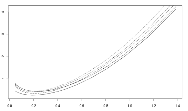
Figure 1: Results of the experiments. The $x$-axis gives the value $g$ where $\lambda=g\sqrt{\log(p)/n}$. The $y$-axis gives $\sum_{i=1}^{n}(\hat{\theta}_{\lambda}^{\prime}X_{i}-\theta^{\prime}X_{i})^{2}$ the error of reconstruction of the signal. The lines code is the following: $\vartheta=-0.95$: solid line, $\vartheta=-0.5$: short dashed line, $\vartheta=0$: dotted line, $\vartheta=0.5$: dot/dash, $\vartheta=0.95$: long dash.

The parameter is given by $\theta=(3,1.5,0,0,2,0,0,\ldots)^{\prime}\in\mathbb{R}^{p}$. This is the toy example used by Tibshirani [30]. Let $\vartheta\in]-1,1[$.

The noise satisfies $\varepsilon_{i}=\vartheta\varepsilon_{i-1}+\eta_{i}$, for $i\geq 2$, where the $\eta_{i}$ are iid $\mathcal{N}(0,1-\vartheta^{2})$ and $\varepsilon_{1}\sim\mathcal{N}(0,1)$. Note that this ensure that $\mathbb{E}(\varepsilon_{i}^{2})=1$ for any $i$, so the noise level does not depent on $\vartheta$. In the experiments,

$$\vartheta\in\{-0.95,-0.5,0,0.5,0.95\}.$$

We fixed a grid of values $\mathcal{G}\subset]0,1.5[$ and we computed, for every experiment, the LASSO estimator with $\lambda=g\sqrt{\log(p)/n}$ for all $g\in\mathcal{G}$. We have repeated the experiment $25$ times for every value of $\vartheta$ and report the results in Figure 1.

We can remark that all the curves are very similar. The minimum reconstruction error is obtained for $g\simeq 0.2$, that corresponds to $\lambda\simeq 0.072$. Note that in the iid case, it is smaller than the theoretical value given by Theorem 2.1, $\lambda=4\sigma\sqrt{2\log(p/\varepsilon)/n}\simeq 2.56$ for $\varepsilon=1/10$, that would correspond to $g\simeq 7.10$, a value that would not event stand in the figure!

5 Application to density estimation

Here we apply Theorem 2.1 and Section 3 to the context of density estimation. Let us remind that in this setting,

$$W_{i}^{(j)}=\mathbb{E}[\varphi_{j}(Z_{1})]-\varphi_{j}(Z_{i}).$$

5.1 Density estimation in the iid case

If the $Z_{i}$ are iid with density $f$ and if $\|\varphi_{j}\|_{\infty}<B$ for any $j\in\{1,\ldots,p\}$ then we can apply Hoeffding inequality [22] to upper bound

$$\left|\int\varphi_{j}(x)f(x)dx-\frac{1}{n}\sum_{i=1}^{n}\varphi_{j}(Z_{i})\right|.$$

We obtain

$$\mathbb{P}\left(\left|\frac{1}{n}\sum_{i=1}^{n}W^{(j)}_{i}\right|\geq\frac{t}{\sqrt{n}}\right)\leq\psi(t)=2\exp(-\frac{t^{2}}{2B^{2}}).$$

So we can apply Theorem 2.1.

Corollary 5.1.

In the context of density estimation, under Assumption ${\bf A}(\kappa)$, if the $Z_{i}$ are iid with density $f$ and if $\|\varphi_{j}\|_{\infty}<B$ for any $j\in\{1,\ldots,p\}$, the choice $\lambda=4B\sqrt{2n\log(2p/\varepsilon)}$ leads to

$$\mathbb{P}\left(\int\left(f_{\hat{\theta}_{\lambda}}(x)-f_{\overline{\theta}}(x)\right)^{2}dx\leq\frac{128B^{2}}{\kappa}\frac{\|\overline{\theta}\|_{0}\log\frac{2p}{\varepsilon}}{n}\right)\geq 1-\varepsilon.$$

This result is essentially known, see [11].

5.2 Density estimation in the dependent case

Note that if as previously we work with bounded $\varphi_{j}(\cdot)$, we automatically have moments of any order. So we will only state a result based on exponential inequality.

So, using Theorem 2.1 and Theorem 3.1 we obtain:

Corollary 5.2.

Let us assume that there are $L>0$ and $B\geq 1$ such that $\varphi_{j}(\cdot)$ is $L$-Lipschitz and $\|\varphi_{j}\|_{\infty}<B$ for any $j\in\{1,\ldots,p\}$. Let us assume that $Z_{1}$, …, $Z_{n}$ satisfy

$$\forall k\geq 0,\quad\sum_{s=0}^{\infty}(s+1)^{k}\eta_{Z}(s)\leq L_{1}L_{2}^{k}(k!)^{\mu}$$

for some $L_{1},L_{2},\mu>0$. Let us put a $c>0$, define

$$\mathcal{C}:=4BLL_{1}+(2^{3+\mu}BL_{1})^{1/(\mu+2)}c$$

and assume that $p$, $n$ and the confidence level $\varepsilon$ are such that

$$p\leq\frac{\varepsilon}{2}\exp\left(\frac{c^{2}n^{\frac{1}{\mu+2}}}{\mathcal{C}}\right).$$

Then

$$\mathbb{P}\left(\int\left(f_{\hat{\theta}_{\lambda}}(x)-f_{\overline{\theta}}(x)\right)^{2}dx\leq\frac{64\,\mathcal{C}}{\kappa}\frac{\|\overline{\theta}\|_{0}\log\left(\frac{2p}{\varepsilon}\right)}{n}\right)\geq 1-\varepsilon.$$ (5.1)

Remark 5.1.

The assumption that the $\varphi_{j}$ are all $L$-Lipschitz for a constant $L$ excludes a lot of interesting dictionaries. If we assume that the $\varphi_{j}$ are $L(n)$-Lipschitz (this would be the case if we used the first $n$ functions in the Fourier basis for example), then we will suffer a loss in (5.1) when compared to the iid case. However, note that Equation (5.2) below is the starting point of our proof, so we cannot hope to find a simple way to remove this hypothesis when using $\eta$-weak dependence. This will be the object of a future work.

Proof.

As $\varphi_{j}$ is $K$-Lipschitz, using Proposition 3.2 we have:

$$\eta_{\varphi_{j}(Z)}(r)\leq L\eta_{Z}(r).$$ (5.2)

So we have

$$\forall k\geq 0,\quad\sum_{k=1}^{\infty}(s+1)^{k}\eta_{\varphi_{j}(Z)}(r)\leq LL_{1}L_{2}^{k}(k!)^{\mu}.$$

Moreover, following Remark 3.3,

$$\left|\mbox{cov }\left(\varphi_{j}(Z_{s_{1}})\cdots\varphi_{j}(Z_{s_{u}}),\varphi_{j}(Z_{t_{1}})\cdots\varphi_{j}(Z_{t_{v}})\right)\right|\leq B^{u+v-1}(u+v)L\cdot\eta_{Z}(r).$$

So we can apply Theorem 3.1 with $\Psi(u,v)=u+v$ and we obtain

$$\mathbb{P}\left(\left|\sum_{i=1}^{n}W_{i}^{(j)}\right|>t\right)\leq 2\exp\left(\frac{-t^{2}/2}{A_{n}+B_{n}^{\frac{1}{\mu+2}}t^{\frac{2\mu+3}{\mu+2}}}\right)$$

with $A_{n}=4nBLL_{1}$ and

$$B_{n}=2^{3+\mu}BL_{1},$$

in other words

$$\mathbb{P}\left(\left|\sum_{i=1}^{n}W_{i}^{(j)}\right|>t\right)\leq 2\exp\left(\frac{-t^{2}/2}{4nBLL_{1}+(2^{3+\mu}BL_{1})^{\frac{1}{\mu+2}}t^{\frac{2\mu+3}{\mu+2}}}\right).$$

We then put $u=t\sqrt{n}$ to obtain

$$\mathbb{P}\left(\left|\frac{1}{n}\sum_{i=1}^{n}W_{i}^{(j)}\right|>\frac{u}{\sqrt{n}}\right)\leq 2\exp\left(\frac{-nu^{2}/2}{4BLL_{1}+(2^{3+\mu}BL_{1})^{\frac{1}{\mu+2}}n^{-\frac{1}{2\mu+4}}u^{\frac{2\mu+3}{\mu+2}}}\right).$$

Here again, if we have

$$u\leq cn^{1/(2\mu+4)}$$

then

$$\mathbb{P}\left(\left|\frac{1}{n}\sum_{i=1}^{n}W_{i}^{(j)}\right|>\frac{u}{\sqrt{n}}\right)\\ \leq 2\exp\left(\frac{-nu^{2}/2}{4BLL_{1}+(2^{3+\mu}BL_{1})^{\frac{1}{\mu+2}}c}\right)2\exp\left(-\frac{nu^{2}}{2\,\mathcal{C}}\right)=:\psi(u).$$

So we take, following Theorem 2.1,

$$\lambda=\frac{4}{\sqrt{n}}\psi^{-1}\left(\frac{\varepsilon}{p}\right)=4\sqrt{\frac{\mathcal{C}\log\left(\frac{2p}{\varepsilon}\right)}{n}}$$

and we obtain, with probability at least $1-\varepsilon$,

$$\int\left(f_{\hat{\theta}_{\lambda}}(x)-f_{\overline{\theta}}(x)\right)^{2}dx\leq\frac{64\,\mathcal{C}}{\kappa}\frac{\|\overline{\theta}\|_{0}\log\left(\frac{2p}{\varepsilon}\right)}{n}.$$

∎

6 Conclusion

In this paper, we showed how the LASSO and other $\ell_{1}$-penalized methods can be extended to the case of dependent random variables.

An open and ambitious question to be adressed later is to find a good data-driven way to calibrate the regularization parameter $\lambda$ when we don’t know in advance the dependence coefficients of our observations.

Anyway this first step with sparsity in the dependent setting is done for accurate applications and our brief simulations let us think that such techniques are reasonable for time series.

Here again extensions to random fields or to dependent point processes seem plausible.

7 Proofs

Proof of Theorem 2.1.

By definition,

$$\frac{1}{n}\sum_{i=1}^{n}Q(Z_{i},\hat{\theta}_{\lambda})+\lambda\|\hat{\theta}_{\lambda}\|_{1}\leq\frac{1}{n}\sum_{i=1}^{n}Q(Z_{i},\overline{\theta})+\lambda\|\overline{\theta}\|_{1}$$

and so

$$R(\hat{\theta}_{\lambda})-R(\overline{\theta})\leq\int_{\mathcal{Z}^{n}}\frac{1}{n}\left\{\sum_{i=1}^{n}\left[Q(z_{i},\hat{\theta}_{\lambda})-Q(z_{i},\overline{\theta})\right]\right\}d\mathbb{P}(z_{1},\ldots,z_{n})\\ -\frac{1}{n}\sum_{i=1}^{n}\left[Q(Z_{i},\hat{\theta}_{\lambda})-Q(Z_{i},\overline{\theta})\right]+\lambda\left(\|\overline{\theta}\|_{1}-\|\hat{\theta}_{\lambda}\|_{1}\right).$$ (7.1)

Now, as $Q$ is quadratic wrt $\theta$ we have, for any $z$,

$$Q(z,\hat{\theta}_{\lambda})=Q(z,\overline{\theta})+(\hat{\theta}_{\lambda}-\overline{\theta})^{\prime}\frac{\partial Q(z,\overline{\theta})}{\partial\theta}+\frac{1}{2}(\hat{\theta}_{\lambda}-\overline{\theta})^{\prime}M(\hat{\theta}_{\lambda}-\overline{\theta}).$$ (7.2)

Moreover, as $\overline{\theta}$ is the minimizer of $R(.)$, we have the relation

$$\frac{\partial R(\overline{\theta})}{\partial\theta}=\int_{\mathcal{Z}^{n}}\frac{1}{n}\sum_{i=1}^{n}\frac{\partial Q(z_{i},\overline{\theta})}{\partial\theta}d\mathbb{P}(z_{1},\ldots,z_{n})=0.$$ (7.3)

Pluging (7.2) and (7.3) into (7.1) leads to

$$R(\hat{\theta}_{\lambda})-R(\overline{\theta})\leq(\hat{\theta}_{\lambda}-\overline{\theta})^{\prime}\frac{1}{n}\sum_{i=1}^{n}\frac{\partial Q(Z_{i},\overline{\theta})}{\partial\theta}+\lambda\left(\|\overline{\theta}\|_{1}-\|\hat{\theta}_{\lambda}\|_{1}\right)$$

and then

$$R(\hat{\theta}_{\lambda})-R(\overline{\theta})\leq\|\hat{\theta}_{\lambda}-\overline{\theta}\|_{1}\sup_{1\leq j\leq p}\left|\frac{1}{n}\sum_{i=1}^{n}\frac{\partial Q(Z_{i},\overline{\theta})}{\partial\theta_{j}}\right|+\lambda\left(\|\overline{\theta}\|_{1}-\|\hat{\theta}_{\lambda}\|_{1}\right).$$ (7.4)

Now, we remind that we have the hypothesis

$$\forall j\in\{1,\ldots,p\},\quad\mathbb{P}\left(\left|\frac{1}{n}\sum_{i=1}^{n}\frac{1}{2}\frac{\partial Q(Z_{i},\overline{\theta})}{\partial\theta_{j}}\right|\geq n^{\alpha-\frac{1}{2}}t\right)\leq\psi(t)$$

that becomes, with a simple union bound argument,

$$\mathbb{P}\left(\sup_{1\leq j\leq p}\left|\frac{1}{n}\sum_{i=1}^{n}\frac{1}{2}\frac{\partial Q(Z_{i},\overline{\theta})}{\partial\theta_{j}}\right|\geq n^{\alpha-\frac{1}{2}}t\right)\leq p\psi(t)$$

and so, if we put $t=\psi^{-1}(\varepsilon/p)$,

$$\mathbb{P}\left(\sup_{1\leq j\leq p}\left|\frac{1}{n}\sum_{i=1}^{n}\frac{1}{2}\frac{\partial Q(Z_{i},\overline{\theta})}{\partial\theta_{j}}\right|\geq n^{\alpha-\frac{1}{2}}\psi^{-1}\left(\frac{\varepsilon}{p}\right)\right)\leq\varepsilon.$$

Also remark that $n^{\alpha-1/2}\psi^{-1}(\varepsilon/p)=\lambda^{*}/4\leq\lambda/4$. So until the end of the proof, we will work on the event

$$\left\{\omega\in\Omega:\sup_{1\leq j\leq p}\left|\frac{1}{n}\sum_{i=1}^{n}\frac{1}{2}\frac{\partial Q(Z_{i}(\omega),\overline{\theta})}{\partial\theta_{j}}\right|\leq\frac{\lambda}{4}\right\}$$

true with probability at least $1-\varepsilon$. Going back to (7.4), we have

$$R(\hat{\theta}_{\lambda})-R(\overline{\theta})\leq\frac{\lambda}{2}\|\hat{\theta}_{\lambda}-\overline{\theta}\|_{1}+\lambda\left(\|\overline{\theta}\|_{1}-\|\hat{\theta}_{\lambda}\|_{1}\right)$$

and then

$$R(\hat{\theta}_{\lambda})-R(\overline{\theta})+\frac{\lambda}{2}\|\hat{\theta}_{\lambda}-\overline{\theta}\|_{1} \leq\lambda\left(\|\hat{\theta}_{\lambda}-\overline{\theta}\|_{1}+\|\overline{\theta}\|_{1}-\|\hat{\theta}_{\lambda}\|_{1}\right)$$

$$=\lambda\left(\sum_{j=1}^{p}|(\hat{\theta}_{\lambda})_{j}-\overline{\theta}_{j}|+\sum_{j=1}^{p}(|\overline{\theta}_{j}|-|(\hat{\theta}_{\lambda})_{j}|)\right)$$

$$=\lambda\left(\sum_{j:\overline{\theta}_{j}\neq 0}|(\hat{\theta}_{\lambda})_{j}-\overline{\theta}_{j}|+\sum_{j:\overline{\theta}_{j}\neq 0}(|\overline{\theta}_{j}|-|(\hat{\theta}_{\lambda})_{j}|)\right)$$

that leads to the following inequality that will play a central role in the end of the proof:

$$R(\hat{\theta}_{\lambda})-R(\overline{\theta})+\frac{\lambda}{2}\|\hat{\theta}_{\lambda}-\overline{\theta}\|_{1}\leq 2\lambda\sum_{j:\overline{\theta}_{j}\neq 0}|(\hat{\theta}_{\lambda})_{j}-\overline{\theta}_{j}|.$$ (7.5)

First, if we remind that $R(\hat{\theta}_{\lambda})-R(\overline{\theta})\geq 0$, (7.5) leads to

$$\|\hat{\theta}_{\lambda}-\overline{\theta}\|_{1}\leq 4\sum_{j:\overline{\theta}_{j}\neq 0}|(\hat{\theta}_{\lambda})_{j}-\overline{\theta}_{j}|$$

and so

$$\sum_{j:\overline{\theta}_{j}=0}|(\hat{\theta}_{\lambda})_{j}-\overline{\theta}_{j}|\leq 3\sum_{j:\overline{\theta}_{j}\neq 0}|(\hat{\theta}_{\lambda})_{j}-\overline{\theta}_{j}|.$$

So we can take $v:=\hat{\theta}_{\lambda}-\overline{\theta}$ in Assumption ${\bf A}(\kappa)$. So, (7.5) leads to

$$R(\hat{\theta}_{\lambda})-R(\overline{\theta})+\frac{\lambda}{2}\|\hat{\theta}_{\lambda}-\overline{\theta}\|_{1} \leq 2\lambda\sum_{j:\overline{\theta}_{j}\neq 0}|(\hat{\theta}_{\lambda})_{j}-\overline{\theta}_{j}|$$ (7.6)

$$\leq 2\lambda\left(\|\overline{\theta}\|_{0}\sum_{j:\overline{\theta}_{j}\neq 0}[(\hat{\theta}_{\lambda})_{j}-\overline{\theta}_{j}]^{2}\right)^{\frac{1}{2}}$$

$$\leq 2\lambda\left(\frac{\|\overline{\theta}\|_{0}}{\kappa}(\hat{\theta}_{\lambda}-\overline{\theta})^{\prime}\frac{\mathbf{M}}{2}(\hat{\theta}_{\lambda}-\overline{\theta})\right)^{\frac{1}{2}}$$

$$=2\lambda\left(\frac{\|\overline{\theta}\|_{0}}{\kappa}\left[R(\hat{\theta}_{\lambda})-R(\overline{\theta})\right]\right)^{\frac{1}{2}}.$$ (7.7)

We conclude that

$$R(\hat{\theta}_{\lambda})-R(\overline{\theta})\leq\frac{4\lambda^{2}\|\overline{\theta}\|_{0}}{\kappa}.$$

Now remark that (7.6) to (7.7) states that a convex quadratic function of $\bigl{[}R(\hat{\theta}_{\lambda})-R(\overline{\theta})\bigr{]}$ is negative, so both roots of that quadratic are real. This leads to

$$\|\hat{\theta}_{\lambda}-\overline{\theta}\|_{1}\leq\frac{2\lambda\|\overline{\theta}\|_{0}}{\kappa}.$$

This ends the proof. ∎

Proof of Proposition 3.3.

First

$$\left|\mathbb{E}(W^{(j)}_{1}+\cdots+W^{(j)}_{n})^{\ell}\right|\leq\ell!A^{(j)}_{\ell,n}\equiv\ell!\sum_{1\leq k_{1},\ldots,k_{\ell}\leq n}\left|\mathbb{E}W^{(j)}_{k_{1}}\cdots W^{(j)}_{k_{\ell}}\right|.$$

The same combinatorial arguments as in [16] yield for $p\leq 2q$

$$A^{(j)}_{\ell,n} \leq C^{(j)}_{q,\ell,n}+\sum_{m=2}^{\ell-2}A^{(j)}_{m,n}A^{(j)}_{\ell-m,n},\mbox{ where}$$ (7.8)

$$C^{(j)}_{q,\ell,n} \equiv (p-1)n\sum_{r=0}^{n-1}(r+1)^{\ell-2}c_{W^{(j)},2q}(r).$$ (7.9)

Let us now assume the condition (3.5) then

$$C^{(j)}_{q,\ell,n} \leq C(\ell-1)n\sum_{r=0}^{n-1}(r+1)^{\ell-2-q}$$

$$\leq C(\ell-1)n\int_{2}^{n+1}x^{\ell-2-q}\,dx,\qquad\mbox{ if }\ell\geq q+2$$

$$\leq C(q+1)(n+1)^{2},\qquad\qquad\qquad\mbox{ if }\ell=q+2$$

$$\leq C\frac{\ell-1}{\ell-q-2}(n+1)^{\ell-q},\ \qquad\qquad\mbox{ if }\ell\geq q+2$$

$$\leq C(\ell-1)n\int_{1}^{n}x^{\ell-2-q}\,dx,\qquad\mbox{ if }\ell<q+2$$

$$\leq C\frac{\ell-1}{q+2-\ell}n.$$

A rough bound is thus $C^{(j)}_{q,\ell,n}\leq C(\ell-1)n^{(\ell-q)\vee 1}$ and we thus derive

$$\begin{array}[]{lllllllll}A^{(j)}_{2,n}&\leq&Cn,&A^{(j)}_{3,n}&\leq&2Cn,&A^{(j)}_{4,n}&\leq&4Cn^{2}\\ A^{(j)}_{5,n}&\leq&8Cn^{2},&A^{(j)}_{6,n}&\leq&17Cn^{3}.\end{array}$$ (7.10)

Now using precisely condition (3.5) with the relation (7.8) we see that if $a_{2}=1$, and $a_{3}=2$ then the sequence recursively defined as

$$a_{m}=m-1+\sum_{k=2}^{m-2}a_{k}a_{m-k}$$ (7.11)

satisfies $A_{m}^{(j)}\leq a_{m}C^{[\frac{m}{2}]}n^{[\frac{m}{2}]}.$ Remember that

$$d_{m}\equiv\frac{1}{m}\frac{(2m-2)!}{((m-1)!)^{2}},\qquad m=2,3,\ldots$$

hence as in [16] we quote that

$$a_{m}\leq d_{m}$$

is less that the $m$-th Catalan number, $d_{m}$ and this ends the proof. ∎

References

- Aka [73] H. Akaike. Information theory and an extension of the maximum likelihood principle. In B. N. Petrov and F. Csaki, editors, 2nd International Symposium on Information Theory, pages 267–281. Budapest: Akademia Kiado, 1973.
- Alq [08] P. Alquier. Density estimation with quadratic loss, a confidence intervals method. ESAIM: P&S, 12:438–463, 2008. \MR2437718
- [3] A. Belloni and V. Chernozhukov. -penalized quantile regression in high-dimensional sparse models. Annals of Statistics, 32(11):2011–2055, 2011.
- [4] A. Belloni and V. Chernozhukov. High dimensional sparse econometric models: An introduction. In P. Alquier, E. Gautier, and G. Stoltz, editors, Inverse Problems and High-Dimensional Estimation. Springer Lecture Notes in Statistics, 2011.
- BGH [09] Y. Baraud, C. Giraud, and S. Huet. Gaussian model selection with an unknown variance. Annals of Statistics, 37(2):630–672, 2009. \MR2502646
- BJMW [10] K. Bartkiewicz, A. Jakubowskin, T. Mikosch, and O. Wintenberger. Infinite variances stable limits for sums of dependent random variables. Probability Theory and Related Fields, 2010.
- BM [01] L. Birgé and P. Massart. Gaussian model selection. Journal of the European Mathematical Society, 3(3):203–268, 2001. \MR1848946
- BRT [09] P. J. Bickel, Y. Ritov, and A. Tsybakov. Simultaneous analysis of lasso and Dantzig selector. Annals of Statistics, 37(4):1705–1732, 2009. \MR2533469
- BTW [07] F. Bunea, A.B. Tsybakov, and M.H. Wegkamp. Aggregation for Gaussian regression. Annals of Statistics, 35:1674–1697, 2007. \MR2351101
- BTWB [10] F. Bunea, A. Tsybakov, M. Wegkamp, and A. Barbu. SPADES and mixture models. Annals of Statistics, 38(4):2525–2558, 2010. \MR2676897
- BWT [07] F. Bunea, M. Wegkamp, and A. Tsybakov. Sparse density estimation with penalties. Proceedings of 20th Annual Conference on Learning Theory (COLT 2007) - Springer, pages 530–543, 2007. \MR2397610
- CDS [01] S. S. Chen, D. L. Donoho, and M. A. Saunders. Atomic decomposition by basis pursuit. SIAM Review, 43(1):129–159, 2001. \MR1639094
- Che [95] S. S. Chen. Basis pursuit, 1995. PhD Thesis, Stanford University.
- CT [07] E. Candes and T. Tao. The Dantzig selector: statistical estimation when is much larger than . Annals of Statistics, 35, 2007. \MR2382644
- DDL+ [07] J. Dedecker, P. Doukhan, G. Lang, J. R. León R., S. Louhichi, and C. Prieur. Weak dependence: with examples and applications, volume 190 of Lecture Notes in Statistics. Springer, New York, 2007. \MR2338725
- DL [99] P. Doukhan and S. Louhichi. A new weak dependence condition and applications to moment inequalities. Stochastic Processes and their Applications, 84(2):313–342, 1999. \MR1719345
- DN [07] P. Doukhan and M. H. Neumann. Probability and moment inequalities for sums of weakly dependent random variables, with applications. Stochastic Processes and their Applications, 117(7):878–903, 2007. \MR2330724
- Dou [94] P. Doukhan. Mixing, volume 85 of Lecture Notes in Statistics. Springer-Verlag, New York, 1994. Properties and examples. \MR1312160
- EHJT [04] B. Efron, T. Hastie, I. Johnstone, and R. Tibshirani. Least angle regression. Annals of Statistics, 32(2):407–499, 2004. \MR2060166
- FHHT [07] J. Friedman, T. Hastie, H. Höfling, and R. Tibshirani. Pathwise coordinate optimization. Annals of Applied Statist., 1(2):302–332, 2007. \MR2415737
- Heb [09] M. Hebiri. Quelques questions de selection de variables autour de l’estimateur lasso, 2009. PhD Thesis, Université Paris 7 (in english).
- Hoe [63] W. Hoeffding. Probability inequalities for sums of bounded random variables. Journal of the American Statistical Association, 58:13–30, 1963. \MR0144363
- [23] V. Koltchinskii. Sparsity in empirical risk minimization. Annales de l’Institut Henri Poincaré, Probabilités et Statistiques, 45(1):7–57, 2009. \MR2500227
- LP [05] H. Leeb and B. M. Pötscher. Sparse estimators and the oracle property, or the return of hodges’ estimator. Cowles Foundation Discussion Papers 1500, Cowles Foundation, Yale University, 2005.
- RBV [08] F. Rapaport, E. Barillot, and J.-P. Vert. Classification of array-CGH data using fused SVM. Bioinformatics, 24(13):1375,1382, 2008.
- Rio [00] E. Rio. Théorie asymptotique pour des processus aléatoire faiblement dépendants. SMAI, Mathématiques et Applications 31, Springer, 2000. \MR2117923
- Ros [56] M. Rosenblatt. A central limit theorem and a strong mixing condition. Proc. Nat. Ac. Sc. U.S.A., 42:43–47, 1956. \MR0074711
- Ros [61] M. Rosenblatt. Independence and dependence. Proceeding 4th. Berkeley Symp. Math. Stat. Prob. Berkeley University Press, pages 411–443, 1961. \MR0133863
- Sch [78] G. Schwarz. Estimating the dimension of a model. Annals of Statistics, 6:461–464, 1978. \MR0468014
- Tib [96] R. Tibshirani. Regression shrinkage and selection via the lasso. Journal of the Royal Statistical Society B, 58(1):267–288, 1996. \MR1379242
- vdGB [09] S. A. van de Geer and P. Bühlmann. On the conditions used to prove oracle results for the lasso. Electronic Journal of Statistics, 3:1360–1392, 2009. \MR2576316
- Win [10] O. Wintenberger. Deviation inequalities for sums of weakly dependent time series. Electronic Communications in Probability, 15:489–503, 2010. \MR2733373
- ZH [05] H. Zou and T. Hastie. Regularization and variable selection via the elastic net. Journal of the Royal Statistical Society B, 67(2):301–320, 2005. \MR2137327