Theory of Forces Induced by

Evanescent Fields

M. Nieto-Vesperinas and J. R. Arias-González

¹Instituto de Ciencia de Materiales de Madrid, CSIC

²Instituto Madrileño de Estudios Avanzados en Nanociencia

Cantoblanco, 28049 Madrid, Spain.

1 Introduction

The purpose of this report is to present the theoretical foundations of the interaction of evanescent fields on an object. Evanescent electromagnetic waves are inhomogeneous components of the near field, bound to the surface of the scattering object. These modes travel along the illuminated sample surface and exponentially decrease outside it [Born 99a, Nieto-Vesperinas 91, Mandel 95], e.g., either in the form of lateral waves [Tamir 72a, Tamir 72b] created by total internal reflection (TIR) at dielectric flat interfaces, whispering–gallery modes in dielectric tips and particles [Hill 88, Owen 81, Benincasa 87, Collot 93, Knight 95, Weiss 95, Nieto-Vesperinas 96] or of plasmon polaritons [Raether 88] in metallic corrugated interfaces (see Section 5). The force exerted by these evanescent waves on particles near the surface is of interest for several reasons. On the one hand, evanescent waves convey high resolution of the scattered field signal, beyond the half wavelength limit. This is the essence of near–field scanning optical microscopy, abbreviated usually as NSOM [Pohl 93, Paesler 96]. These fields may present large concentrations and intensity enhancements in subwavelength regions near tips thus giving rise to large gradients that produce enhanced trapping forces that may enable one to handle particles within nanometric distances [Novotny 97]. In addition, the large contribution of evanescent waves to the near field is the basis of the high resolution of signals obtained by transducing the force due to these waves on particles over surfaces when such particles are used as probes. On the other hand, evanescent waves have been used both to control the position of a particle above a surface and to estimate the interaction (colloidal force) between such a particle and the surface (see Chapter 6) [Sasaki 97, Clapp 99, Dogariu 00].

The first experimental observation, demonstrating the mechanical action of a single evanescent wave (i.e., of the lateral wave produced by total internal reflection at a dielectric (saphire–water interface) on microspheres immersed in water over a dielectric surface) was made in [Kawata 92]. Further experiments either over waveguides [Kawata 96] or attaching the particle to the cantilever of an atomic force microscope (AFM) [Vilfan 98] aimed at estimating the magnitude of this force.

The scattering of an evanescent electromagnetic wave by a dielectric sphere has been investigated by several authors using Mie’s scattering theory (addressing scattering cross sections [Chew 79] and electromagnetic forces [Almaas 95]), as well as using ray optics [Prieve 93, Walz 99]. In particular, [Walz 99] made a comparison with [Almaas 95]. Although no direct evaluation of either theoretical work with any experimental result has been carried out yet, likely due to the yet lack of accurate well characterized and controlled experimental estimations of these TIR observed forces. In fact, to get an idea of the difficulties of getting accurate experimental data, we should consider the fluctuations of the particle position in its liquid environment, due to both Brownian movement and drift microcurrents, as well as the obliteration produced by the existence of the friction and van der Waals forces between particle and surface [Vilfan 98, Almaas 95]. This has led so far to discrepancies between experiment and theory.

In the next section we shall address the effect of these forces on particles from the point of view of the dipolar approximation, which is of considerable interpretative value to understand the contribution of horizontal and vertical forces. Then we shall show how the multiple scattering of waves between the surface and the particle introduces important modifications of the above mentioned forces, both for larger particles and when they are very close to substrates. Further, we shall investigate the interplay of these forces when there exists slight corrugation in the surface profile. Then the contribution of evanescent waves created under total internal reflection still being important, shares its effects with radiative propagating components that will exert scattering repulsive forces. Even so, the particle can be used in these cases as a scanning probe that transduces this force in a photonic force microscopy operation.

2 Force on a Small Particle:
The Dipolar Approximation

Small polarizable particles, namely, those with radius $a\ll\lambda$, in the presence of an electromagnetic field experience a Lorentz force [Gordon 73]:

$${\bf F}=({\vec{\wp}}\cdot\nabla){\vec{{\cal E}}}+\frac{1}{c}\frac{\partial{\vec{\wp}}}{\partial t}\times{\vec{{\cal B}}}.$$ (1)

In Equation (1) ${\vec{\wp}}$ is the induced dipole moment density of the particle, and ${\vec{{\cal E}}}$, ${\vec{{\cal B}}}$ are the electric and magnetic vectors, respectively.

At optical frequencies, used in most experiments, the observed magnitude of the electromagnetic force is the time–averaged value. Let the electromagnetic field be time–harmonic, so that ${\vec{{\cal E}}}({\bf r},t)=\Re e\{{\bf E}({\bf r})\exp(-i\omega t)\}$, ${\vec{{\cal B}}}({\bf r},t)=\Re e\{{\bf B}({\bf r})\exp(-i\omega t)\}$, ${\vec{\wp}}({\bf r},t)=\Re e\{{\bf p}({\bf r})\exp(-i\omega t)\}$; ${\bf E}({\bf r})$, ${\bf B}({\bf r})$ and ${\bf p}({\bf r})$ being complex functions of position in the space, and $\Re e$ denoting the real part. Then, the time–averaged Lorentz force over a time interval $T$ large compared to $2\pi/\omega$ [Born 99b] is

$$\langle{\bf F}({\bf r})\rangle=\frac{1}{4T}\int_{-T/2}^{T/2}dt\left[{{{{{({\bf p}+{\bf p}^{\ast})\cdot\nabla({\bf E}+{\bf E}^{\ast})+\frac{1}{c}\left(\frac{\partial{\bf p}}{\partial t}+\frac{\partial{\bf p}^{\ast}}{\partial t}\right)\times({\bf B}+{\bf B}^{\ast})}}}}}\right],$$ (2)

where $\ast$ denotes complex conjugate. On substituting in Equation (2) ${\bf E}$, ${\bf B}$, and ${\bf p}$ by their time harmonic expressions given above and performing the integral, one obtains for each $i^{th}$–Cartesian component of the force

$$\langle F_{j}({\bf r})\rangle=\frac{1}{2}\Re e\left\{p_{k}\frac{\partial E_{j}^{\ast}({\bf r})}{\partial x_{k}}+\frac{1}{c}\epsilon_{jkl}\frac{\partial p_{k}}{\partial t}B_{l}^{\ast}\right\}.$$ (3)

In Equation (3) $j=1,2,3$, $\epsilon_{jkl}$ is the completely antisymmetric Levy–Civita tensor. On using the Maxwell equation ${\bf B}=(c/i\omega)\nabla\times{\bf E}$ and the relationships ${\bf p}=\alpha{\bf E}$ and $\partial{\bf p}/\partial t=-i\omega{\bf p}$, $\alpha$ being the particle polarizability, Equation (3) transforms into

$$\langle F_{j}({\bf r})\rangle=\frac{1}{2}\Re e\left\{{{{{{\alpha\left(E_{k}\frac{\partial E_{j}^{\ast}({\bf r})}{\partial x_{k}}+\epsilon_{jkl}~{}\epsilon_{lmn}E_{k}\frac{\partial E_{n}^{\ast}}{\partial x_{m}}\right)}}}}}\right\}.$$ (4)

Since $\epsilon_{jkl}\epsilon_{lmn}=\delta_{jm}\delta_{kn}-\delta_{jn}\delta_{km}$, one can finally express the time–averaged Lorentz force on the small particle as [Chaumet 00c]

$$\langle F_{j}({\bf r})\rangle=\frac{1}{2}\Re e\left\{{{{{{\alpha E_{k}\frac{\partial E_{k}^{\ast}({\bf r})}{\partial x_{j}}}}}}}\right\}.$$ (5)

Equation (5) constitutes the expression of the time–averaged force on a particle in an arbitrary time–harmonic electromagnetic field.

For a dipolar particle, the polarizability is [Draine 88]

$$\alpha=\frac{\alpha_{0}}{1-\frac{2}{3}ik^{3}\alpha_{0}}.$$ (6)

In Equation (6) $\alpha_{0}$ is given by: $\alpha_{0}=a^{3}(\epsilon-1)/(\epsilon+2)$, $\epsilon=\epsilon_{2}/\epsilon_{0}$ being the dielectric permittivity contrast between the particle, $\epsilon_{2}$, and the surrounding medium, $\epsilon_{0}$; and $k=\sqrt{\epsilon_{0}}k_{0}$, $k_{0}=\omega/c$. For $ka\ll 1$, one can approximate $\alpha$ by: $\alpha=\alpha_{0}(1+\frac{2}{3}ik^{3}|\alpha_{0}|^{2})$. The imaginary part in this expression of $\alpha$ constitutes the radiation–reaction term.

The light field can be expressed by its paraxial form, e.g., it is a beam or a plane wave, either propagating or evanescent, so that it has a main propagation direction along ${\bf k}$, the light electric vector will then be described by

$${\bf E}({\bf r})={\bf E}_{0}({\bf r})\exp(i{\bf k}\cdot{\bf r}).$$ (7)

Substituting Equation (7) into Equation (5), one obtains for the force

$$\langle{\bf F}\rangle=\frac{1}{4}\Re e\{\alpha\}\nabla|{\bf E}_{0}|^{2}+\frac{1}{2}{\bf k}\Im m\{\alpha\}|{\bf E}_{0}|^{2}-\frac{1}{2}\Im m\{\alpha\}\Im m\{{\bf E}_{0}\cdot\nabla{\bf E}_{0}^{\ast}\},$$ (8)

where $\Im m$ denotes imaginary part. The first term is the gradient force acting on the particle, whereas the second term represents the radiation pressure contribution to the scattering force that, on substituting the above approximation for $\alpha$, namely, $\alpha=\alpha_{0}(1+\frac{2}{3}ik^{3}|\alpha_{0}|^{2})$, can also be expressed for a Rayleigh particle ($ka\ll 1$) as [van de Hulst 81] $(|{\bf E}_{0}|^{2}/8\pi)C{\bf k}/k$, where $C$ is the particle scattering cross section given by $C=(8/3)\pi k^{4}|\alpha_{0}|^{2}$. Notice that the last term of Equation (8) is only zero when either $\alpha$ or ${\bf E}_{0}$ is real. (This is the case for a plane propagating or evanescent wave but not for a beam, in general.)

3 Force on a Dipolar Particle due to
an Evanescent Wave

Let the small particle be exposed to the electromagnetic field of an evanescent wave, whose electric vector is ${\bf E}={\bf T}\exp(-qz)\exp(i{\bf K}\cdot{\bf R})$, where we have written ${\bf r}=({\bf R},z)$ and ${\bf k}=({\bf K},k_{z})$, ${\bf K}$ and $k_{z}$ satisfying $K^{2}+k_{z}^{2}=k^{2}$, $k^{2}=\omega^{2}\epsilon_{0}/c^{2}$, with $k_{z}=iq=i\sqrt{K^{2}-k_{0}^{2}}$. This field is created under total internal reflection at a flat interface ($z=$ constant, below the particle) between two media of dielectric permittivity ratio $\epsilon_{0}/\epsilon_{1}$ (see also inset of Figure 2(a)). The incident wave, either $s$ or $p$ polarized, (i.e., with the electric vector either perpendicular or in the plane of incidence: the plane formed by the incident wavevector ${\bf k}_{i}$ at the interface and the surface normal $\hat{z}$) enters from the denser medium at $z<0$. The particle is in the medium at $z>0$. Without loss of generality, we shall choose the incidence plane as $OXZ$, so that ${\bf K}=(K,0)$. Let $T_{\perp}$ and $T_{\parallel}$ be the transmitted amplitudes into $z>0$ for $s$ and $p$ polarizations, respectively. The electric vector is:

$${\bf E}=(0,1,0){T_{\perp}}\exp(iKx)\exp(-qz),$$ (9)

for $s$ polarization, and

$${\bf E}=(-iq,0,K)\frac{T_{\parallel}}{k}\exp(iKx)\exp(-qz).$$ (10)

for $p$ polarization

By introducing the above expressions for the electric vector ${\bf E}$ into Equation (8), we readily obtain the average total force on the particle split into the scattering and gradient forces. The scattering force is contained in the $OXY$–plane (that is, the plane containing the propagation wavevector of the evanescent wave), namely,

$$\langle F_{x}\rangle=\frac{|T|^{2}}{2}K\Im m\{\alpha\}\exp(-2qz);$$ (11)

For the gradient force, which is purely directed along $OZ$, one has

$$\langle F_{z}\rangle=-\frac{|T|^{2}}{2}q\Re e\{\alpha\}\exp(-2qz).$$ (12)

In Equations (11) and (12) $T$ stands for either $T_{\perp}$ or $T_{\parallel}$, depending on whether the polarization is $s$ or $p$, respectively.

For an absorbing particle, on introducing Equation (6) for $\alpha$ into Equations (11) and (12), one gets for the scattering force

$$\langle F_{x}\rangle=\frac{|T|^{2}}{2}K\exp(-2qz)\frac{\Im m\{\alpha_{0}\}+(2/3)k^{3}|\alpha_{0}|^{2}}{1+(4/9)k^{6}|\alpha_{0}|^{2}},$$ (13)

and for the gradient force

$$\langle F_{z}\rangle=-\frac{|T|^{2}}{2}q\frac{\Re e\{\alpha_{0}\}}{1+(4/9)k^{6}|\alpha_{0}|^{2}}\exp(-2qz).$$ (14)

It should be remarked that, except near resonances, in general $\Im m\{\alpha_{0}\}$ is a positive quantity and therefore the scattering force in Equation (13) is positive in the propagation direction $K$ of the evanescent wave, thus pushing the particle parallel to the surface, whereas the gradient force Equation (14) is negative or positive along $OZ$, therefore, attracting or repelling the particle towards the surface, respectively, according to whether $\Re e\{\alpha\}>0$ or $\Re e\{\alpha\}<0$. The magnitudes of these forces increase with the decrease of distance to the interface and it is larger for $p$ polarization since in this case the dipoles induced by the electric vector at both the particle and the surface are oriented parallel to each other, thus resulting in a smaller interaction than when these dipoles are induced in the $OXZ$–plane ($s$–polarization) [Alonso 68].

In particular, if $ka\ll 1$, Equation (13) becomes

$$\langle F_{x}\rangle=\frac{|T|^{2}}{2}K\exp(-2qz)\left[a^{3}\Im m\left\{\frac{\epsilon-1}{\epsilon+2}\right\}+\frac{2}{3}k^{3}a^{6}\left|\frac{\epsilon-1}{\epsilon+2}\right|^{2}\right];$$ (15)

The first term of Equation (15) is the radiation pressure of the evanescent wave on the particle due to absorption, whereas the second term corresponds to scattering. This expression can be further expressed as

$$\langle F_{x}\rangle=\frac{|T|^{2}}{8\pi}\frac{K}{k}\exp(-2qz)~{}C_{ext}.$$ (16)

where the particle extinction cross section $C_{ext}$ has been introduced as

$$C_{ext}=4\pi ka^{3}\Im m\left\{\frac{\epsilon-1}{\epsilon+2}\right\}+\frac{8\pi}{3}k^{4}a^{6}\left|\frac{\epsilon-1}{\epsilon+2}\right|^{2}.$$ (17)

Notice that Equation (17) coincides with the value obtained from Mie’s theory for small particles in the low–order expansion of the size parameter $ka$ of the extinction cross section [van de Hulst 81].

Although the above equations do not account either for multiple scattering as described by Mie’s theory for larger particles or for multiple interactions of the wave between the particle and the dielectric surface, they are useful to understand the fundametals of the force effects induced by a single evanescent wave on a particle. It should be remarked, however, that as shown at the end of this section, once Mie’s theory becomes necessary, multiple scattering with the surface demands that its contribution be taken into account.

Figure 1: Forces in the $Z$ direction and in the $X$ direction (as insets) acting on a sphere with radius $a=60$ $nm$, in the dipolar approximation. The angle of incidence is $\theta_{0}=42^{o}$, larger than the critical angle $\theta_{c}=41.8^{o}$ (for the glass–air interface). $\lambda=632.8$ $nm$. Solid lines: $s$ polarization, dashed lines: $p$ polarization. The sphere material is: (a): glass, (b): silicon, (c): gold.

Figure 1 shows the evolution of the scattering and gradient forces on three kinds of particles, namely, glass ($\epsilon_{2}=2.25$), silicon ($\epsilon_{2}=15+i0.14$) and gold ($\epsilon_{2}=-5.65+i0.75$), all of radius $a=60$ $nm,$ as functions of the gap distance $d$ between the particle and the surface at which the evanescent wave is created. The illuminating evanescent wave is due to refraction of an incident plane wave of power $P=\frac{c\sqrt{\epsilon_{1}}}{8\pi}|A|^{2}=1.9\times 10^{-2}$ $mW/\mu m^{2}$, equivalent to $150$ $mW$ over a circular section of radius $50$ $\mu m$, on a glass–air interface at angle of incidence $\theta_{0}=42^{o}$ and $\lambda=632.8$ $nm$ (the critical angle is $\theta_{c}=41.8^{o}$), both at $s$ and $p$ polarization (electric vector perpendicular and parallel, respectively, to the incidence plane at the glass–air interface, namely, $|T_{\perp}|^{2}=4\epsilon_{1}\cos^{2}\theta_{0}|A|^{2}/(\epsilon_{1}-1)$, $|T_{\parallel}|^{2}=4\epsilon_{1}\cos^{2}\theta_{0}|A|^{2}/[(\epsilon_{1}-1)((1+\epsilon_{1})\sin^{2}\theta_{0}-1)]$).

These values of forces are consistent with the magnitudes obtained on similar particles by applying Maxwell’s stress tensor (to be discussed in Section 4.1) via Mie’s scattering theory [Almaas 95]. However, as shown in the next section, as the size of the particle increases, the multiple interaction of the illuminating wave between the particle and the substrate cannot be neglected. Therefore, the above results, although of interpretative value, should be taken with care at distances smaller than $10$ $nm$, since in that case multiple scattering makes the force stronger. This will be seen next.

4 Influence of Interaction with the Substrate

Among the several studies on forces of evanescent waves over particles, there are several models which calculate the forces from Maxwell’s stress tensor on using Mie’s theory to determine the scattered field in and around the sphere, without, however, taking into account the multiple scattering between the interface at which the evanescent wave is created and the sphere [Almaas 95, Chang 94, Walz 99]. We shall next see that, except at certain distances, this multiple interaction cannot be neglected.

The equations satisfied by the electric and magnetic vectors in a non–magnetic medium are

$$\nabla\times\nabla\times{\bf E}-k^{2}{\bf E} = 4\pi k^{2}{\bf P},$$ (18)

$$\nabla\times\nabla\times{\bf H}-k^{2}{\bf H} = -i4\pi k\nabla\times{\bf P},$$ (19)

where ${\bf P}$ is the polarization vector. The solutions to Equations (18) and (19) are written in integral form as

$${\bf E}({\bf r}) = k^{2}\int d^{3}r^{\prime}~{}{\bf P}({\bf r}^{\prime})\cdot\overset{\leftrightarrow}{{\cal G}}({\bf r},{\bf r}^{\prime}),$$ (20)

$${\bf H}({\bf r}) = -ik\int d^{3}r^{\prime}~{}\nabla\times{\bf P}({\bf r}^{\prime})\cdot\overset{\leftrightarrow}{{\cal G}}({\bf r},{\bf r}^{\prime}),$$ (21)

In Equations (20) and (21) $\overset{\leftrightarrow}{{\cal G}}({\bf r},{\bf r}^{\prime})$ is the outgoing Green’s dyadic or field created at ${\bf r}$ by a point dipole at ${\bf r}^{\prime}$. It satisfies the equation

$$\nabla\times\nabla\times\overset{\leftrightarrow}{{\cal G}}({\bf r},{\bf r}^{\prime})-k^{2}\overset{\leftrightarrow}{{\cal G}}({\bf r},{\bf r}^{\prime})=4\pi\delta({\bf r}-{\bf r}^{\prime})\overset{\leftrightarrow}{{\cal I}}.$$ (22)

Let’s introduce the electric displacement vector ${\bf D}={\bf E}+4\pi{\bf P}$. Then,

$$\nabla\times\nabla\times{\bf E}=\nabla\times\nabla\times{\bf D}-4\pi\nabla\times\nabla\times{\bf P}.$$ (23)

Using the vectorial identity $\nabla\times\nabla\times{\bf D}=\nabla(\nabla\cdot{\bf D})-\nabla^{2}{\bf D}$, and the fact that in the absence of free charges, $\nabla\cdot{\bf D}=0$, it is easy to obtain

$$\nabla\times\nabla\times{\bf E} = -\nabla^{2}{\bf D}-4\pi\left[\nabla(\nabla\cdot{\bf P})-\nabla^{2}{\bf P}\right]$$ (24)

$$= -\nabla^{2}{\bf E}-4\pi\nabla(\nabla\cdot{\bf P}),$$ (25)

which straightforwardly transforms Equation (18) into:

$$\nabla^{2}{\bf E}+k^{2}{\bf E}=-4\pi[k^{2}{\bf P}+\nabla(\nabla\cdot{\bf P})],$$ (26)

whose solution is

$${\bf E}({\bf r})=k^{2}\int d^{3}r^{\prime}~{}[{\bf P}+\nabla(\nabla\cdot{\bf P})]({\bf r}^{\prime})~{}G({\bf r},{\bf r}^{\prime})\,.$$ (27)

In a homogenous infinite space the function $G$ of Equation (27) is $G_{0}({\bf r},{\bf r}^{\prime})=\exp(ik|{\bf r}-{\bf r}^{\prime}|)/|{\bf r}-{\bf r}^{\prime}|$, namely, a spherical wave, or scalar Green’s function, corresponding to radiation from a point source at ${\bf r}^{\prime}$.

To determine $\overset{\leftrightarrow}{{\cal G}}$, we consider the case in which the radiation comes from a dipole of moment ${\bf p}$, situated at ${\bf r}_{0}$; the polarization vector ${\bf P}$ is expressed as

$${\bf P}({\bf r})={\bf p}\delta({\bf r}-{\bf r}_{0}).$$ (28)

Introducing Equation (28) into Equation (27) one obtains the well known expression for the electric field radiated by a dipole

$${\bf E}({\bf r})=k^{2}{\bf p}\nabla({\bf p}\cdot\nabla)\frac{\exp(ik|{\bf r}-{\bf r}^{\prime}|)}{|{\bf r}-{\bf r}^{\prime}|}.$$ (29)

On the other hand, if Equation (28) is introduced into Equation (20) one obtains

$${\bf E}({\bf r})=k^{2}{\bf p}\cdot\overset{\leftrightarrow}{{\cal G}}_{0}({\bf r},{\bf r}^{\prime}).$$ (30)

On comparing Equations (29) and (30), since both give identical value for ${\bf E}$, we get

$$k^{2}{\bf P}({\bf r}^{\prime})\cdot\overset{\leftrightarrow}{{\cal G}}_{0}({\bf r},{\bf r}^{\prime})=[k^{2}{\bf p}\nabla({\bf p}\cdot\nabla)]G_{0}({\bf r},{\bf r}^{\prime}),$$ (31)

i.e., the tensor Green’s function in a homogenous infinite space is

$$\overset{\leftrightarrow}{{\cal G}}_{0}({\bf r},{\bf r}^{\prime})=\left(\overset{\leftrightarrow}{{\cal I}}+\frac{1}{k^{2}}\nabla\nabla\right)G_{0}({\bf r},{\bf r}^{\prime}).$$ (32)

A remark is in order here. When applying Equation (32) in calculations one must take into account the singularity at ${\bf r}={\bf r}^{\prime}$, this is accounted for by writing $\overset{\leftrightarrow}{{\cal G}}_{0}$ as [Yaghjian 80]:

$$\overset{\leftrightarrow}{{\cal G}}_{0}({\bf r},{\bf r}^{\prime})={\cal P}\left[{{{{{{{{\ \left(\overset{\leftrightarrow}{{\cal I}}+\frac{1}{k^{2}}\nabla\nabla\right)G_{0}({\bf r},{\bf r}^{\prime})}}}}}}}}\right]-\frac{1}{k^{2}}\delta({\bf r}-{\bf r}^{\prime})\overset{\leftrightarrow}{{\bf L}}_{v}.$$ (33)

In Equation (33) ${\cal P}$ represents the principal value and $\overset{\leftrightarrow}{{\bf L}}_{v}$ is a dyadic that describes the singularity and corresponds to an exclusion volume around ${\bf r}={\bf r}^{\prime}$, on whose shape it depends [Yaghjian 80].

4.1 The Coupled Dipole Method

Among the several methods of calculating multiple scattering between bodies of arbitrary shape (e.g., transition matrix, finite–difference time domain, integral procedures, discrete dipole approximation, etc.) we shall next address the coupled dipole method (Purcell and Pennipacker [Purcell73]). This procedure is specially suitable for multiple scattering between a sphere and a flat interface.

Let us return to the problem of determining the interaction of the incident wave with the substrate and the sphere. The scattered electromagnetic field is obtained from the contribution of all polarizable elements of the system under the action of the illuminating wave. The electric vector above the interface is given by the sum of the incident field ${\bf E}_{i}$ and that expressed by Equation (20) with the dyadic Green function $\overset{\leftrightarrow}{{\cal G}}$ being given by

$$\overset{\leftrightarrow}{{\cal G}}({\bf r},{\bf r}^{\prime})=\overset{\leftrightarrow}{{\cal G}}_{0}({\bf r},{\bf r}^{\prime})+\overset{\leftrightarrow}{{\cal G}}_{s}({\bf r},{\bf r}^{\prime}).$$ (34)

In Equation (34) $\overset{\leftrightarrow}{{\cal G}}_{0}$ is given by Equation (32) and, as such, it corresponds to the field created by a dipole in a homogeneous infinite space. On the other hand, $\overset{\leftrightarrow}{{\cal G}}_{s}$ represents the field from the dipole after reflection at the interface.

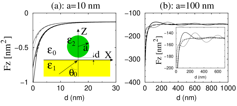
Figure 2: Normalized force in the $Z$ direction acting on a glass sphere on a glass–vacuum interface. The angle of incidence $\theta_{0}=42^{o}$ is larger than the critical angle $\theta_{c}=41.8^{o}$. $\lambda=632.8$ $nm$. Thin lines: $S$ polarization, Thick lines: $P$ polarization. (a): $a=10$ $nm$, full line: dipole approximation, dashed line: CDM–A, dotted line: CDM–B. The inset shows the scattering geometry. (b): $a=100$ $nm$, full line: calculation with CDM–B, dashed line: static approximation. (From Ref. [Chaumet 00a]).

The polarization vector ${\bf P}$ is represented by the collection of $N$ dipole moments ${\bf p}_{j}$ corresponding to the $N$ polarizable elements of all materials included in the illuminated system, namely,

$${\bf P}({\bf r})=\sum_{j}^{N}{\bf p}_{j}\delta({\bf r}-{\bf r}_{i}).$$ (35)

The relationship between the $k^{{\rm th}}$ dipole moment ${\bf p}_{k}$ and the exciting electric field is, as before, given by ${\bf p}_{k}=\alpha_{k}{\bf E}({\bf r}_{k})$, with $\alpha_{k}$ expressed by Equation (6). Then, Equations (27), (34) and (35) yield

$${\bf E}({\bf r}_{j})=k^{2}\sum_{k}^{N}\alpha_{k}[\overset{\leftrightarrow}{{\cal G}}_{0}({\bf r}_{j},{\bf r}_{k})+\overset{\leftrightarrow}{{\cal G}}_{s}({\bf r}_{j},{\bf r}_{k})]\cdot{\bf E}({\bf r}_{k}).$$ (36)

The determination of $\overset{\leftrightarrow}{{\cal G}}_{s}$ either above or below the flat interface is discussed next (one can find more details in Ref. [Agarwal 75a]). Let us summarize the derivation of its expression above the surface. The field ${\bf E}$ in the half–space $z>0$, from a dipole situated in this region, is the sum of that from the dipole in free space and the field ${\bf E}_{r}$ produced on reflection of the latter at the interface. Taking Equation (30) into account, this is therefore

$${\bf E}({\bf r})=k^{2}{\bf p}\cdot\overset{\leftrightarrow}{{\cal G}}_{0}({\bf r},{\bf r}^{\prime})+{\bf E}_{r}({\bf r}),\text{ \ \ \ }z>0\,.$$ (37)

Both the spherical wave $G_{0}$ and ${\bf E}_{r}$ are expanded into plane waves. The former is, according to Weyl’s representation [Baños 66a, Nieto-Vesperinas 91],

$$G_{0}({\bf r},{\bf r}^{\prime})=\frac{i}{2\pi}\int_{-\infty}^{\infty}\frac{d^{2}K}{k_{z}({\bf K})}\exp[i({\bf K}\cdot({\bf R}-{\bf R}^{\prime})+k_{z}|z-z^{\prime}|)]\,.$$ (38)

On the other hand, ${\bf E}_{r}$ is expanded as an angular spectrum of plane waves [Nieto-Vesperinas 91, Mandel 95]

$${\bf E}_{r}({\bf r})=\int_{-\infty}^{\infty}d^{2}K~{}{\bf A}_{r}({\bf K})\exp[i({\bf K}\cdot{\bf R}+k_{z}z)].$$ (39)

Introducing Equation (38) into Equation (34) one obtains a plane wave expansion for $\overset{\leftrightarrow}{{\cal G}}_{0}$. This gives the plane wave components ${\bf A}_{h}({\bf K})$ of the first term of Equation (37). Then, the plane wave components ${\bf A}_{r}({\bf K})$ of the second term of Equation (37) are given by

$${\bf A}_{r}({\bf K})=r({\bf K}){\bf A}_{h}({\bf K}),$$ (40)

In Equation (40) $r({\bf K})$ is the Fresnel reflection coefficient corresponding to the polarization of ${\bf A}_{h}$. The result is therefore that $\overset{\leftrightarrow}{{\cal G}}$, Equation (34), is

$$\overset{\leftrightarrow}{{\cal G}}({\bf r},{\bf r}^{\prime})=\frac{1}{4\pi^{2}}\int_{-\infty}^{\infty}d^{2}K~{}{\overset{\leftrightarrow}{{\bf S}}}^{-1}({\bf K})\cdot\overset{\leftrightarrow}{{\bf g}}({\bf K},z,z^{\prime})\cdot\overset{\leftrightarrow}{{\bf S}}({\bf K})\exp[i{\bf K}\cdot({\bf R}-{\bf R}^{\prime})],$$ (41)

where [Agarwal 75a, Agarwal 75b, Keller 93]

$$\overset{\leftrightarrow}{{\bf S}}({\bf K})=\frac{1}{K}\left(\begin{array}[]{ccc}k_{x}&k_{y}&0\\ -k_{y}&k_{x}&0\\ 0&0&K\end{array}\right),$$ (42)

and the dyadic $\overset{\leftrightarrow}{{\bf g}}$ has the elements [Greffet 97]

$$g_{11} = \frac{-ik_{z}^{(0)}}{2\epsilon_{0}k_{0}^{2}}\left[\frac{\epsilon_{0}k_{z}^{(1)}-\epsilon_{1}k_{z}^{(0)}}{\epsilon_{0}k_{z}^{(1)}+\epsilon_{1}k_{z}^{(0)}}\exp[ik_{z}^{(0)}(z+z^{\prime})]+\exp(ik_{z}^{(0)}|z-z^{\prime}|)\right],$$ (43)

$$g_{22} = \frac{-i}{2k_{z}^{(0)}}\left[{{{{{\frac{k_{z}^{(0)}-k_{z}^{(1)}}{k_{z}^{(0)}+k_{z}^{(1)}}\exp[ik_{z}^{(0)}(z+z^{\prime})]+\exp(ik_{z}^{(0)}|z-z^{\prime}|)}}}}}\right],$$ (44)

$$g_{33} = \frac{iK^{2}}{2\epsilon_{0}k_{z}^{(0)}k_{0}^{2}}\left[\frac{\epsilon_{0}k_{z}^{(1)}-\epsilon_{1}k_{z}^{(0)}}{\epsilon_{0}k_{z}^{(1)}+\epsilon_{1}k_{z}^{(0)}}\exp[ik_{z}^{(0)}(z+z^{\prime})]-\exp(ik_{z}^{(0)}|z-z^{\prime}|)\right]$$ (45)

$$+ \frac{1}{\epsilon_{0}k_{0}^{2}}\delta(z-z^{\prime}),$$

$$g_{12} = 0,$$ (46)

$$g_{13} = \frac{-iK}{2\epsilon_{0}k_{0}^{2}}\left[\frac{\epsilon_{0}k_{z}^{(1)}-\epsilon_{1}k_{z}^{(0)}}{\epsilon_{0}k_{z}^{(1)}+\epsilon_{1}k_{z}^{(0)}}\exp[ik_{z}^{(0)}(z+z^{\prime})]-\exp(ik_{z}^{(0)}|z-z^{\prime}|)\right],$$ (47)

$$g_{31} = \frac{iK}{2\epsilon_{0}k_{0}^{2}}\left[\frac{\epsilon_{0}k_{z}^{(1)}-\epsilon_{1}k_{z}^{(0)}}{\epsilon_{0}k_{z}^{(1)}+\epsilon_{1}k_{z}^{(0)}}\exp[ik_{z}^{(0)}(z+z^{\prime})]+\exp(ik_{z}^{(0)}|z-z^{\prime}|)\right].$$ (48)

We have used $k_{z}^{(j)}=iq_{j}=(K^{2}-\epsilon_{j}k_{0}^{2})^{1/2}$, $j=0$ ,$1$, and $k_{0}=\omega/c$. To determine the force acting on the particle, we also need the magnetic field. This is found by the relationships ${\bf B}({\bf r})=-i/k\nabla\times{\bf E}({\bf r})$. Then the time–averaged force obtained from Maxwell’s stress tensor $\overset{\leftrightarrow}{{\bf T}}$ [Stratton 41, Jackson 75] is

$$\langle{\bf F}\rangle=\int_{S}d^{2}r~{}\left\langle\overset{\leftrightarrow}{{\bf T}}({\bf r})\right\rangle\cdot{\bf n}.$$ (49)

Equation (49) represents the flow of the time–average of Maxwell’s stress tensor $\langle\overset{\leftrightarrow}{{\bf T}}\rangle$ across a surface $S$ enclosing the particle, ${\bf n}$ being the local outward normal. The elements $T_{\alpha\beta}$ are [Jackson 75]

$$\left\langle T_{\alpha\beta}({\bf r})\right\rangle=\frac{1}{8\pi}\left[E_{\alpha}E_{\beta}^{\ast}+B_{\alpha}B_{\beta}^{\ast}-\frac{1}{2}({\bf E}\cdot{\bf E}^{\ast}+{\bf B}\cdot{\bf B}^{\ast})\delta_{\alpha\beta}\right],(\alpha,\beta=1,2,3).$$ (50)

For dipolar particles, one can use instead of Maxwell’s stress tensor the expression given by Equation (5) directly. In fact, for dielectric spheres of radii smaller than $5\times 10^{-2}\lambda$ there is no appreciable difference between using Equation (5) or Equation (50) except at distances from the flat substrate smaller than $10^{-3}\lambda$.

Figure 2 shows the normalized $Z$–force for two glass particles ($\epsilon=2.25$) at $\lambda=632.8$ $nm$, one with $a=10$ $nm$ (Figure 2(a)), and other with $a=100$ $nm$ (Figure 2(b)), the flat interface is illuminated from the dielectric side at $\theta_{0}=42^{o}$, (the critical angle is $\theta_{c}=41.8^{o}$). Two calculation procedures are shown: a multiple scattering evaluation of the field via Equations (36)–(48) and then, either use of Equation (5), integrated over all induced dipoles (CDM–B), or Equation (49) (CDM–A). The normalization of the forces has been carried out by dividing them by $\exp(-2qz)$. Thus, as seen in these curves, the force tends, as $d$ increases, to the constant value given by Equation (12): $-(|T|^{2}/2)q\Re e\{\alpha\}$. The incident power is $1.19$ $mW$ distributed on a surface of $10$ $\mu m^{2}$, then the force on a sphere of $a=10$ $nm$ is $2.7991\times 10^{-10}$ $pN$ [Chaumet 00a]. We see, therefore, the effect on the vertical force of the multiple interaction of the scattered wave with the substrate: as the particle gets closer to the flat interface at which the evanescent wave is created, the magnitude of the attractive force increases beyond the value predicted by neglecting this interaction. As the distance to the surface grows, the force tends to its value given by Equation (12) in which no multiple scattering with the substrate takes place. Also, due to the standing wave patterns that appear in the field intensity distribution between the sphere and the substrate, the magnitude of this force oscillates as $d$ varies. This is appreciated for larger particles (Figure 2(b)) except for very small particles (Figure 2(a)), whose scattering cross section is large enough to produce noticeable interferences. On the other hand, the horizontal force on the particle is of the form given by Equation (11) and always has the characteristics of a scattering force.

Figure 3: (a): From top to bottom: the first three curves represent the polarizability of a silver sphere with radius $a=10$ $nm$ versus the wavelength. The fourth curve is the force on this particle in free space. Plain line: Mie calculation, dashed line: polarizability of Eq. (6), symbol $+$: Dungey and Bohren’s polarizability [Dungey 91]. (b): Force along the $Z$ direction on a silver sphere with $a=100$ $nm$ versus distance $d$ with $\theta_{0}=50^{o}$ for the following wavelengths: Plain line: $\lambda=255$ $nm$, dashed line: $\lambda=300$ $nm$, and dotted line: $\lambda=340$ $nm$. Thin lines: $S$ polarization, thick lines: $P$ polarization. (From Ref. [Chaumet 00b]).

As regards a metallic particle, we notice that $\Re e\{\alpha\}$ may have negative values near plasmon resonances (Figure 3(a), where we have plotted two models: that of Draine [Draine 88] and that of Ref. [Dungey 91] (see also [Chaumet 00c])) and thus the gradient force, or force along $OZ$, may now be repulsive, namely, positive (Figure 3(b)) [Chaumet 00c]. We also observe that this force is larger at the plasmon polariton resonance excitation ($\lambda=350$ $nm$). We shall later return to this fact (Section 5.1). We next illustrate how, no matter how small the particle is, the continuous approach to the surface makes the multiple scattering noticeable.

4.2 Corrugated Surfaces: Integral Equations for
Light Scattering from Arbitrary Bodies

At corrugated interfaces, the phenomenon of TIR is weakened, and the contribution of propagating components to the transmitted field becomes important, either from conversion of evanescent waves into radiating waves, or due to the primary appearance of much propagating waves from scattering at the surface defects. The size of the asperities is important in this respect. However, TIR effects are still strong in slightly rough interfaces, namely, those for which the defect size is much smaller than the wavelength. Then the contribution of evanescent components is dominant on small particles (i.e., of radius no larger than $0.1$ wavelengths). On the other hand, the use of such particles as probes in near–field microscopy may allow high resolution of surface details as they scan above it. We shall next study the resulting force signal effects due to corrugation, as a model of photonic force microscopy under TIR conditions.

When the surface in front of the sphere is corrugated, finding the Green’s function components is not as straightforward as in the previous section. We shall instead employ an integral method that we summarize next.

Let an electromagnetic field, with electric and magnetic vectors ${\bf E}^{(inc)}({\bf r})$ and ${\bf H}^{(inc)}({\bf r})$, respectively, be incident on a medium of permittivity $\epsilon$ occupying a volume $V$, constituted by two scattering volumes $V_{1}$ and $V_{2}$, each being limited by a surface $S_{1}$ and $S_{2}$, respectively. Let ${\bf r}^{<}$ be the position vector of a generic point inside the volume $V_{j}$, and by ${\bf r}^{>}$ that of a generic point in the volume $\hat{V}$, which is outside all volumes $V_{j}$. The electric and magnetic vectors of a monochromatic field satisfy, respectively, the wave equations, i.e., Equations (18) and (19).

The vector form of Green’s theorem for two vectors ${\bf P}$ and ${\bf Q}$ well behaved in a volume $V$ surrounded by a surface $S$ reads [Morse 53]

$$\int_{V}d^{3}r~{}({\bf Q}\cdot\nabla\times\nabla\times{\bf P}-{\bf P}\cdot\nabla\times\nabla\times{\bf Q}) =$$

$$\int_{S}d^{2}r~{}({\bf P}\times\nabla\times{\bf Q}-{\bf Q}\times\nabla\times{\bf P})\cdot{\bf n},$$ (51)

with ${\bf n}$ being the unit outward normal.

Let us now apply Equation (51) to the vectors ${\bf P}=\overset{\leftrightarrow}{{\cal G}}({\bf r},{\bf r}^{\prime})\cdot{\bf C}$ , (${\bf C}$ being a constant vector) and ${\bf Q}={\bf E}({\bf r})$. Taking Equations (18) and (22) into account, we obtain

$$\int_{V}d^{3}r^{\prime}~{}{\bf E}({\bf r}^{\prime})\delta({\bf r}-{\bf r}^{\prime})=k^{2}\int_{V}d^{3}r^{\prime}~{}{\bf P}({\bf r}^{\prime})\cdot\overset{\leftrightarrow}{{\cal G}}({\bf r},{\bf r}^{\prime})-\frac{1}{4\pi}{\bf S}_{e}({\bf r}),$$ (52)

where ${\bf S}_{e}$ is

$${\bf S}_{e}({\bf r})=\nabla\times\nabla\times\int_{S}d^{2}r^{\prime}\left({\bf E}({\bf r}^{\prime})\frac{\partial G({\bf r},{\bf r}^{\prime})}{\partial{\bf n}}-G({\bf r},{\bf r}^{\prime})\frac{\partial{\bf E}({\bf r}^{\prime})}{\partial{\bf n}}\right).$$ (53)

Equation (53) adopts different forms depending on whether the points ${\bf r}$ and ${\bf r}^{\prime}$ are considered in $V$ or in $\hat{V}$. By means of straightforward calculations one obtains the following:

• If ${\bf r}$ and ${\bf r}^{\prime}$ belong to any of the volumes $V_{j}$, $(j=1,2)$, namely, $V$ becomes either of the volumes $V_{j}$:

  $${\bf E}({\bf r}^{<})=k^{2}\int_{V_{j}}d^{3}r^{\prime}~{}{\bf P}({\bf r}^{\prime})\cdot\overset{\leftrightarrow}{{\cal G}}({\bf r}^{<},{\bf r}^{\prime})-\frac{1}{4\pi}{\bf S}_{j}^{(in)}({\bf r}^{<}),$$ (54)

  where

  $${\bf S}_{j}^{(in)}({\bf r}^{<}) = \nabla\times\nabla\times$$ (55)

  $$\int_{S_{j}}d^{2}r^{\prime}\left({\bf E}_{in}({\bf r}^{\prime})\frac{\partial G({\bf r}^{<},{\bf r}^{\prime})}{\partial{\bf n}}-G({\bf r}^{<},{\bf r}^{\prime})\frac{\partial{\bf E}_{in}({\bf r}^{\prime})}{\partial{\bf n}}\right)\,.\,\,\,\,\,\,\,\,\,\,$$

  In Equation (55) ${\bf E}_{in}$ represents the limiting value of the electric vector on the surface $S_{j}$ taken from inside the volume $V_{j}$. Equation (54) shows that the field inside each of the scattering volumes $V_{j}$ does not depend on the sources generated in the other volumes.

• If ${\bf r}$ belongs to any of the volumes $V_{j}$, namely, $V$ becomes $V_{j}$, and ${\bf r}^{\prime}$ belongs to $\hat{V}$:

  $$0={\bf S}_{ext}({\bf r}^{<}).$$ (56)

  In Equation (56) ${\bf S}_{ext}$ is

  $${\bf S}_{ext}({\bf r}^{<})=\sum_{j}{\bf S}_{j}^{(out)}({\bf r}^{<})-{\bf S}_{\infty}({\bf r}^{<}),$$ (57)

  where

  $${\bf S}_{j}^{(out)}({\bf r}^{<}) = \nabla\times\nabla\times$$ (58)

  $$\int_{S_{j}}d^{2}r^{\prime}\left({\bf E}({\bf r}^{\prime})\frac{\partial G({\bf r}^{<},{\bf r}^{\prime})}{\partial{\bf n}}-G({\bf r}^{<},{\bf r}^{\prime})\frac{\partial{\bf E}({\bf r}^{\prime})}{\partial{\bf n}}\right)\,.\,\,\,\,\,\,$$

  In Equation (58) the surface values of the electric vector are taken from the volume $\hat{V}$. The normal ${\bf n}$ now points towards the interior of each of the volumes $V_{j}$.

  Also, ${\bf S}_{\infty}$ has the same meaning as Equation (58), the surface of integration now being a large sphere whose radius will eventually tend to infinity. It is not difficult to see that $-{\bf S}_{\infty}$ in Equation (57) is $4\pi$ times the incident field ${\bf E}^{(inc)}({\bf r}^{<})$ (cf. Refs. [Nieto-Vesperinas 91] and [Pattanayak 76b, Pattanayak 76a]). Therefore Equation (56) finally becomes

  $$0={\bf E}^{(inc)}({\bf r}^{<})+\frac{1}{4\pi}\sum_{j}{\bf S}_{j}^{(out)}({\bf r}^{<}).$$ (59)

  Note that when Equation (59) is used as a non–local boundary condition, the unknown sources to be determined, given by the limiting values of ${\bf E}({\bf r}^{\prime})$ and $\partial{\bf E}({\bf r}^{\prime})/\partial{\bf n}$ on each of the surfaces $S_{j}$, (cf. Equation (58)), appear coupled to those corresponding sources on the other surface $S_{k}$, $k\neq j$.

  Following similar arguments, one obtains:

• For ${\bf r}$ belonging to $\hat{V}$ and ${\bf r}^{\prime}$ belonging to either volume $V_{j}$, $(j=1,2)$ namely, $V$ becoming $V_{j}$

  $$0=k^{2}\int_{V_{j}}d^{3}r^{\prime}~{}{\bf P}({\bf r}^{\prime})\cdot\overset{\leftrightarrow}{{\cal G}}({\bf r}^{>},{\bf r}^{\prime})-\frac{1}{4\pi}{\bf S}_{j}^{(in)}({\bf r}^{>}),$$ (60)

  with ${\bf S}_{j}^{(in)}$ given by Equation (55), this time evaluated at ${\bf r}^{>}$.

• For both ${\bf r}$ and ${\bf r}^{\prime}$ belonging to $\hat{V}$

  $${\bf E}({\bf r}^{>})={\bf E}^{(inc)}({\bf r}^{>})+\frac{1}{4\pi}\sum_{j}{\bf S}_{j}^{(out)}({\bf r}^{>}),$$ (61)

  Hence, the exterior field is the sum of the fields emitted from each scattering surface $S_{j}$ $(j=1,2)$ with sources resulting from the coupling involved in Equation (60).

One important case corresponds to a penetrable, optically homogeneous, isotropic, non–magnetic and spatially nondispersive medium (this applies for a real metal or a pure dielectric). In this case, Equations (54) and (60) become, respectively,

$${\bf E}({\bf r}^{<}) = -\frac{1}{4\pi k_{0}^{2}\epsilon}\nabla\times\nabla\times$$ (62)

$$\int_{S_{j}}d^{2}r^{\prime}\left({\bf E}_{in}({\bf r}^{\prime})\frac{\partial G^{(in)}({\bf r}^{<},{\bf r}^{\prime})}{\partial{\bf n}}-G^{(in)}({\bf r}^{<},{\bf r}^{\prime})\frac{\partial{\bf E}_{in}({\bf r}^{\prime})}{\partial{\bf n}}\right),$$

$$0 = {\bf E}^{(inc)}({\bf r}^{<})+\frac{1}{4\pi k_{0}^{2}}\nabla\times\nabla\times$$ (63)

$$\sum_{j}\int_{S_{j}}d^{2}r^{\prime}\left({\bf E}({\bf r}^{\prime})\frac{\partial G({\bf r}^{<},{\bf r}^{\prime})}{\partial{\bf n}}-G({\bf r}^{<},{\bf r}^{\prime})\frac{\partial{\bf E}({\bf r}^{\prime})}{\partial{\bf n}}\right),$$

whereas Equations (56) and (61) yield

$$0 = \frac{1}{4\pi k_{0}^{2}}\nabla\times\nabla\times$$ (64)

$$\int_{S_{j}}d^{2}r^{\prime}\left({\bf E}_{in}({\bf r}^{\prime})\frac{\partial G^{(in)}({\bf r}^{>},{\bf r}^{\prime})}{\partial{\bf n}}-G^{(in)}({\bf r}^{>},{\bf r}^{\prime})\frac{\partial{\bf E}_{in}({\bf r}^{\prime})}{\partial{\bf n}}\right),$$

$${\bf E}({\bf r}^{>}) = {\bf E}^{(inc)}({\bf r}^{>})+\frac{1}{4\pi k_{0}^{2}\epsilon}\nabla\times\nabla\times$$ (65)

$$\sum_{j}\int_{S_{j}}d^{2}r^{\prime}\left({\bf E}({\bf r}^{\prime})\frac{\partial G({\bf r}^{>},{\bf r}^{\prime})}{\partial{\bf n}}-G({\bf r}^{>},{\bf r}^{\prime})\frac{\partial{\bf E}({\bf r}^{\prime})}{\partial{\bf n}}\right).$$

In Equations (62) and (64) $``in"$ means that the limiting values on the surface are taken from inside the volume $V_{j}$; note that this implies for both $G^{(in)}$ and ${\bf E}_{in}$ that $k=k_{0}\sqrt{\epsilon}$.

The continuity conditions

$${\bf n}\times[{\bf E}_{in}({\bf r}^{<})-{\bf E}({\bf r}^{>})]=0,\,\,\,\,\,\,{\bf n}\times[{\bf H}_{in}({\bf r}^{<})-{\bf H}({\bf r}^{>})]=0\,,$$ (66)

and the use of Maxwell’s equations lead to (cf. Ref. [Jackson 75], Section I.5, or Ref. [Born 99c], Section 1.1):

$$\left.E_{in}({\bf r})\right|_{{\bf r}\in S_{j}^{(-)}} = \left.E({\bf r})\right|_{{\bf r}\in S_{j}^{(+)}}\,,$$ (67)

$$\left.\frac{\partial E_{in}({\bf r})}{\partial{\bf n}}\right|_{{\bf r}\in S_{j}^{(-)}} = \left.\frac{\partial E({\bf r})}{\partial{\bf n}}\right|_{{\bf r}\in S_{j}^{(+)}}\,,$$ (68)

where $S_{j}^{(+)}$ and $S_{j}^{(-)}$ denote the surface profile when approached from outside or inside the volume $V_{j}$, respectively. Equations (67) and (68) permit to find both ${\bf E}$ and $\partial{\bf E}/\partial{\bf n}$ from either the pair Equations (64) and (65), or, equivalently, from the pair Equations (62) and (63), as both ${\bf r}^{>}$ and ${\bf r}^{<}$ tend to a point in $S_{j}$. Then the scattered field outside the medium is given by the second term of Equation (65).

In the next section, we apply this theory to finding the near–field distribution of light scattered from a small particle in front of a corrugated dielectric surface when illumination is done from the dielectric half–space at angles of incidence larger than the critical angle. The non–local boundary conditions that we shall use are Equations (64) and (65).

5 Photonic Force Microscopy of Surfaces with Defects

The Photonic Force Microscope (PFM) is a technique in which one uses a probe particle trapped by a tweezer trap to image soft surfaces. The PFM [Ghislain 93, Florin 96, Wada 00] was conceived as a scanning probe device to measure ultrasmall forces, in the range from a few to several hundredths $pN/nm$ with laser powers of some $mW$, between colloidal particles [Crocker 94], or in soft matter components such as cell membranes [Stout 97] and protein or other macromolecule bonds [Smith 96]. In such a system, a dielectric particle of a few hundred nanometers, held in an optical tweezer [Ashkin 86, Clapp 99, Sugiura 93, Dogariu 00], scans the object surface. The spring constant of the laser trap is three or four orders of magnitude smaller than that of AFM cantilevers, and the probe position can be measured with a resolution of a few nanometers within a range of some microseconds [Florin 96]. As in AFM, surface topography imaging can be realized with a PFM by transducing the optical force induced by the near field on the probe [Hörber 01]. As in near–field scanning optical microscopy (NSOM) [Pohl 93], the resolution is given by the size of the particle and its proximity to the surface. It is well known, however [Nieto-Vesperinas 91, Greffet 97] that multiple scattering effects and artifacts, often hinder NSOM images so that they do not bear resemblance to the actual topography . This has constituted one of the leading basic problems in NSOM [Hecht 96]. Numerical simulations [Lester 01, Arias-González 01c, Arias-González 99, Arias-González 00, Arias-González 01a] based on the theory of Section 4.2 show that detection of the optical force on the particle yields topographic images, and thus they provide a method of prediction and interpretation for monitoring the force signal variation with the topography, particle position and illumination conditions. This underlines the fundamentals of the PFM operation. An important feature is the signal enhancement effects arising from the excitation of Mie resonances of the particle, which we shall discuss next. This allows to decrease its size down to the nanometric scale, thus increasing resolution both of force magnitudes and spatial details.

5.1 Nanoparticle Resonances

Electromagnetic eigenmodes of small particles are of importance in several areas of research. On the one hand, experiments on the linewidth of surface plasmons in metallic particles [Klar 88] and on the evolution of their near fields, both in isolated particles and in arrays [Krenn 99], seek a basic understanding and possible applications of their optical properties.

Mie resonances of particles are often called morphology–dependent resonances (MDR). They depend on the particle shape, permittivity, and the size parameter: $x=2\pi a/\lambda$. In dielectric particles, they are known as whispering–gallery modes (WGM) [Owen 81, Barber 82, Benincasa 87, Hill 88, Barber 88, Barber 90]. On the other hand, in metallic particles, they become surface plasmons (SPR), coming from electron plasma oscillations [Raether 88]. All these resonances are associated to surface waves which exponentially decay away from the particle boundary.

Morphology–dependent resonances in dielectric particles are interpreted as waves propagating around the object, confined by total internal reflection, returning in phase to the starting point. A Quality factor is also defined as $Q=2\pi$ (Stored energy) $/$ (Energy lost per cycle) $=\omega_{0}/\delta\omega$, where $\omega_{0}$ is the resonace frequency and $\delta\omega$ the resonance full width. The first theoretical studies of MDR were performed by Gustav Mie, in his well–known scattering theory for spheres. The scattered field, both outside and in the particle, is decomposed into a sum of partial waves. Each partial wave is weighted by a coefficient whose poles explain the existence of peaks at the scattering cross section. These poles correspond to complex frequencies, but true resonances (i.e.,the real values of frequency which produce a finite for the coefficient peaks) have a size parameter value close to the real part of the complex poles. The imaginary part of the complex frequency accounts for the width of the resonance peak. MDR’s are classified by three integer numbers: one related to the partial wave (order number), another one which accounts for the several poles that can be present in the same coefficient (mode number), and a third one accounting for the degeneration of a resonance (azimuthal mode number). In the first experimental check at optical frequencies, the variation of the radiation pressure (due to MDR) on highly transparent, low–vapor–pressure silicone oil drops (index $1.4-1.53$) was measured by Ashkin [Ashkin 77]. The drops were levitated by optical techniques and the incident beam was focused at either the edge or the axis of the particles showing the creeping nature of the surface waves.

It is important to note, as regards resonances, the enhanced directional scattering effects such as the Glory [Bryant 66, Fahlen 68, Khare 68] found in water droplets. The Glory theory accounts for the backscattering intensity enhancements found in water droplets. These enhancements are associated with rays grazing the surface of the droplet, involving hundreds of circumvolutions (surface effects). Axial rays (geometrical effects) also contribute. They have been observed in large particle sizes ($x>10^{2}$) and no Glory effects have been found for sizes in the range $x\sim 1$. These backscattering intensity enhancements cannot be associated to a unique partial wave, but to a superposition of several partial waves.

5.2 Distributions of Forces on Dielectric Particles
Over Corrugated Surfaces Illuminated Under TIR

We now model a rough interface separating a dielectric of permittivity $\epsilon_{1}=2.3104$, similar to that of glass, from air. We have addressed (Figure 4, left) the profile consisting of two protrusions described by $z=h[\exp(-(x-X_{0})^{2}/\sigma^{2})+\exp(-(x+X_{0})^{2}/\sigma^{2})]$ on a plane surface $z=0$. (It should be noted that in actual experiments, the particle is immersed in water, which changes the particle’s relative refractive index weakly. But the phenomena shown here will remain, with the interesting features now occurring at slightly different wavelengths.) Illumination, linearly polarized, is done from the dielectric side under TIR (critical angle $\theta_{c}=41.14^{o}$) at $\theta_{0}=60^{o}$ with a Gaussian beam of half–width at half–maximum $W=4000$ $nm$ at wavelength $\lambda$ (in air). For the sake of computing time and memory, the calculation is done in two dimensions (2D). This retains the main physical features of the full 3D configuration, as far as multiple interaction of the field with the surface and the probe is concerned [Lester 99]. The particle is then a cylinder of radius $a$, permittivity $\epsilon_{2}$, and axis $OY$, whose center moves at constant height $z=d+a$. Maxwell’s stress tensor is used to calculate the force on the particle resulting from the scattered near–field distribution created by multiple interaction of light between the surface and the particle. Since the configuration is 2D, the incident power and the force are expressed in $mW/nm$ and in $pN/nm$, respectively, namely, as power and force magnitudes per unit length (in $nm$) in the transversal direction, i.e., that of the cylinder axis. We shall further discuss how these magnitudes are consistent with three–dimensional (3D) experiments.

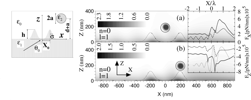
Figure 4: Left figure: Scattering geometry. Insets: Force curves on a silicon cylinder with $a=60$ $nm$ scanned at $d=132.6$ $nm$. (a) Horizontal force. (b) Vertical force. Solid line: $\lambda=638$ $nm$ (on resonance). Broken line: $\lambda=538$ $nm$ (off resonance). Thin solid line in (b): $|H/H_{o}|^{2}$ at $z=d+a$ in absence of particle. Peak value: $|H/H_{o}|^{2}=0.07$. Bottom figures: Spatial distribution $|H/H_{o}|^{2}$ in this configuration. The cylinder center is placed at: $(0,192.6)$ $nm$ (Fig. 4(a)), and at: $(191.4,192.6)$ $nm$ (Fig. 4(b)). The wavelength ($\lambda=638$ $nm$) excites the $(n,l)$ Mie resonance. (From Ref. [Lester 01]).

A silicon cylinder of radius $a=60$ $nm$ in front of a flat dielectric surface with the same value of $\epsilon_{1}$ as considered here, has a Mie resonance excited by the transmitted evanescent wave at $\lambda=638$ $nm$ ($\epsilon_{2}=14.99+i0.14$) [Arias-González 00]. Those eigenmodes are characterized by $n=0$, $l=1$, for $p$ polarization, and $n=1$, $l=1$, for $s$ polarization. We consider the two protrusion interface (Figure 4, left). Insets of Figures 4(a) and 4(b), corresponding to a $p$–polarized incident beam, show the electromagnetic force on the particle as it scans horizontally above the flat surface with two protrusions with parameters $\sigma=63.8$ $nm$, $h=127.6$ $nm$ and $X_{0}=191.4$ $nm$, both at resonant $\lambda$ and out of resonance ($\lambda=538$ $nm$). The particle scans at $d=132.6$ $nm$. Inset (a) shows the force along the $OX$ axis. As seen, the force is positive and, at resonance, it has two remarkable maxima corresponding to the two protrusions, even though they appear slightly shifted due to surface propagation of the evanescent waves transmitted under TIR, which produce the Goos–Hänchen shift of the reflected beam. The vertical force on the particle, on the other hand, is negative, namely attractive, (cf. Inset (b)), and it has two narrow peaks at $x$ just at the position of the protrusions. The signal being again remarkably stronger at resonant illumination. Similar force signal enhancements are observed for $s$–polarization. In this connection, it was recently found that this attractive force on such small dielectric particles monotonically increases as they approach a dielectric flat inteface [Chaumet 00a].

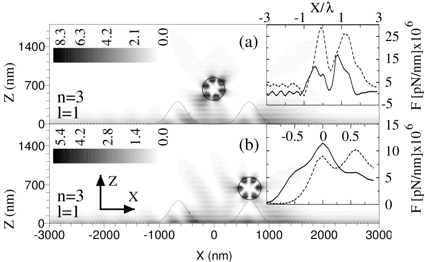
Figure 5: Insets: Force on a silicon cylinder with $a=200$ $nm$ scanned at $d=442$ $nm$. (a) $\lambda=919$ $nm$ (on resonance). (b): $\lambda=759$ $nm$ (off resonance). Solid line: Vertical force. Broken line: Horizontal force. Figures: $|E/E_{o}|^{2}$ in this configuration. The cylinder center is placed at: $(0,642)$ $nm$ (Fig. 5(a)), and at: $(638,642)$ $nm$ (Fig. 5(b)). The wavelength ($\lambda=919$ $nm$) excites the $(n,l)$ Mie resonance. (From Ref. [Lester 01]).

It should be remarked that, by contrast and as expected [Nieto-Vesperinas 91, Greffet 97], the near field–intensity distribution for the magnetic field $H$, normalized to the incident one $H_{0}$, has many more components and interference fringes than the force signal, and thus, the resemblance of its image with the interface topography is worse. This is shown in Inset (b) (thin solid line), where we have plotted this distribution in the absence of particle at $z=d+a$ for the same illumination conditions and parameters as before. This is the one that ideally the particle scan should detect in NSOM.

It is also interesting to investigate the near–field intensity distribution map. Figures 4(a) and 4(b) show this for the magnetic field $H$ in $p$ polarization for resonant illumination, $\lambda=638$ $nm$, at two different positions of the cylinder, which correspond to $x=0$ and $191.4$ $nm$, respectively. We notice, first, the strong field concentration inside the particle, corresponding to the excitation of the $(n=0,l=1)$ –eigenmode. When the particle is over one bump, the variation of the near field intensity is larger in the region closer to it, this being responsible for the stronger force signal on the particle at this position. Similar results are observed for $s$–polarized waves, in this case, the $(n=1,l=1)$–eigenmode of the cylinder is excited and one can appreciate remarkable fringes along the whole interface due to interference of the surface wave, transmitted under TIR, with scattered waves from both the protrusions and the cylinder.

An increase of the particle size yields stronger force signals at the expense of losing some resolution. Figures 5(a) and 5(b) show the near electric field intensity distribution for $s$ polarization at two different positions of a cylinder with radius $a=200$ $nm$, the parameters of the topography now being $\sigma=212.7$ $nm$, $h=425.3$ $nm$ and $X_{0}=\pm 638$ $nm$. The distance is $d=442$ $nm$. The resonant wavelength is now $\lambda=919$ $nm$ ($\epsilon_{2}=13.90+i0.07$). Insets of Figures 5(a) and  5(b) illustrate the force distribution as the cylinder moves along $OX$. The force peaks, when the resonant wavelength is considered, are positive, because now, the scattering force on this particle of larger scattering cross section is greater than the gradient force. They also appear shifted with respect to the protrusion positions, once again due to surface travelling waves under TIR. There are weaker peaks, or absence of them at non–resonant $\lambda$. Similar results occur for a $p$–polarized beam at the resonant wavelength $\lambda=759$ $nm$ ($\epsilon_{2}=13.47+i0.04$). For both polarizations the $(n=3,l=1)$ Mie eigenmode of the cylinder is now excited. The field distribution is well–localized inside the particle and it has the characteristic standing wave structure resulting from interference between counterpropagating whispering–gallery modes circumnavegating the cylinder surface. It is remarkable that this structure appears as produced by the excitation of propagating waves incident on the particle [Arias-González 00], these being due to the coupling of the incident and the TIR surface waves with radiating components of the transmitted field, which are created from scattering with the interface protrusions. Although not shown here, we should remark that illumination at non–resonant wavelengths do not produce such a field concentration within the particle, then the field is extended throughout the space, with maxima attached to the flat portions of the interface (evanescent wave) and along certain directions departing from the protrusions (radiating waves from scattering at these surface defects).

Evanescent components of the electromagnetic field and multiple scattering among several objects are often difficult to handle in an experiment. However, there are many physical situations that involve these phenomena. In this section we have seen that the use of the field inhomogeneity, combined with (and produced by) morphology–dependent resonances and multiple scattering, permit to imaging a surface with defects. Whispering–gallery modes in dielectric particles, on the other hand, produce also evanescent fields on the particle surface which enhance the strength of the force signal. The next section is aimed to study metallic particles under the same situation as previously discussed, exciting now plasmon resonances on the objects.

5.3 Distributions of Forces on Metallic Particles
Over Corrugated Surfaces Illuminated Under TIR

Dielectric particles suffer intensity gradient forces under light illumination due to radiation pressure, which permit one to hold and manipulate them by means of optical tweezers [Ashkin 77] in a variety of applications such as spectroscopy [Sasaki 91, Misawa 92, Misawa 91], phase transitions in polymers [Hotta 98], and light force microscopy of cells [Pralle 99, Pralle 98] and biomolecules [Smith 96]. Metallic particles, however, were initially reported to suffer repulsive electromagnetic scattering forces due to their higher cross sections [Ashkin 92], although later [Svoboda 94] it was shown that nanometric metallic particles (with diameters smaller than $50$ $nm$) can be held in the focal region of a laser beam. Further, it was demonstrated in an experiment [Sasaki 00] that metallic particles illuminated by an evanescent wave created under TIR at a substrate, experience a vertical attractive force towards the plate, while they are pushed horizontally in the direction of propagation of the evanescent wave along the surface. Forces in the $fN$ range were measured.

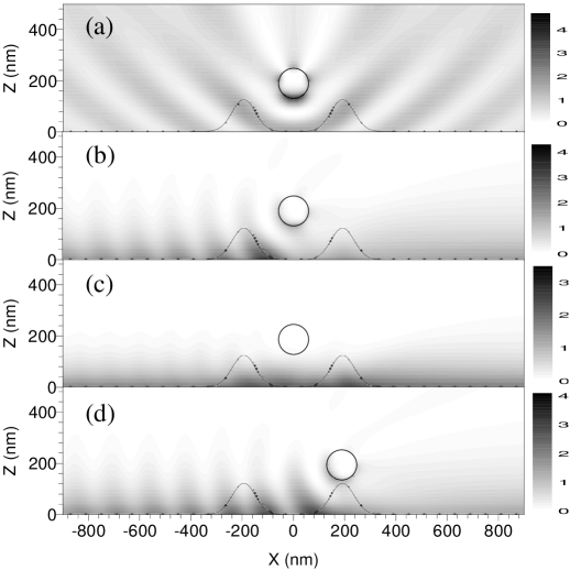
Figure 6: $|H/H_{o}|^{2}$, $P$ polarization, from a silver cylinder with $a=60$ $nm$ immersed in water, on a glass surface with defect parameters $X_{0}=\pm 191.4$ $nm$, $h=127.6$ $nm$ and $\sigma=63.8$ $nm$, at distance $d=132.6$ $nm$. Gaussian beam incidence with $W=4000$ $nm$. 6(a): $\lambda=387$ $nm$ (on resonance), $\theta_{o}=0^{o}$. 6(b): $\lambda=387$ $nm$ (on resonance), $\theta_{o}=66^{o}$. 6(c): $\lambda=316$ $nm$ (off resonance), $\theta_{o}=66^{o}$. 6(d): $\lambda=387$ $nm$ (on resonance), $\theta_{o}=66^{o}$. The cylinder center is placed at $(0,192.6)$ nm in 6(a), 6(b) and 6(c), and at $(191.4,192.6)$ nm in 6(d). (From Ref. [Arias-González 01c]).

Plasmon resonances in metallic particles are not so efficiently excited as mor-phology–dependent resonances in non–absorbing high–refractive–index dielectric particles (e.g., see Refs. [Arias-González 01b, Arias-González 00]) under incident evanescent waves. The distance from the particle to the surface must be very small to avoid the evanescent wave decay normal to the propagation direction along the surface. In this section we address the same configuration as before using water as the immersion medium. The critical angle for the glass–water interface is $\theta_{c}=61.28^{o}$. A silver cylinder of radius $a$ at distance $d+a$ from the flat portion of the surface is now studied.

In Figure 6 we plot the near–field intensity distribution $|H/H_{0}|^{2}$ corresponding to the configuration of inset in Figure 4. A silver cylinder of radius $a=60$ $nm$ scans at constant distance $d=162.6$ $nm$ above the interface. The system is illuminated by a $p$–polarized Gaussian beam ($W=4000$ $nm$) at $\theta_{0}=0^{o}$ and $\lambda=387$ $nm$ ($\epsilon_{2}=-3.22+i0.70$). The surface protrusions are positioned at $X_{0}=\pm 191.4$ $nm$ with height $h=127.6$ $nm$ and $\sigma=63.8$ $nm$. Figure 6(a) shows the aforementioned distribution when the particle is centered between the protrusions. The plasmon resonance is excited as manifested by the field enhancement on the cylinder surface, which is higher in its lower portion. At this resonant wavelength, the main Mie coefficient contributor is $n=2$, which can also be deduced from the interference pattern formed along the particle surface: the number of lobes must be $2n$ along this surface [Owen 81]. Figure 6(b) shows the same situation but with $\theta_{0}=66^{o}$. The field intensity close to the particle is higher in Figure 6(a) because in Figure 6(b) the distance $d$ is large enough to obliterate the resonance excitation due to the decay of the evanescent wave created by TIR [Arias-González 01b]. However, the field intensity is markedly different from the one shown in Figure 6(c), in which the wavelength has been changed to $\lambda=316$ $nm$ ($\epsilon_{2}=0.78+i1.07$) so that there is no particle resonance excitation at all. Figure 6(d) shows the same situation as in Figure 6(b) but at a different $X$–position of the particle. In Figure 6(c), the interference in the scattered near–field due to the presence of the particle is rather weak; the field distribution is now seen to be mainly concentrated at low $z$ as an evanescent wave travelling along the interface, and this distribution does not substantially change as the particle moves over the surface at constant $z$. By contrast, in Figures 6(b) and 6(d) the intensity map is strongly perturbed by the presence of the particle. As we shall see, this is the main reason due to which optical force microscopy is possible at resonant conditions with such small metallic particles used as nanoprobes, and not so efficient at non–resonant wavelengths. In connection with these intensity maps (cf. Figures 6(b) and 6(d)), we should point out the interference pattern on the left side of the cylinder between the evanescent wave and the strongly reflected waves from the particle, that in resonant conditions behaves as a strongly radiating antenna [Arias-González 01b, Arias-González 00, Krenn 99]. This can also be envisaged as due to the much larger scattering cross section of the particle on resonance, hence reflecting backwards higher intensity and thus enhancing the interference with the evanescent incident field. The fringe spacing is $\lambda/2$ ($\lambda$ being the corresponding wavelength in water). This is explained as follows: The interference pattern formed by the two evanescent waves travelling on the surface opposite to each other, with the same amplitude and no dephasing, is proportional to $\exp(-2\kappa z)\cos^{2}(n_{1}k_{0}\sin\theta_{0}x)$, with $\kappa=(n_{1}^{2}\sin^{2}\theta_{0}-n_{0}^{2})^{1/2}$. The distance between maxima is $\Delta x=\lambda/(2n_{1}\sin\theta_{0})$. For the angles of incidence used in this work under TIR ($\theta_{0}=66^{0}$ and $72^{0}$), $\sin\theta_{0}\approx 0.9$, and taking into account the refractive indices of water and glass, one can express this distance as $\Delta x\approx\lambda/2n_{0}$. The quantity $\Delta x$ is similar to the fringe period below the particle in Figure 6(a), now attributted to the interference between two opposite travelling plane waves, namely, the one transmitted through the interface and the one reflected back from the particle.

Figure 7: Force on a silver cylinder with $a=60$ $nm$ immersed in water, scanned at constant distance $d=132.6$ $nm$ on a glass surface with defect parameters $X_{0}=\pm 191.4$ $nm$, $h=127.6$ $nm$ and $\sigma=63.8$ $nm$ along $OX$. The incident field is a $p$–polarized Gaussian beam with $W=4000$ $nm$ and $\theta_{0}=66^{o}$. 7(a): Horizontal force. 7(b): Vertical force. Solid curves: $\lambda=387$ $nm$ (on resonance), broken curves: $\lambda=316$ $nm$ (off resonance). Thin lines in 7(b) show $|H/H_{0}|^{2}$ (in arbitrary units), averaged on the perimeter of the cylinder cross section, while it scans the surface. The actual magnitude of the intensity in the resonant case is almost seven times larger than in the non–resonant one. (From Ref. [Arias-González 01c]).

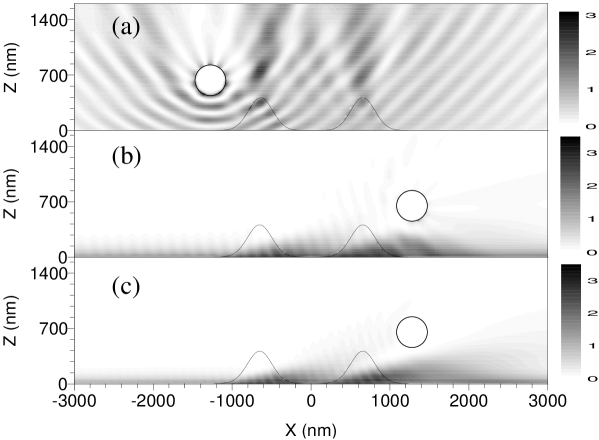
Figure 8: $|H/H_{o}|^{2}$ for $P$ polarization for a silver cylinder with $a=200$ $nm$ immersed in water, on a glass surface with parameters $X_{0}=\pm 638$ $nm$, $h=425.3$ $nm$ and $\sigma=212.7$ $nm$, at distance $d=442$ $nm$. Gaussian beam incidence with $W=4000$ $nm$. 8(a): $\lambda=441$ $nm$ (on resonance), $\theta_{o}=0^{o}$ and the cylinder center placed at $(-1276,642)$ $nm$. 8(b): $\lambda=441$ $nm$ (on resonance), $\theta_{o}=66^{o}$ and the cylinder center placed at $(1276,642)$ $nm$. 8(c): $\lambda=316$ $nm$ (off resonance), $\theta_{o}=66^{o}$ and the cylinder center placed at $(1276,642)$ $nm$. (From Ref. [Arias-González 01c]).

Figure 7 shows the variation of the Cartesian components of the electromagnetic force ($F_{x}$, Fig. 7(a) and $F_{z}$, Fig. 7(d)) on scanning the particle at constant distance $d$ above the interface, at either plasmon resonance excitation ($\lambda=387$ $nm$, solid lines), or off resonance ($\lambda=316$ $nm$, broken lines). The incident beam power (per unit length) on resonance is $3.9320\times 10^{-6}$ $mW/nm$, and $3.9327\times 10^{-6}$ $mW/nm$ at $\lambda=316$ $nm$. The incidence is done with a $p$–polarized Gaussian beam of $W=4000$ $nm$ at $\theta_{0}=66^{o}$. It is seen from these curves that the force distributions resembles the surface topography on resonant conditions with a signal which is remarkably larger than off–resonance. This feature is specially manifested in the $Z$ component of the force, in which the two protrusions are clearly distinguished from the rest of interference ripples, as explained above. Figure 7(b) also shows (thin lines) the scanning that conventional near field microscopy would measure in this configuration, namely, the normalized magnetic near field intensity, averaged on the cylinder cross section. These intensity curves are shown in arbitrary units, and in fact the curve corresponding to plasmon resonant conditions is almost seven times larger than the one off–resonance. The force curves show, on the one hand, that resonant conditions also enhance the contrast of the surface topography image. Thus, the images obtained from the electromagnetic force follows more faithfully the topography than that from the near field intensity. This is a fact also observed with other profiles, including surface–relief gratings. When parameter $h$ is inverted, namely, the interface profile on the left in Fig. 4, then the vertical component of the force distribution presents inverted the contrast. On the whole, one observes from these results that both the positions and sign of the defect height can be distinguished by the optical force scanning.

Figure 9: Force on a silver cylinder with $a=200$ $nm$ immersed in water, scanned at constant distance on a glass surface with parameters $X_{0}=\pm 638$ $nm$, $h=425.3$ and $\sigma=212.7$ $nm$ along $OX$. The incident field is a $p$–polarized Gaussian beam with $W=4000$ $nm$ and $\theta_{0}=66^{o}$. 9(a): Horizontal force. 9(b): Vertical force. Solid curves: $\lambda=441$ $nm$ (on resonance), broken curves: $\lambda=316$ $nm$ (off resonance). Thin solid curves: $\lambda=441$ $nm$ (on resonance) at $\theta_{0}=72^{o}$, thin broken curves: $\lambda=316$ $nm$ (off resonance) at $\theta_{0}=72^{o}$. (From Ref. [Arias-González 01c]).

Figure 8 displays near–field intensity maps for a larger particle ($a=200$ $nm$). Figure 8(a) corresponds to $\theta_{0}=0^{o}$ and a resonant wavelength $\lambda=441$ $nm$ ($\epsilon_{2}=-5.65+i0.75$), with the particle being placed on the left of both protrusions. Figure 8(b) corresponds to $\theta_{0}=66^{o}$ (TIR illumination conditions), at the same resonant wavelength, the particle now being on the right of the protrusions. Figure 8(c) corresponds to $\theta_{0}=66^{o}$ (TIR incidence), at the no resonant wavelength $\lambda=316$ $nm$ ($\epsilon_{2}=0.78+i1.07$), the particle being placed at the right of the protrusions. The incident beam is $p$–polarized with $W=4000$ $nm$. The surface protrusions are positioned at $X_{0}=\pm 638$ $nm$ with height $h=425.3$ $nm$ and $\sigma=212.7$ $nm$. All the relevant size parameters are now comparable to the wavelength, and hence to the decay length of the evanescent wave. That is why now the plasmon resonance cannot be highly excited. When no resonant wavelength is used, the intensity interference fringes due to the presence of the particle are weaker. On the other hand, Figure 8(a) shows the structure of the near–field scattered under $\theta_{0}=0^{o}$. There are three objects that scatter the field: the two protrusions and the particle. They create an inteference pattern with period $\lambda/2$ (with $\lambda$ being the wavelength in water). Besides, the particle shows an inteference pattern around its surface due to the two counterpropagating plasmon waves which circumnavegate it [Arias-González 01b, Arias-González 00]. The number of lobes along the surface is nine, which reflects that the contribution to the field enhancement at this resonant wavelength comes from Mie’s coefficients $n=5$ and $n=4$. Figure 8(b) shows weaker excitation of the same plasmon resonance under TIR conditions. Now, the interference pattern at the incident side of the configuration is also evident. This pattern again has a period $\lambda/2$ ($\lambda$ being the wavelength in water). If non–resonant illumination conditions are used, the particle is too far from the surface to substantially perturb the transmitted evanescent field, then the intensity distribution of this field remains closely attached to the interface, and it is scattered by the surface protrusions. The field felt by the particle in this situation is not sufficient to yield a well–resolved image of the surface topography, as shown next for this same configuration.

Figure 9 shows the components of the force ($F_{x}$, Figure 9(a) and $F_{z}$, Figure 9(b)) for either plasmon excitation conditions ($\lambda=441$ $nm$, solid lines), or off–resonance ($\lambda=316$ $nm$, broken lines), as the cylinder scans at constant distance $d$ above the surface. The incidence is done with a $p$–polarized Gaussian beam of $W=4000$ $nm$ at either $\theta_{0}=66^{o}$ (thick curves) or $\theta_{0}=72^{o}$ (thin curves). The incident beam power (per unit length) is $3.9313\times 10^{-6}$ $mW/nm$ on resonance and $3.9327\times 10^{-6}$ $mW/nm$ at $\lambda=316$ $nm$ when $\theta_{0}=66^{o}$, and $3.9290\times 10^{-6}$ $mW/nm$ on resonance and $3.9315\times 10^{-6}$ $mW/nm$ at $\lambda=316$ $nm$ when $\theta_{0}=72^{o}$. As before, resonant conditions provide a better image of the surface topography making the two protrusions distinguishable with a contrast higher than the one obtained without plasmon excitation. The surface image corresponding to the force distribution is better when the protrusions (not shown here) are inverted because then the particle can be kept closer to the interface. Again, the curve contrast yielded by protrusions and grooves is inverted from each other. The positions of the force distribution peaks corresponding to the protrusions now appear appreciably shifted with respect to the actual protrusions’ position. This shift is explained as due to the Goos–Hänchen effect of the evanescent wave [Lester 01]. We observe that the distance between these peaks in the $F_{z}$ curve is aproximately $2X_{0}$. This shift is more noticeable in the force distribution as the probe size increases. Again, the $F_{z}$ force distribution has a higher contrast at the (shifted) position of the protrusions. The force signal with these bigger particles is larger, but the probe has to be placed farther from the surface at constant height scanning. This affects the strength of the signal. Finally, it is important to state that the angle of incidence (supposed to be larger than the critical angle $\theta_{c}$) influences both the contrast and the strength of the force: the contrast decreases as the angle of incidence increases. At the same time, the strength of the force signal also diminishes.

As seen in the force figures for both sizes of particles, most curves contain tiny ripples. They are due to the field intensity interference pattern as shown in Figures 6 and 8, and discussed above. As the particle moves, the force on it is affected by this interference. As a matter of fact, it can be noted in the force curves that these tiny ripples are mainly present at the left side of the particle, which is the region where stronger interference takes place.

It is worth remarking, however, that these oscillations are less marked in the force distribution (cf. their tiny ripples), than in the near field intensity distribution, where the interference patterns present much higher contrast.

As stated in the previous section, evanescent fields and multiple scattering are fruitful to extracting information from a detection setup. The latter is, at the same time, somewhat troublesome as it cannot be neglected at will. This incovenient is well–known in NSOM, but it is diminished in PFM, as remarked before. The smoother signal provided by the force is underlined by two facts: one is the averaging process on the particle surface, quantitatively interpreted from the field surface integration involved in Maxwell’s stress tensor. Other is the local character of the force acting at each point of the particle surface. Metallic particles are better candidates as probes of PFM in comparison to dielectric particles, since the force signal is not only enhanced at resonance conditions, but it is also bigger and presents better resolution. However, dielectric particles are preferred when the distance to the interface is large, since then the weak evanescent field present at these distances presents better coupling to the whispering–gallery modes than to the plasmon surface waves of metallic particles.

5.4 On the Attractive and Repulsive Nature of
Vertical Forces and Their Orders of Magnitude

The horizontal forces acting on the particle are scattering forces due to radiation pressure of both the incident evanescent wave and the field scattered by the protrusions, thus the forces are positive in all the cases studied. As for the vertical forces, two effects compete in determining their sign. First, is the influence of the polarizability [Chaumet 00b, Chaumet 00a], which depends on the polarization of the illumination. On the other hand, it is well known that an evanescent wave produces only gradient forces in the vertical direction. For silver cylinders, the force at wavelength $\lambda=387$ ($\epsilon_{2}=-3.22+i0.70$) and at $\lambda=441$ $nm$ ($\epsilon_{2}=-5.65+i0.75$) must be attractive, while at $\lambda=316$ $nm$ ($\epsilon_{2}=0.78+i1.07$), the real part of the polarizability changes its sign, and so does the gradient force, thus becoming repulsive (on cylinders of not very large sizes, as here). However, in the cases studied here, not only the multiple scattering of light between the cylinder and the flat portion of the interface, but also the surface defects, produce scattered waves both propagating (into $z>0$) and evanescent under TIR conditions. Thus, the scattering forces also contribute to the $z$–component of the force. This affects the sign of the forces, but it is more significant as the size of the objects increases. In larger cylinders and defects (cf. Figure 9), the gradient force is weaker than the scattering force thus making $F_{z}$ to become repulsive on scanning at $\lambda=441$ $nm$ (plasmon excited). On the other hand, for the smaller silver cylinders studied (cf. Figure 7), the gradient force is greater than the scattering force at $\lambda=387$ $nm$ (plasmon excited), and thus the force is attractive in this scanning. Also, as the distance between the particle and the surface decreases, the gradient force becomes more attractive [Chaumet 00b, Chaumet 00a]. This explains the dips and change of contrast in the vertical force distribution on scanning both protrusions and grooves. At $\lambda=316$ $nm$ (no plasmon excited), both scattering and gradient forces act cooperatively in the vertical direction making the force repulsive, no matter the size of the cylinder. For the silicon cylinder, as shown, the vertical forces acting under TIR conditions are attractive in absence of surface interaction (for both polarizations and the wavelengths used). However, this interaction is able to turn into repulsive the vertical force for $S$ polarization at $\lambda=538$ $nm$, due to the scattering force.

This study also reveals the dependence of the attractive or repulsive nature of the forces on the size of the objects (probe and defects of the surface), apart from the polarizability of the probe and the distance to the interface, when illumination under total internal reflection is considered. The competition between the strength of the scattering and the gradient force determines this nature.

The order of magnitude of the forces obtained in the preceding 2D calculations is consistent with that of forces in experiments and 3D calculations of Refs. [Pohl 93, Güntherodt 95, Depasse 92, Sugiura 93, Kawata 92, Dereux 94, Girard 94, Almaas 95, Novotny 97, Hecht 96, Okamoto 99, Chaumet 00b] and [Chaumet 00a]. Suppose a truncated cylinder with axial length $L=10$ $\mu m$, and a Gaussian beam with $2W\sim 10$ $\mu m$. Then, a rectangular section of $L\times 2W=10^{2}$ $\mu m^{2}$ is illuminated on the interface. For an incident power $P_{0}\sim 1$ $mW$, spread over this rectangular section, the incident intensity is $I_{0}\sim 10^{-2}$ $mW/\mu m^{2}$, and the force range from our calculations is $F\sim 10^{-2}-10^{-1}$ $pN$. Thus, the forces obtained in Figures 9(b) and 9(d) are consistent with those presented, for example, in Ref. [Kawata 92].

6 Concluding Remarks & Future Prospects

The forces exerted by both propagating and evanescent fields on small particles are the basis to understand estructural characteristics of time–harmonic fields. The simplest evanescent field that can be built is the one that we have illustrated on transmission at a dielectric interface when TIR conditions occur. Both dielectric and metallic particles are pushed along the direction of propagation of the evanescent field, independently of the size (scattering and absorption forces). By contrast, forces behave differently along the decay direction (gradient forces) on either dielectric and metallic particles, as studied for dipolar–sized particles, Section 2. The analysis done in presence of a rough interface, and with particles able to interact with it show that scattering, absorption and gradient forces act both in the amplitude and phase directions, when multiple scattering takes place. Moreover, the excitation of particle resonances enhances this interaction, and, at the same time, generates evanescent fields (surface waves) on their surface, which makes even more complex this mixing among force components. Thus, an analysis based on a small particle isolated is not feasible due to the high inhomogeneity of the field.

It is, however, this inhomogeneity what provides a way to imaging a surface with structural features, such as topography. The possibility offered by the combination of evanescent fields and Mie resonances is however not unique. As inhomgeneous fields (which can be analitically decomposed into propagating and evanescent fields [Nieto-Vesperinas 91]) play an important role in the mechanical action of the electromagnetic wave on dielectric particles (either on or out of resonance), they can be used to operate at the nanometric scale on such entities, to assist the formation of ordered particle structures as for example [Burns 89, Burns 90, Antonoyiannakis 97, Antonoyiannakis 97, Malley 98, Bayer98, Barnes 02], with help of these resonances. Forces created by evanescent fields on particles and morphology–dependent resonances are the keys to control the optical binding and the formation of photonic molecules. Also, when a particle is used as a nanodetector, these forces are the signal in a scheme of photonic force microscopy as modeled in this article. It has been shown that the evanescent field forces and plasmon resonance excitations permit to manipulate metallic particles [Novotny 97, Chaumet 01, Chaumet 02], as well as to make such microscopy [Arias-González 01c]. Nevertheless, controlled experiments on force magnitudes, both due to evanescent and propagating waves, are yet scarce and thus desirable to be fostered.

The concepts released in this article open an ample window to investigate on soft matter components like in cells and molecules in biology. Most folding processes require small forces to detect and control in order not to alter them and be capable of actuating and extracting information from them.

General Annotated References

Complementary information and sources for some of the contents treated in this report can be found in next bibliography:

• Electromagnetic optics: there are many books where to find the basis of the electromagnetic theory and optics. We cite here the most common: [Jackson 75, Born 99c]. The Maxwell’s Stress Tensor is analysed in [Jackson 75, Stratton 41]. The mathematical level of these textbooks is similar to the one in this report.

• Mie theory can be found in [van de Hulst 81, Kerker 69, Bohren 83]. In these textbooks, Optics of particles is develop with little mathematics and all of them are comparable in contents.

• Resonances can be understood from the textbooks before, but a more detailed information, with applications and the implications in many topics can be found in the following references: [Arias-González 02c, Hill 88, Barber 90]. The last two references are preferently centred in dielectric particles. The first one compiles some of the information in these two references and some other from scientific papers. Surface plasmons, on the other hand, are studied in depth in [Raether 88]. They are easy to understand from general physics.

• Integral equations in scattering theory and angular spectrum representation (for the decomposition of time–harmonic fields in propagating and evanescent components) are treated in [Nieto-Vesperinas 91]. The mathematical level is similar to the one in this report.

• The Coupled Dipole Method can be found in the scientific papers cited in Section 4.1. A More didactical reference is [Chaumet 98, Rahmani 00]. The information shed in this report on the CDM is extended in these references.

• The dipolar approximation, in the context of optical forces and evanescent fields, can be complemented in scientific papers: [Gordon 73, Chaumet 00c, Arias-González 02b] and in the monograph: [Novotny 00].

• A more detailed discussion on the sign of optical forces for dipolar particles, as well as larger elongated particles, can be found in the scientific papers [Arias-González 02a, Arias-González 02b, Chaumet 00b].

• Monographs on NSOM and tweezers: [Nieto-Vesperinas 96, Sheetz 97].

Acknowledgments

We thank P. C. Chaumet and M. Lester for work that we have shared through the years. Grants from DGICYT and European Union, as well as a fellowship of J. R. Arias-González from Comunidad de Madrid, are also acknowledged.

References

- [Agarwal 75a] G. S. Agarwal. Quantum electrodynamics in the presence of dielectrics and conductors. I. Electromagnetic–field response functions and black–body fluctuations in finite geometries. Phys. Rev. A, 11, pages 230–242, 1975.
- [Agarwal 75b] G. S. Agarwal. Quantum electrodynamics in the presence of dielectrics and conductors. IV. General theory for spontaneous emission in finite geometries. Phys. Rev. A, 12, pages 1475–1497, 1975.
- [Allegrini 01] M. Allegrini, N. García and O. Marti, editors. Nanometer scale science and technology, Amsterdam, 2001. Società Italiana di Fisica, IOS PRESS. in Proc. Int. Sch. E. Fermi, Varenna.
- [Almaas 95] E. Almaas and I. Brevik. Radiation forces on a micrometer–sized sphere in an evanescent field. J. Opt. Soc. Am. B, 12, pages 2429–2438, 1995.
- [Alonso 68] M. Alonso and E. J. Finn. Quantum and Statistical Physics. Addison–Wesley Series in Physics, Addison–Wesley, Reading, MA, 1968.
- [Antonoyiannakis 97] M. I. Antonoyiannakis and J. B. Pendry. Mie resonances and bonding in photonic crystals. Europhys. Lett., 40, pages 613–618, 1997.
- [Antonoyiannakis 97] M. I. Antonoyiannakis and J. B. Pendry. Electromagnetic forces in photonic crystals. Phys. Rev. B, 60, pages 2363–2374, 1999.
- [Arias-González 99] J. R. Arias-González, M. Nieto-Vesperinas and A. Madrazo. Morphology–dependent resonances in the scattering of electromagnetic waves from an object buried beneath a plane or a random rough surface. J. Opt. Soc. Am. A, 16, pages 2928–2934, 1999.
- [Arias-González 00] J. R. Arias-González and M. Nieto-Vesperinas. Near field distributions of resonant modes in small dielectric objects on flat surfaces. Opt. Lett., 25, pages 782–784, 2000.
- [Arias-González 01a] J. R. Arias-González, P. C. Chaumet and M. Nieto-Vesperinas. Nanoparticles on surfaces: resonances and optical forces. In Nanometer Scale Science and Technology, 2001. [Allegrini 01].
- [Arias-González 01b] J. R. Arias-González and M. Nieto-Vesperinas. Resonant near–field eigenmodes of nanocylinders on flat surfaces under both homogeneous and inhomogeneous lightwave excitation. J. Opt. Soc. Am. A, 18, pages 657–665, 2001.
- [Arias-González 01c] J. R. Arias-González, M. Nieto-Vesperinas and M. Lester. Modeling photonic–force microscopy with metallic particles under plasmon eigenmode excitation. Phys. Rev. B, 65, page 115402, 2002.
- [Arias-González 02a] J. R. Arias-González and M. Nieto-Vesperinas. Radiation pressure over dielectric and metallic nanocylinders on surfaces: polarization dependence and plasmon resonance conditions. Opt. Lett., submitted, 2002.
- [Arias-González 02b] J. R. Arias-González and M. Nieto-Vesperinas. Optical forces on small particles: attractive and repulsive forces and plasmon resonance conditions. J. Opt. Soc. Am. A, submitted, 2002.
- [Arias-González 02c] J. R. Arias-González Electromagnetic resonances in light scattering by surfaces and objects: Detection and characterization of hidden objects, Near field and Optical forces. Universidad Complutense de Madrid, Spain, 2002.
- [Ashkin 77] A. Ashkin and J. M. Dziedzic. Observation of Resonances in the Radiation Pressure on Dielectric Spheres. Phys. Rev. Lett., 38, pages 1351–1354, 1977.
- [Ashkin 86] A. Ashkin, J. M. Dziedzic, J. E. Bjorkholm and S. Chu. Observation of a single–beam gradient force optical trap for dielectric particles. Opt. Lett., 11, pages 288–290, 1986.
- [Ashkin 92] A. Ashkin and J. M. Dziedzic. Conditions for conductance quantization in realistic models of atomic–scale metallic contacts. Appl. Phys. Lett., 24, pages 586–589, 1992.
- [Baños 66a] A. Baños. 1966. in [Baños 66b], chapter 2.
- [Baños 66b] A. Baños. Dipole Radiation in the Presence of a Cunducting Half–Space. Pergamon Press, Oxford, 1966.
- [Barber 82] P. W. Barber, J. F. Owen and R. K. Chang. Resonant Scattering for Characterization of Axisymmetric Dielectric Objects. IEEE Trans. Antennas Propagat., 30, pages 168–172, 1982.
- [Barber 88] P. W. Barber and R. K. Chang, editors. Optical Effects Associated With Small Particles. World Scientific, Singapore, 1988.
- [Barber 90] P. W. Barber and S. C. Hill. Light Scattering by Particles: Computational Methods. World Scientific, Singapore, 1990.
- [Barnes 02] M. D. Barnes, S. M. Mahurin, A. Mehta, B. G. Sumpter and D. W. Noid. Three-Dimensional Photonic “Molecules” from Sequentially Attached Polymer-Blend Microparticles. Phys. Rev. Lett., 88, page 015508, 2002.
- [Bayer98] M. Bayer, T. Gutbrod, J. P. Reithmaier, A. Forchel, T. L. Reinecke, P. A. Knipp, A. A. Dremin and V. D. Kulakovskii. Optical Modes in Photonic Molecules. Phys. Rev. Lett., 81, pages 2582–2585 , 1998.
- [Benincasa 87] D.S. Benincasa, P.W. Barber, J-Z. Zhang, W-F. Hsieh and R.K. Chang. Spatial distribution of the internal and near–field intensities of large cylindrical and spherical scatterers. Appl. Opt., 26, pages 1348–1356, 1987.
- [Bohren 83] C. F. Bohren and D. R. Huffman. Absortion and Scattering of Light by Small Particles. Wiley–Interscience Publication, New York, 1983.
- [Born 99a] M. Born and E. Wolf. 1999. in [Born 99c], section 11.4.2.
- [Born 99b] M. Born and E. Wolf. 1999. in [Born 99c], pp 34.
- [Born 99c] M. Born and E. Wolf. Principles of optics. Cambridge University Press, Cambridge, 7nd edition, 1999.
- [Bryant 66] H. C. Bryant and A. J. Cox. Mie Theory and the Glory. J. Opt. Soc. Am. A, 56, pages 1529–1532, 1966.
- [Burns 90] M. M. Burns, J.-M. Fournier and J. A. Golovchenco. Optical Matter: Crystallization and Binding in Intense Optical Fields. Science, 249, pages 749–754, 1990.
- [Burns 89] M. M. Burns, J.-M. Fournier and J. A. Golovchenco. Optical binding. Phys. Rev. Lett., 63, pages 1233-1236, 1989.
- [Chang 94] S. Chang, J. H. Jo and S. S. Lee. Theoretical calculations of optical force exerted on a dielectric sphere in the evanescent field generated with a totally–reflected focused gaussian beam. Opt. Commun., 108, pages 133–143, 1994.
- [Chaumet 00a] P. C. Chaumet and M. Nieto-Vesperinas. Coupled dipole method determination of the electromagnetic force on a particle over a flat dielectric substrate. Phys. Rev. B, 61, pages 14119–14127, 2000.
- [Chaumet 00b] P. C. Chaumet and M. Nieto-Vesperinas. Electromagnetic force on a metallic particle in presence of a dielectric surface. Phys. Rev. B, 62, pages 11185–11191, 2000.
- [Chaumet 00c] P. C. Chaumet and M. Nieto-Vesperinas. Time–averaged total force on a dipolar sphere in an electromagnetic field. Opt. Lett., 25, pages 1065–1067, 2000.
- [Chaumet 01] P. C. Chaumet and M. Nieto-Vesperinas. Optical binding of particles with or without the presence of a flat dielectric surface. Phys. Rev. B, 64, page 035422, 2001.
- [Chaumet 02] P. C. Chaumet, A. Rahmani and M. Nieto-Vesperinas. Optical Trapping and Manipulation of Nano-objects with an Apertureles Probe. Phys. Rev. Lett., 88, page 123601, 2002.
- [Chaumet 98] P. C. Chaumet. Diffusion d’une Onde Electromagnétique par des Structures Arbitraires: Application à la Emission de Lumière en STM. Université de Bourgogne, France, 1998.
- [Chew 79] H. W. Chew, D.-S. Wang and M. Kerker. Elastic scattering of evanescent electromagnetic waves (T). Appl. Opt., 18, 2679, 1979.
- [Clapp 99] A. R. Clapp, A. G. Ruta and R. B. Dickinson. Three–dimensional optical trapping and evanescent wave light scattering for direct measurement of long range forces between a colloidal particle and a surface. Rev. Sci. Instr., 70, pages 2627–2636, 1999.
- [Collot 93] L. Collot, V. Lefèvre-Seguin, M. Brune, J.M. Raimond and S. Haroche. Very High– Whispering–Gallery Mode Resonances Observed on Fused Silica Microspheres. Europhys. Lett., 23, pages 327–334, 1993.
- [Crocker 94] J. C. Crocker and D. G. Grier. Microscopic measurement of the pair interaction potential of charge–stabilized colloid. Phys. Rev. Lett., 73, pages 352–355, 1994.
- [Depasse 92] F. Depasse and D. Courjon. Opt. Commun., 87, 79, 1992.
- [Dereux 94] A. Dereux, C. Girard, O. J. F. Martin and M. Devel. Movement of micrometer–sized particles in the evanescent field of a laser beam. Europhys. Lett., 26, pages 37–42, 1994.
- [Dogariu 00] A. C. Dogariu and R. Rajagopalan. Optical Traps as Force Transducers: The effects of Focusing the Trapping Beam through a Dielectric Interface. Langmuir, 16, pages 2770–2778, 2000.
- [Draine 88] B. T. Draine. The Discrete–dipole approximation and its application to interstellar graphite grains. Astrophys. J., 333, pages 848–872, 1988.
- [Dungey 91] C. E. Dungey and C. F. Bohren. Light scattering by nonspherical particles: a refinement to the coupled–diple method. J. Opt. Soc. Am. A, 8, pages 81–87, 1991.
- [Fahlen 68] T. S. Fahlen and H. C. Bryant. Optical Back Scattering from Single Water Droplets. J. Opt. Soc. Am., 58, pages 304–310, 1968.
- [Florin 96] E.-L. Florin, J. K. H. Hörber and E. H. K. Stelzer. High–resolution axial and lateral position sensing using two–photon excitation of fluorophores by a continuous Nd:YAG laser. Appl. Phys. Lett., 69, pages 446–448, 1996.
- [Ghislain 93] L. P. Ghislain and W. W. Webb. Scanning–force microscope based on an optical trap. Opt. Lett., 18, pages 1678–1680, 1993.
- [Girard 94] C. Girard, A. Dereux and O. J. F. Martin. Theoretical analysis of light–inductive forces in scanning probe microscopy. Phys. Rev. B, 49, pages 13872–13881, 1994.
- [Gordon 73] J. P. Gordon. Radiation Forces and Momenta in Dielectric Media. Phys. Rev. A, 8, pages 14–21, 1973.
- [Greffet 97] J. J. Greffet and R. Carminati. Image Formation in Near–field Optics. Prog. Surf. Sci., 56, pages 133–235, 1997.
- [Güntherodt 95] H.-J. Güntherodt, D. Anselmetti and E. Meyer, editors. Forces in scanning probe methods, Dordrecht, 1995. NATO ASI Series, Kluwer Academic Publishing.
- [Hecht 96] B. Hecht, H. Bielefeldt, L. Novotny, Y. Inouye and D. W. Pohl. Local Excitation, Scattering, and Interference of Surface Plasmons. Phys. Rev. Lett., 77, pages 1889–1892, 1996.
- [Hill 88] S. C. Hill and R. E. Benner. Morphology–dependent resonances, chapitre 1. World Scientific, 1988. [Barber 88].
- [Hörber 01] J. K. H. Hörber. Local Probe Techniques in Biology. In Nanometer Scale Science and Technology, 2001. [Allegrini 01].
- [Hotta 98] J. Hotta, K. Sasaki, H. Masuhara and Y. Morishima. Laser–controlled assembling of repulsive unimolecular micelles in aqueous solution. J. Phys. Chem. B, 102, pages 7687–7690, 1998.
- [Jackson 75] J. D. Jackson. Classical Electrodynamics. Wiley–Interscience Publication, New York, 2nd edition, 1975.
- [Kawata 92] S. Kawata and T. Sugiura. Movement of micrometer–sized particles in the evanescent field of a laser beam. Opt. Lett., 17, pages 772–774, 1992.
- [Kawata 96] S. Kawata and T. Tani. Optically driven Mie particles in an evanescent field along a channeled waveguide. Opt. Lett., 21, pages 1768–1770, 1996.
- [Kawata 00] S. Kawata, editor. Near-field Optics and Surface Plasmon Polaritons, Topics in Applied Physics, Springer–Verlag, Berlin, 2000.
- [Keller 93] O. Keller, M. Xiao and S. Bozhevolnyi. Configurational Resonances in Optical Near–Field Microscopy: A Rigorous Point–Dipole Approach. Surf. Sci., 280, pages 217–230, 1993.
- [Kerker 69] M. Kerker. The Scattering of Light and Other Electromagnetic Radiation. Academic Press, New York, 1969.
- [Khare 68] V. Khare and H. M. Nussenzveig. Theory of the Glory. Phys. Rev. Lett., 38, pages 1279–1282, 1968.
- [Klar 88] T. Klar, M. Perner, S. Grosse, G.V. Plessen, W. Spirkl and J. Feldmann. Surface Plasmon resonances in single metallic nanoparticles. Phys. Rev. Lett., 80, pages 4249–4252, 1988.
- [Knight 95] J.C. Knight, N. Dubreuil, V. Sandoghdar, J. Hare, V. Lefèvre-Seguin, J.M. Raimond and S. Haroche. Mapping whispering–gallery modes in microspheres with a near–field probe. Opt. Lett., 20, pages 1515–1517, 1995.
- [Krenn 99] J. R. Krenn, A. Dereux, J. C. Weeber, E. Bourillot, Y. Lacroute, J. P. Goudonnet, G. Schider, W. Gotschy, A. Leitner, F. R. Aussenegg and C. Girard. Squeezing the Optical Near–Field Zone by Plasmon Coupling of Metallic Nanoparticles. Phys. Rev. Lett., 82, pages 2590–2593, 1999.
- [Lester 99] M. Lester and M. Nieto-Vesperinas. Optical forces on microparticles in an evanescent laser field. Opt. Lett., 24, pages 936–938, 1999.
- [Lester 01] M. Lester, J. R. Arias-González and M. Nieto-Vesperinas. Fundamentals and model of photonic–force microscopy. Opt. Lett., 26, pages 707–709, 2001.
- [Malley 98] L. E. Malley, D. A. Pommet and M. A. Fiddy. Optically induced ordering in microparticle suspensions. J. Opt. Soc. Am. B, 15, pages 1590–1595, 1998.
- [Mandel 95] L. Mandel and E. Wolf. Optical Coherence and Quantum Optics. Cambridge University Press, Cambridge, 1995.
- [Misawa 91] H. Misawa, M. Koshioka, K. Sasaki, N. Kitamura and H. Masuhara. Three–dimensional optical trapping and laser ablation of a single polymer latex particle in water. J. Appl. Phys., 70, pages 3829–3836, 1991.
- [Misawa 92] H. Misawa, K. Sasaki, M. Koshioka, N. Kitamura and H. Masuhara. Multibeam laser manipulation and fixation of microparticles. Appl. Phys. Lett., 60, pages 310–312, 1992.
- [Morse 53] P. M. Morse and H. Feshbach. Methods of theoretical physics. McGraw–Hill, New York, 1953.
- [Nieto-Vesperinas 91] M. Nieto-Vesperinas. Scattering and Diffraction in Physical Optics. John Wiley & Sons, Inc, New York, 1991.
- [Nieto-Vesperinas 96] M. Nieto-Vesperinas and N. García, editors. Optics at the nanometer scale, Dordrecht, 1996. NATO ASI Series, Kluwer Academic Publishing.
- [Novotny 97] L. Novotny, R. X. Bian and X. S. Xie. Theory of Nanometric Optical Tweezers. Phys. Rev. Lett., 79, pages 645–648, 1997.
- [Novotny 00] L. Novotny. Forces in Optical Near–fields. In Near-field Optics and Surface Plasmon Polaritons, Topics in Applied Physics, 81, pages 123–141, 2000. [Kawata 00].
- [Okamoto 99] K. Okamoto and S. Kawata. Radiation Force Exerted on Subwavelength Particles near a Nanoaperture. Phys. Rev. Lett., 83, pages 4534–4537, 1999.
- [Owen 81] J. F. Owen, R. K. Chang and P. W. Barber. Internal electric field distributions of a dielectric cylinder at resonance wavelengths. Opt. Lett., 6, pages 540–542, 1981.
- [Paesler 96] M. A. Paesler and P. J. Moyer. Near–Field Optics. John Wiley & Sons, Inc, New York, 1996.
- [Pattanayak 76a] D. N. Pattanayak and E. Wolf. Resonance states as solutions of the Schrödinger equation with a nonlocal boundary condition. Phys. Rev. E, 13, pages 2287–2290, 1976.
- [Pattanayak 76b] D. N. Pattanayak and E. Wolf. Scattering states and bound states as solutions of the Schrödinger equation with nonlocal boundary conditions. Phys. Rev. E, 13, pages 913–923, 1976.
- [Pohl 93] D. W. Pohl and D. Courjon, editors. Near field optics, Dordrecht, 1993. NATO ASI Series, Kluwer Academic Publishing.
- [Pralle 98] A. Pralle, E.-L. Florin, E. H. K. Stelzer and J. K. H. Hörber. Local viscosity probed by photonic force microscopy. Appl. Phys. A, 66, pages S71–S73, 1998.
- [Pralle 99] A. Pralle, M. Prummer, E.-L. Florin, E. H. K. Stelzer and J. K. H. Hörber. Three–dimensional high–resolution particle tracking for Optical tweezers by forward scattered light. Microsc. Res. Tech., 44, pages 378–386, 1999.
- [Prieve 93] D. C. Prieve and J. Y. Walz. Scattering of an evanescent surface wave by a microscopic dielectric sphere . Appl. Opt.-LP, 32, 1629, 1993.
- [Purcell73] E. M. Purcell and C. R. Pennypacker. Scattering and absorption of light by nonspherical dielectric grains. Astrophys. J., 186, pages 705–714, 1973.
- [Raether 88] H. Raether. Surface Plasmons. Springer–Verlag, Berlin Heidelberg, 1988.
- [Rahmani 00] A. Rahmani and F. de Fornel. Emission photonique en espace confiné. Eyrolles and France Télécom-CNET, Paris, 2000.
- [Sasaki 91] K. Sasaki, M. Koshioka, H. Misawa, N. Kitamura and H. Masuhara. Pattern formation and flow control of fine particles by laser–scanning micromanipulation. Opt. Lett., 16, pages 1463–1465, 1991.
- [Sasaki 97] K. Sasaki, M. Tsukima and H. Masuhara. Three–dimensional potential analysis of radiation pressure exerted on a single microparticle. Appl. Phys. Lett., 71, pages 37–39, 1997.
- [Sasaki 00] K. Sasaki, J. Hotta, K. Wada and H. Masuhara. Analysis of radiation pressure exerted on a metallic particle within an evanescent field. Opt. Lett., 25, pages 1385–1387, 2000.
- [Sheetz 97] M. P. Sheetz, editor. Laser Tweezers in Cell Biology. Academic Press, San Diego, CA, 1997.
- [Smith 96] S. B. Smith, Y. Cui and C. Bustamante. Overstretching B–DNA: the elastic response of individual double–stranded and single–stranded DNA molecules. Science, 271, pages 795–799, 1996.
- [Stout 97] A. L. Stout and W. W. Webb. Optical Force Microscopy. Methods Cell Biol., 55, 99, 1997. in [Sheetz 97].
- [Stratton 41] J. A. Stratton. Electromagnetic theory. McGraw–Hill, New York, 1941.
- [Sugiura 93] T. Sugiura and S. Kawata. Photon–pressure exertion on thin film and small particles in the evanescent field. Bioimaging, 1, pages 1–5, 1993.
- [Svoboda 94] K. Svoboda and S. M. Block. Optical trapping of metallic Rayleigh particles. Opt. Lett., 19, pages 13–15, 1994.
- [Tamir 72a] T. Tamir. Inhomogeneous Wave Types at Planar Structures: I. The Lateral Wave. Optik, 36, pages 209–232, 1972.
- [Tamir 72b] T. Tamir. Inhomogeneous Wave Types at Planar Structures: II. Surface Waves. Optik, 37, pages 204–228, 1972.
- [van de Hulst 81] H. C. van de Hulst. Light Scattering by Small Particles. Dover, New York, 1981.
- [Vilfan 98] M. Vilfan, I. Musěvič and M. Č opič. AFM observation of force on a dielectric sphere in the evanescent field of totally reflected light. Europhys. Lett., 43, pages 41–46, 1998.
- [Wada 00] K. Wada, K. Sasaki and H. Masuhara. Optical measurement of interaction potentials between a single microparticle and an evanescent field. Appl. Phys. Lett., 76, pages 2815–2817, 2000.
- [Walz 99] J. Y. Walz. Ray optics calculation of the radiation forces exerted on a dielectric sphere in an evanescent field. Appl. Opt., 38, pages 5319–5330, 1999.
- [Weiss 95] D. S. Weiss, V. Sandoghdar, J. Hare, V. Lefè vre-Seguin, J.M. Raimond and S. Haroche. Splitting of high– Mie modes induced by light backscattering in silica microspheres. Opt. Lett., 20, pages 1835–1837, 1995.
- [Yaghjian 80] A. D. Yaghjian. Electric Dyadic Green’s Functions in the Source Region. Proc. IEEE, 68, pages 248–263, 1980.