Stroboscopic observation of quantum many-body dynamics

Abstract

Recent experiments have demonstrated single-site resolved observation of cold atoms in optical lattices. Thus, in the future it may be possible to take repeated snapshots of an interacting quantum many-body system during the course of its evolution. Here we address the impact of the resulting quantum (anti-)Zeno physics on the many-body dynamics. We use the time-dependent density-matrix renormalization group to obtain the time evolution of the full wave function, which is then periodically projected in order to simulate realizations of stroboscopic measurements. For the example of a one-dimensional lattice of spinless fermions with nearest-neighbor interactions, we find regimes for which many-particle configurations are stabilized or destabilized, depending on the interaction strength and the time between observations.

Introduction. In the last few years ultracold atoms in optical lattices have proven to be a versatile tool for studying various quantum many-body phenomena (Bloch et al., 2008; Lewenstein et al., 2007). Recently, tremendous progress has been achieved by implementing single-site resolved detection (Bakr et al., 2009; Sherson et al., 2010) and addressing (Weitenberg et al., 2011) of atoms. Taken to the next, dynamic level, one may envision observing the evolution of nonequilibrium quantum many-body states via periodic snapshots revealing the position of each single atom. For simpler systems, the effect of frequent observations on the decay of an unstable state (or on the dynamics of a driven transition) has already been discussed and observed, leading to the notion of the quantum (anti-)Zeno effect (Misra and Sudarshan, 1977; Itano et al., 1990; Fischer et al., 2001; Facchi and Pascazio, 2008). Zeno physics has also been seen in cold-atom experiments with atomic loss channels (Syassen et al., 2008) and was theoretically addressed in (García-Ripoll et al., 2009; Daley et al., 2009; Schützhold and Gnanapragasam, 2010; Shchesnovich and Konotop, 2010). Experiments with single-site detection, however, would reveal the effect of observations on the dynamics of a truly interacting quantum many-body system. Here we exploit a numerically efficient approach to simulating the repeated observation of many-particle configurations in interacting lattice models. This represents an idealized version of the dynamics that may be realized in future experiments. We elaborate the main features of this “stroboscopic” many-body dynamics in the case of a one-dimensional (1D) lattice of spin-polarized fermions with nearest-neighbor interactions. We find a variant of the quantum Zeno effect and discuss its tendency to inhibit or accelerate the break-up of certain many-particle configurations. In particular, the decay rate of these configurations depends in a nonmonotonous fashion on the time interval between observations. Later, we show that a similar behavior is expected for the Fermi-Hubbard and Bose-Hubbard model. The discussed features may be seen, e. g., in the expansion of interacting atomic clouds in a lattice.

Model. In this paper, we study spin-polarized fermions in a 1D lattice governed by the Hamiltonian

$$\hat{\mathcal{H}}=-J\sum_{i}\big{(}\hat{c}_{i}^{\dagger}\hat{c}_{i+1}+\mbox{H.c.}\big{)}+V\sum_{i}\hat{n}_{i}\hat{n}_{i+1}\,.$$ (1)

The first term describes hopping with amplitude $J$ between adjacent sites, the second encodes the interaction between fermions at neighboring sites, with $\hat{n}_{i}=\hat{c}_{i}^{\dagger}\hat{c}_{i}$. The Hamiltonian displays a dynamical $V\mapsto-V$ symmetry which shows up in expansion experiments (Schneider et al., ). Following analogous steps as in (Schneider et al., ), we can conclude that if both the initial state and the experimentally measured quantity $\hat{\mathcal{O}}$ are invariant under both time reversal and $\pi$–boost (a translation of all momenta by $\pi$), the observed time evolution $\langle\hat{\mathcal{O}}(t)\rangle$ is identical for repulsive and attractive interactions of the same strength. The initial occupation number states and the $n$-particle density observables in our case fall within the scope of this theorem. Thus, the only relevant dimensionless parameters are $|V/J|$ and the rescaled time between observations, $J\Delta t$.

Single particle. We first briefly turn to the single-particle case, in which Eq. (1) leads to a tight-binding band $E(k)=-2J\cos(k)$. A particle located initially at a single site is in a superposition of all plane wave momenta $k=-\pi\ldots\pi$. After a time $t$, the probability of detecting it at a distance $l$ from the initial site is $\rho(l,t)=\mathcal{J}_{|l|}^{2}(2Jt)$, where $\mathcal{J}$ is the Bessel function of the first kind. This is shown in Fig. 1(a). The particle moves ballistically, with $\langle l^{2}\rangle=2(Jt)^{2}$. When the particle is observed repeatedly, at intervals $\Delta t$, the ballistic motion turns into diffusion. In this case, after $m$ time steps of duration $\Delta t=t/m$, we have $\langle l^{2}\rangle=2J^{2}t\,\Delta t$. Thus the motion slows down, and in the limit of an infinite observation rate, the particle is frozen, which is known as the quantum Zeno effect.

Simulation. Ideally, each observation is a projective measurement in the basis of many-particle configurations (occupation number states in real space). To generate such measurement outcomes in a numerically efficient way, we start by randomly drawing the position of the first particle from a distribution given by the one-particle density. Afterward, we draw the position of the second particle, conditioned on the location of the first one, and proceed iteratively (see Supplemental Material (Supplement, ) for details). For the interacting many-body case to be discussed now, we use the time-dependent density-matrix renormalization group (tDMRG) (Vidal, 2004; Daley et al., 2004; White and Feiguin, 2004; Schmitteckert, 2004) to calculate the joint probabilities and the time evolution between observations. We choose a time step of $J\delta t=0.1$ and a lattice of typically 115 sites, and we keep up to approximately $1000$ states, at a truncation error of $10^{-6}$. For the dynamics of noninteracting fermions, an exact formula can be used (see Supplemental Material (Supplement, )). Note that tDMRG has been employed recently for dissipative dynamics of cold atoms (Pichler et al., 2010; Barmettler and Kollath, 2011).

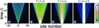
Fig. 1: (Color online) Time evolution of the density profile of fermions expanding in a lattice without observation, (a) for a single fermion; (b)-(d) for 13 fermions, initially located at adjacent lattice sites, calculated for several interaction strengths.

Stroboscopic many-body dynamics. We will focus on the expansion of an interacting cloud from an initially confined state. For 2-species fermions, such an expansion has been recently observed in 2D (Schneider et al., ) and theoretically discussed for 1D (Kajala et al., ). We will first briefly address the evaporation itself and then discuss qualitatively the resulting stroboscopic dynamics, with a more refined analysis presented further below. Figures 1(b)-(d) show the effect of the interaction on the unmeasured time evolution of the density profile. For increasing interaction the fermions tend to remain localized near their initial positions. For interaction strengths $|V/J|\apprge 3$ and the times shown here, $Jt<16$, a more detailed analysis reveals that evaporation proceeds via the rare event of a single fermion dissociating from the edge of the cloud. The particle then moves away ballistically. This evaporation process is hindered by the formation of bound states. This is a crucial phenomenon that we will also encounter in the context of repeated measurements. For smaller interaction strengths ($|V/J|\apprle 2$), the fermions split gradually into a larger and larger number of clusters as time increases. The parameter regimes in which the model (1) exhibits diffusive or ballistic transport was addressed using tDMRG in Ref. (Langer et al., 2009).

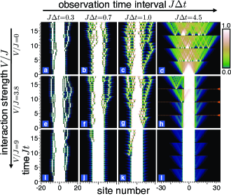
Fig. 2: (Color online) Specific realizations of the expansion of 13 fermions with site-resolved detection during the evolution. We show the full evolution of density even between observations, which collapse the many-body wave function at regular time intervals $J\Delta t$ [indicated by the dashed lines in panel (h)]. Without interaction [panels (a)-(d)], the initial decay rate of the configuration increases for larger $J\Delta t$, while for large interaction $|V/J|$ the decay rate is biggest for finite $J\Delta t$ [(g),(i)]. For small $J\Delta t$ the dynamics becomes independent of $\left|V/J\right|$, see (a),(e),(i).

The effects of stroboscopic observation are shown in Fig. 2, for typical realizations of this stochastic process. For noninteracting fermions we find the behavior expected from the single-particle case. The spread (and thus, the diffusion constant) increases with larger observation time intervals $J\Delta t$. For very small $J\Delta t$ (strong Zeno effect), the motion is diffusive with a small diffusion constant that becomes independent of $\left|V/J\right|$. In general, it is useful to discuss the initial decay rate of the cluster that evaporates via expansion. For the interacting case, this decay rate is largest at some finite observation time interval $J\Delta t$ [Figs. 2(g) and 2(i)], while it is reduced for large $J\Delta t$ [Figs. 2(h) and 2(l)]. Apparently, at very large $\left|V/J\right|$, the initial decay rate may have yet another local minimum for intermediate $J\Delta t$, see Fig. 2(j). We confirm this striking nonmonotonous behavior of the initial decay rate by simulating 400 realizations for each panel shown in Fig. 2 and plot the average number of fermions at the central 15 lattice sites as a function of time, in Fig. 3. For sufficiently large $\left|V/J\right|$, this number decays roughly linearly at a rate that sets the initial decay rate. We will see that these features can be mainly attributed to a bound state and the two-level dynamics between the initial state and the state with a fermion detached from the others.

Doublets and the role of interactions. The effect of interactions can be discussed already for the stroboscopic dynamics of two fermions. We focus on the decay of a doublet, i. e., two fermions sitting at neighboring sites.

In the quantum Zeno limit, $J\Delta t\ll$1 (or $J\Delta t\ll\left|2J/V\right|$ for large $\left|V\right|$, see below), only single hopping events occur during $\Delta t$. The probability for a fermion hopping left or right in this time interval is $2(J\Delta t)^{2}$. Thus, the average decay time of a doublet is $\langle Jt\rangle=1/(2J\Delta t)$, independent of $V$. This result holds also for clusters of more fermions, where the leftmost and rightmost fermion dissolves with probability $(J\Delta t)^{2}$ during $\Delta t$ [cf. Figs. 2(a), 2(e), and 2(i)].

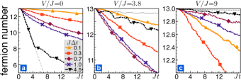
Fig. 3: (Color online) For the expansion process of Fig. 2, the average number of fermions remaining at the 15 central lattice sites is shown as function of the evolution time $Jt$ for different observation time intervals $J\Delta t$. Thin dotted lines correspond to expansions without observation. (a) Without interactions, the initial decay rate increases monotonically with $J\Delta t$. (b) At $V/J=3.8$, the decay rate first increases, then decreases with $J\Delta t$. (c) At $V/J=9$, the decay rate is nonmonotonous even for intermediate $J\Delta t$; compare $J\Delta t=0.3,0.7,1.0$. Note that the lines in (a)-(c) are almost identical for $J\Delta t=0.1$.

For larger $J\Delta t$, the interaction will become important, which gives rise to a bound state (this effect also exists for clusters of more particles (Sutherland, 2004)). Considering the basis $|l,K\rangle=\frac{1}{\sqrt{\mathcal{N}}}\sum_{j}\exp\{iK[j+l/2]\}c_{j}^{\dagger}c_{j+l}^{\dagger}|\textrm{vac}\rangle$ of the 2-particle sector with (positive) relative coordinate $l$, center-of-mass (c.m.) coordinate $j+l/2$, and total wavenumber $K=(k_{1}+k_{2})\,\textrm{mod}\,2\pi$, the action of the Hamiltonian (1) is $\hat{\mathcal{H}}|l,K\rangle=|K\rangle\otimes\hat{\mathcal{H}}_{K}|l\rangle$. The first part describes a plane wave with wavenumber $K$, the second the relative motion given by

$$\hat{\mathcal{H}}_{K}|l\rangle=-2J_{K}\big{[}|l+1\rangle+(1-\delta_{l,1})|l-1\rangle\big{]}+V\delta_{l,1}|l\rangle,$$ (2)

with $K$-dependent hopping amplitude $J_{K}=J\cos(K/2)$. A bound state exists if $|V|\geq|2J_{K}|$. It is given by $|\psi_{K}\rangle\propto\sum_{l=1}^{\infty}(-2J_{K}/V)^{l-1}|l\rangle$. We now discuss the decay of a doublet [see Fig. 4(a)] by means of the doublet survival probability $P_{D}(t)$, i.e., the probability of finding the doublet intact after time $t$. Without observations, $P_{D}(t)=\sum_{L^{\prime}}|\langle l=1,L^{\prime}|e^{-i\hat{\mathcal{H}}t}|l=1,L\rangle|^{2}$, where $L$ and $L^{\prime}$ are c.m. coordinates. Thus, in the limit $t\rightarrow\infty$, we find $P_{D}(\infty)=\frac{1}{2\pi}\int_{0}^{2\pi}\mathrm{d}K\left|\langle\psi_{K}|l=1\rangle\right|^{4}$. Specifically for large interaction $|V/2J|\geq 1$, we have

$$P_{D}(\infty)=1-\left(2J/V\right)^{2}+\frac{3}{8}\left(2J/V\right)^{4}\,.$$ (3)

While $P_{D}(\infty)$ is determined by the bound state, the evolution for times $Jt<1$ can be approximated by the two-level dynamics between $|l=1\rangle$ and $|l=2\rangle$. This gives

$$P_{D}(t)=1-\frac{1}{\pi}\int_{0}^{\pi}\mathrm{d}K\frac{\cos^{2}(K/2)}{\xi_{K}^{2}}\sin^{2}(2\xi_{K}Jt),$$ (4)

with $\xi_{K}=\left[(\frac{V}{4J})^{2}+\cos^{2}(K/2)\right]^{1/2}$.In the strongly interacting regime we find three regions for the doublet survival probability: for times $Jt\ll\xi_{K=0}^{-1}$ the probability is independent of the interaction strength, $P_{D}(t)=1-2(Jt)^{2}$; for times $\xi_{K=0}^{-1}\apprle Jt\apprle 1$ one expects an oscillating behavior of $P_{D}(t)$ given by Eq. (4) with a period approximately $\frac{2\pi}{V}$ for $|V/4J|\gg 1$; and for $Jt\gg 1$ the probability approaches $P_{D}(\infty)$.

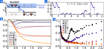
Fig. 4: (Color online) (a) Doublet decay level scheme. The doublet is separated from the continuum of unbound states by an energy gap $V$. (b) Probability $P_{D}$ of finding the doublet intact after evolution time $Jt$. Dashed horizontal lines show $P_{D}(\infty)$ found in Eq. (3). (c) Single trajectory of $P_{D}$ for a time evolution subject to observations. (d) Doublet survival probability $P_{D}$ as function of the observation time interval $J\Delta t\geq 0.02$ for a fixed total evolution time $Jt=18$. Note the non-monotonous dependence on $J\Delta t$ for finite interactions.

The full evolution of $P_{D}(t)$ using exact diagonalization is shown in Fig. 4(b). $P_{D}(t)$ is interaction-independent at times $Jt\apprle\xi_{K=0}^{-1}/2$. Temporal oscillations in $P_{D}(t)$ develop for higher interaction strengths ($V/J\apprge 3.5$). These oscillations suggest that in the presence of stroboscopic observations, illustrated in Fig. 4(c), the survival probability will depend nonmonotonically on the observation time interval. This effect is confirmed in Fig. 4(d). In that figure, the observation time interval $J\Delta t$ is varied, while keeping the total evolution time constant, $Jt=18$ (with a corresponding number of observations $t/\Delta t$). The stroboscopic evolution is interaction independent for small $J\Delta t$. For larger $J\Delta t$ there is a drastic recovery of $P_{D}$ in the strong interacting case, which can show oscillations as a function of $J\Delta t$. This behavior agrees with the one of clusters of more fermions, see Figs. 2 and 3, and does not depend in detail on the total time $Jt$. Thus we have found and explained the most prominent features of the stroboscopic many-body dynamics in our discussion of the doublet.

Furthermore, the motion of whole clusters of fermions through the lattice and the exchange of fermions between clusters can be observed in the stroboscopic dynamics, as shown in Fig. 5. As expected, clusters are very stable for high interaction strengths. The hopping amplitude for a cluster of $n$ fermions is of order $J^{n}/\left|V\right|^{n-1}$, decreasing strongly for larger clusters, as can be perceived in Fig. 5(c).

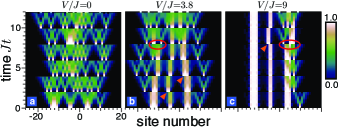
Fig. 5: (Color online) Density plot for the time evolution of an initial state with clusters of different numbers of fermions and observation time interval $J\Delta t=2$. For large interaction strength [panels (b) and (c)], we find clusters moving as a whole (indicated by triangles). Ovals indicate processes where single fermions are exchanged between clusters or attached to a new cluster.

Expectations for other models. The previously discussed nonmonotonic decay of a cluster is not unique for our model (1), but can also be observed in the Fermi-Hubbard (FH) and Bose-Hubbard (BH) models. In the following we will consider clusters of doubly occupied sites in 1D. The dissolution of a single particle from the edge of the cluster is well described by considering the survival probability of a doublon (fermionic or bosonic double occupancy). Using a similar analysis as for the doublets, one finds qualitatively the same behavior as shown in Fig. 4(b). However, this description is not sufficient to understand the decay of clusters. It does not include the escape of paired particles, which leads to a complete decay of the cluster in the long time limit even for large onsite interaction. It also neglects tunneling of bosons between occupied sites. In the FH model the cluster is initially Pauli blocked [as in model (1)], such that the dynamics is restricted to the edges. The escape of single fermions or doublons can be well approximated by the Hubbard dimer model, see (Kajala et al., ). The associated probability is $\sin^{2}(\sqrt{V^{2}+(4J)^{2}}t/2)/[2+2(J/4V)^{2}]$ for single fermions (at times $Jt\ll 1$) and for doublons it is $(Jt)^{4}$ for $Jt\ll J/V$ and $4(J^{2}t/V)^{2}$ at $J/V\ll Jt\ll 1$. We numerically verified that this oscillating behavior of the single fermion escape leads to nonmonotonic decay of the cluster for onsite interaction strengths $V/J\apprge 4$, see Fig. 6(a). The probability for an initial bosonic cluster configuration of $N$ sites to be destroyed is for short times given by $4[1+3(N-1)](Jt)^{2}$. The first term in brackets stems from a single boson escaping from the edge, while the second and larger contribution comes from a boson tunneling between occupied sites. For larger times we studied numerically the destruction of clusters [see Fig. 6(b)] and find that the survival probability of the initial cluster configuration displays a nonmonotonic behavior for $V/J\apprge 6$ with a pronounced local minimum at $t\approx\pi/V$ (about half the oscillation period for the dissolution of a boson and tunneling of a boson between doubly occupied sites), and the cluster is destroyed primarily via “internal” hopping processes. Both models show a strong nonmonotonic behavior of the cluster decay probability for large onsite interaction strengths. Thus, by tuning the time interval between observations in a stroboscopic measurement, one is able to enhance and suppress the decay of clusters, or even different decay channels of the cluster.

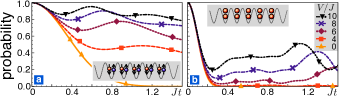
Fig. 6: (Color online) Destruction of a cluster in the 1D Fermi-Hubbard (a) and Bose-Hubbard model (b). We show the probability to detect a cluster of five doublons, see insets, in its initial state as a function of time for different onsite interaction strengths $V$.

Experimental realization and outlook. The Hamiltonian (1) is related to the Heisenberg $XXZ$ model by Wigner-Jordan transformation. The stroboscopic dynamics is identical for both models as the outcome of observations depends only on spatial density-density correlations. These Hamiltonians can be experimentally realized in optical lattices with fermionic polar molecules (Büchler et al., 2007) or 2-species fermions or bosons in the insulating phase (Duan et al., 2003; García-Ripoll and Cirac, 2003). For both realizations single-site detection has not yet been implemented, but experimental progress is being made toward this goal. Experimentally, the most challenging step needed to observe the interplay of many-body dynamics and measurements discussed here would be to make the observations nondestructive, whereas currently atoms are heated into higher site orbitals and atom pairs are lost due to light-induced collisions (Bakr et al., 2009; Sherson et al., 2010). Beyond the scenarios discussed here, one may also be interested in the influence of external driving or measurements that either are weak or target only specific sites.

Financial support by the DFG through NIM, SFB/TR 12, and the Emmy-Noether program is gratefully acknowledged.

Supplemental Material

Numerical implementation of the single-site resolved observation

An ideal single-site resolved observation of particles is a projective measurement in the basis of many-particle configurations (occupation number states in real space). However, due to the exponentially large number of states, we need a numerically efficient way to sample such outcomes. This is achieved by generating the measurement outcomes in a stepwise fashion, building on the fact that (positive) $n$-particle densities $\rho_{n}$ factorize into conditional probabilities

$$\rho_{n}(s_{1},\ldots,s_{n})=\rho_{1}(s_{1})\cdot\prod_{i=2}^{n}\rho_{i}(s_{i}|s_{i-1},\ldots,s_{1}).$$ (5)

Here, $s_{i}\in\{1,\ldots,N_{s}\}$ denotes the site of the $i$th particle and $\rho_{i}(s_{i}|s_{i-1},\ldots,s_{1})$ is the conditional probability of finding the $i$th particle at site $s_{i}$ given that there are $i-1$ particles at the sites $s_{1},\ldots,s_{i-1}$. The procedure starts by randomly drawing the position of the first particle from a distribution given by the one-particle density. In the next step, we draw the position of the second particle, conditioned on the location of the first one, and continue iteratively. This way less than $n\cdot N_{s}$ values of joint probability densities have to be calculated, in comparison to the full number ${N_{s}\choose n}$ of fermionic many-body configurations. This approach relies on being able to calculate efficiently both the pure time evolution between observations and the $i$-particle densities ($1\leq i\leq n$). In the present work, we use the time-dependent density-matrix renormalization group, which is an extremely powerful method for interacting one-dimensional systems. For the model considered in the main article, it is numerically even more efficient to draw the position of the first particle as before and then project the state onto those configurations where a particle is present at the selected site. After rescaling the resulting state, the new one-particle density is calculated. From this distribution we draw the position of the second fermion, excluding all sites already occupied by a fermion,and iterate the steps for the remaining fermions. For a discussion about local measurements on quantum many-body systems using matrix product states, see Gammelmark and Mølmer (2010).

Stroboscopic dynamics of noninteracting fermions

In the noninteracting case, we can explicitly calculate the $n$-particle densities needed to simulate the stroboscopic dynamics. After each observation, the many-particle wave function is a Slater determinant of single-particle wave functions, and for noninteracting fermions this remains true even during the subsequent time evolution. Using Wick’s theorem, the $n$-particle density of $N$ fermions at time $t$ can be written as (see also Löwdin (1955)):

$$\rho_{n}(s_{1},\ldots,s_{n};t)=\left|\begin{array}[]{ccc}M_{s_{1}s_{1}}(t)&\ldots&M_{s_{1}s_{n}}(t)\\ \ldots&&\ldots\\ M_{s_{n}s_{1}}(t)&\ldots&M_{s_{n}s_{n}}(t)\end{array}\right|.$$ (6)

Here, $M_{s_{k}s_{l}}(t)=\sum_{j=1}^{N}T_{s_{k}m_{j}}(t)T_{s_{l}m_{j}}^{*}(t)$, with the fermion propagator $T_{kl}(t)=i^{(k-l)}\mathcal{J}_{k-l}(2Jt)$, and the sum is taken over all initially occupied sites $m_{j}$. Note that the one-particle density $\rho_{1}(t)$ is just the sum of the densities of the individual fermions, cf. Fig.1(b) in the main article. Motion in arbitrary potentials would be captured by different propagators $T_{kl}(t)$.

References

- Bloch et al. (2008) I. Bloch, J. Dalibard, and W. Zwerger, Rev. Mod. Phys. 80, 885 (2008).
- Lewenstein et al. (2007) M. Lewenstein et al., Adv. Phys. 56, 243 (2007).
- Bakr et al. (2009) W. S. Bakr et al., Nature 462, 74 (2009).
- Sherson et al. (2010) J. F. Sherson et al., Nature 467, 68 (2010).
- Weitenberg et al. (2011) C. Weitenberg et al., Nature 471, 319 (2011).
- Misra and Sudarshan (1977) B. Misra and E. C. G. Sudarshan, J. Math. Phys. 18, 756 (1977).
- Itano et al. (1990) W. M. Itano et al., Phys. Rev. A 41, 2295 (1990).
- Fischer et al. (2001) M. C. Fischer, B. Gutiérrez-Medina, and M. G. Raizen, Phys. Rev. Lett. 87, 040402 (2001).
- Facchi and Pascazio (2008) P. Facchi and S. Pascazio, J. Phys. A 41, 493001 (2008), and references therein.
- Syassen et al. (2008) N. Syassen et al., Science 320, 1329 (2008).
- García-Ripoll et al. (2009) J. J. García-Ripoll et al., New J. Phys. 11, 013053 (2009).
- Daley et al. (2009) A. J. Daley et al., Phys. Rev. Lett. 102, 040402 (2009).
- Schützhold and Gnanapragasam (2010) R. Schützhold and G. Gnanapragasam, Phys. Rev. A 82, 022120 (2010).
- Shchesnovich and Konotop (2010) V. S. Shchesnovich and V. V. Konotop, Phys. Rev. A 81, 053611 (2010).
- (15) U. Schneider et al., arXiv:1005.3545v1 .
- (16) For Supplemental Material, see Appendix.
- Vidal (2004) G. Vidal, Phys. Rev. Lett. 93, 040502 (2004).
- Daley et al. (2004) A. J. Daley et al., J. Stat. Mech. (2004) P04005.
- White and Feiguin (2004) S. R. White and A. E. Feiguin, Phys. Rev. Lett. 93, 076401 (2004).
- Schmitteckert (2004) P. Schmitteckert, Phys. Rev. B 70, 121302(R) (2004).
- Pichler et al. (2010) H. Pichler, A. J. Daley, and P. Zoller, Phys. Rev. A 82, 063605 (2010).
- Barmettler and Kollath (2011) P. Barmettler and C. Kollath, Phys. Rev. A, 84, 041606(R) (2011).
- (23) J. Kajala, F. Massel, and P. Törmä, Phys. Rev. Lett. 106, 206401 (2011).
- Langer et al. (2009) S. Langer et al., Phys. Rev. B 79, 214409 (2009).
- Sutherland (2004) B. Sutherland, Beautiful Models (World Scientific, 2004).
- Büchler et al. (2007) H. P. Büchler, A. Micheli, and P. Zoller, Nature Physics 3, 726 (2007).
- Duan et al. (2003) L.-M. Duan, E. Demler, and M. D. Lukin, Phys. Rev. Lett. 91, 090402 (2003).
- García-Ripoll and Cirac (2003) J. J. García-Ripoll and J. I. Cirac, New J. Phys. 5, 76 (2003).

References

- Gammelmark and Mølmer (2010) S. Gammelmark and K. Mølmer, Phys. Rev. A, 81, 012120 (2010).
- Löwdin (1955) P.-O. Löwdin, Phys. Rev. 97, 1474 (1955).